Development of a reduced-order modeling technique for granular locomotion

(1)

Development of a reduced-order modeling technique

for granular locomotion

by

Shashank Agarwal

B.Tech., Indian Institute of Technology Gandhinagar (2014)

Submitted to the Department of Mechanical Engineering

in partial fulfillment of the requirements for the degree of

Master of Science in Mechanical Engineering

at the

MASSACHUSETTS INSTITUTE OF TECHNOLOGY

February 2019

@

Massachusetts Institute of Technology 2019. All rights reserved.

Signature redacted

Author...

Department of Mechanical Engineering

A!/ A /

Signature redacted

December 19, 2018

Certified by...

Accepted by...

MASSACHUSETTS INSTITUTE OF TECHNOLOGY

FEB

'2

5 2019

UiBiARIES

Kenneth Kamrin

Associate Professor

Thesis Supervisor

Signature redacted

Prof. Nicolas Hadjiconstantinou

Chair, Graduate Program Committee

(2)

(3)

Development of a reduced-order modeling technique for

granular locomotion

by

Shashank Agarwal

Submitted to the Department of Mechanical Engineering on December 19, 2018, in partial fulfillment of the

requirements for the degree of

Master of Science in Mechanical Engineering

Abstract

The work is aimed towards the development and expansion of a reduced-order mod-eling technique called granular Resistive Force Theory(RFT) for modmod-eling wheeled locomotion on granular beds. A combination of various modeling techniques, namely plasticity-based continuum modeling, discrete element method (DEM) modeling, along with RFT and collaborative experimentation are used for evaluation and ex-panding upon the capabilities of granular RFT. A dimensionless formulation cor-responding to the onset of catastrophic rise in slipping of wheels during granular locomotion is proposed. This limit also corresponds to the limits of the existing form of RFT in modeling wheel-granular media interaction accurately. Along with granular locomotion, general problems of granular intrusion have also been studied extensively using continuum modeling to characterize the general force response of different granular media based on various system parameters.

Thesis Supervisor: Kenneth Kamrin Title: Associate Professor

(4)

(5)

Acknowledgments

The completion of this work would not have been possible without the guidance and support of my research and academic advisor Prof Kenneth Kamrin. Ken has continually encouraged me to be a better student and researcher providing me with his invaluable tutoring and guiding me how to look into the details of simple yet challenging problems from a perspective of a researcher. I thank my parents and elder sister for their encouragement and constant support from overseas. Special thanks to our collaborator Andy Karsai and Prof Daniel Goldman at Georgia Institute of Technology whose expertise in experimentation has been vital for this work. I am thankful for all of my peers MechE, and the members of the Kamrin Group for making this entire experience a positive one. I am also indebted to an innumerable number of friends who have been there for me throughout my time at MIT. In particular, though, I want to thank Maytee Chantharayukhonthorn, my lab-mate and roommate, whose friendship I could not do without.

(6)

(7)

List of Figures

1-1 A real life example of sand flow . . . .

2-1 Evolution of wheel over time. . . . .

3-1 Schematic of Bekker's Bevameter intrusment . . . . 3-2 Stress field representation on rigid wheel as per TM model . . . . . 4-1 _{Comparison of RFT and Plasticity theory results in plate intrusion} 4-2 Fitted form of RFT force functions . . . . 4-3 Sample RFT simulations for various wheel shapes . . . .

5-1 Schematic of two particle interaction in DEM . . . .

5-2 Schematic representation of Non-cohesive graular model . . . .

14 15 22 23 27 29 31 34 35

6-1 Schematic and lab setup for force-slip experiments . . . . 40

6-2 Wheels nomenclature for slow locomotion study . . . . 42

6-3 A sample continuum simulation of wheel Type C . . . . 43

6-4 A sample RFT modeling of wheel type B . . . . 44

6-5 Wheel C on loose and compacted Poppy Seeds . . . . 47

6-6 Wheel A and B on compacted Poppy Seeds . . . . 50

6-7 Wheel C on MS and MMS . . . . 51

6-8 Comparison of RFT and TM model for wheel C on MS . . . . 54

6-9 Flapped wheel used in non-circular wheel locomotion study . . . . 57

6-10 Observations made in non-circular wheel locomotion studies . . . . . 59 7-1 7-2 7-3 8-1 8-2 8-3 8-4 8-5

Representation of system parameters associated with the flapped wheel Lab setup for flapped wheel experiments . . . . Normalized velocity variation with flapped wheel . . . .

Grousered wheel test setup for high-speed locomotion studies . . . . . Sample continuum simulation of grousered wheel . . . . High speed locomotion performance of grousered wheel: . . . .

Effect on initial velocity on equilibrium state for grousered wheels . . Variation of system parameters for different initial Velocity . . . .

62 63 64 66 67 69 70 71

(10)

8-6 Effect on the ramp rates on equilibrium state for grousered wheels . . 72

8-7 Dependence of critical angular velocity on various system parameters 74 9-1 Sokolovskii analytic form of Slip lines with characteristic log spiral . . 77

9-2 Continuum modeling: Flat plate intrusion in granular media . . . . . 78

9-3 Continuum modeling: Flat plate Intrusion in unconsolidated media 78 9-4 Continuum modeling: Intrusion of triangular intruder . . . . 79

9-5 Continuum modeling: Unsymmetric Triangle intrusion flow pattern 80 9-6 Continuum modeling: Unsymmetric Triangle intrusion . . . . 81

9-7 Force and flow transition in plowed granular media . . . . 82

9-8 Lift and drag forces in granular media . . . . 84

9-9 Lift and drag on cylinder: Variation of state variables . . . . 85

(11)

List of Tables

2.1 Evolution of wheel over time . . . . 16

4.1 Generic values of fitting parameters in analytic form of RFT . . . . . 28

6.1 Granular material properties for slow locomotion studies . . . . 41

6.2 Specifications of the wheels used in slow locomotion studies . . . . 42

6.3 Comparison of RFT, MPM and TM models for wheel C on CPS . . . 48

6.4 Comparison of RFT, MPM and TM models for wheel A and B on CPS 49 6.5 Comparison of RFT and MPM models for wheel C on MS and MMS 52 6.6 Comparison of RFT and TM model for wheel C on MS . . . . 55 8.1 Experimental and Simulation parameters for high-speed locomotion . 68

(12)

(13)

Chapter 1 Introduction: Granular media and its

triple nature

A granular material is a conglomeration of discrete solid, macroscopic particles

char-acterized by a loss of energy whenever the particles interact (the most common example would be friction when grains slide). Although granular materials are very simple to describe as the evolution of the particles follows Newton's equations, with repulsive forces between particles acting only when there is a contact between par-ticles, they exhibit a tremendous amount of complex behavior, much of which has not yet been satisfactorily explained. They behave differently than solids, liquids, and gases and yet quite similar to them in various scenarios which has led many to even characterize granular materials as a new form of matter. As an interesting fact, our world is full of granular materials, starting from naturally occurring substances like sand, snow, mud to food grains, which all fall under the category of granular media. In fact, the occurrence of granular media is not limited to naturally occurring substances and they actually constitute the second-most manipulated material (after water) in the industry. A huge variety of industrial and manmade materials fall un-der the category of granular materials including construction materials like cement and soil, pharmaceutical materials like medical pills and powders, food materials like grain, coffee beans etc.

The biggest hurdle and most the interesting challenge in modeling granular me-dia is their triple nature of promptly evolving between three state of matter: solid, liquid and gas in closely similar scenarios. For instance, in the Figure 1-1 a golf club hits the ground at high speed, while the person himself is standing on the sand itself where it acts like a solid, the stream of sand in front of him is similar to the flow of a stream of liquid, at the same time the sand can also be seen to be diffusing in air like a gas around the stream of sand. Such is the nature of sand which makes it extremely complex and difficult to model efficiently by a single unified method.

(14)

Figure 1-1: Flow of sand during a golf shot. [1]

This work primarily focuses the general problem of granular intrusion with the aim of developing a shape generic, reduced-order semi-empirical model for evaluation of resistive forces acting on various shaped rigid bodies intruding into various kinds of granular medias. Various kinds of preexisting modeling methods like plasticity-based continnum modeling and discrete element method (DEM) based modeling along with experimental validation is used with the ultimate aim of developing a quick, reliable and accurate method of modeling of general problem of granular intrusion. The work is primarily focussed on two related phenomena: 1) Wheel locomotion and 2) Rigid body intrusion into the granular media. While the field of wheel locomotion on sand (also called terramechanics in general) is chosen due to its large scale application as well as availability of large amount of pre-existing literature ( [2, 3, 4, 5]), the general problem of intrusion into sand was taken because it is fundamental to understanding all type of solid body-granular media interactions. The more details of the fields and our work is given in later chapters.

(15)

Chapter 2 Locomotion and wheels

2.1 History of development of wheels over time

Beside numerous fields of application mentioned in the previous chapter, one of the most important fields where the understanding of granular media is still restricted and needs more work is vehicular locomotion.

Locomotion is an important part of human existence. Humans made a huge leap in the field of locomotion as well as civilization itself upon invention of the wheel. Over the thousands of years, wheels have gone through a series of cycles of evolutions. The time line below [6] shows a high-level summary of important events which have taken place in the evolution of the wheel from its original form to current form.

Potter's Chariot Spoked Pneumatic Mordern

wheel wheel wheel wheel wheel

(16)

Table 2.1: Evolution of wheel over time 3500 BC 3200 BC 1000 BC 1802 AD 1845 AD 1888 AD 1910 AD 1911 AD 1926 AD 1954 AD Modern wheels

First use of wheel in Mesopotamia as potter's wheel First use of wheel in chariot in Mesopotamia

Invention of iron rim: starting of the use of wheels for transportation First wire tension spoke patented

First pneumatic wheel invented (Never commercialized:high cost) Pneumatic tire reinvented (Commercialized: Economic design) Carbon added to rubber to prolong tire life

Invention of tire-inner tube combination Inventions steel welded-spoke wheels Usage of tubeless tires started

Steel and alloy wheels: High performance (efficient and economical) Special wheels: extraterrestrial and military applications)

2.2 Differences of granular locomotion from rigid

surface locomotion

Even though the automobile industry has been a huge industry in itself for the past century, less work is done on the development of wheels meant specifically for gran-ular locomotion. An excerpt from the book 'the eyes of the desert rats' by David Syrrett [7] which talks about adventures of Brigadier Ralph A. Bagnold in Libyan deserts in the late 1930s gives an apt feel of what it feels like to travel on the sand with conventional tires:

... I increased speed to forty miles an hour, feeling like a small boy on a horse about to take his first big fence.... Suddenly the light doubled in strength as if more suns had been switched on. A huge glaring wall of yellow shot up high into the sky a yard in front of us. The lorry tipped violently backwards-and we rose as in a lift, smoothly without vibration. We floated up and up on a yellow cloud. All the accus-tomed car movements had ceased; only the speedometer told us we were still moving fast...

The paragraph is self-explanatory and says exactly what one observe when one tries to move over the sand (or any other granular media like dry snow for that matter). The place where locomotion of vehicles on any granular media vary from that on rigid roads is that while the performance of a vehicle on roads depends least on road itself (except in terms of energy losses in tires), the composite wheel performance while traveling on granular media is largely dictated by a relatively shallow, piece of ground that lies under the wheel and become directly involved in dynamic inter-play with vehicle's running gear (tires). The mechanical and deformation properties

(17)

of the driving media primarily define the complicit vehicle traveling behavior and hence the problem of vehicle locomotion expands from just vehicle dynamics to cou-pled vehicle and media dynamics. In the initial years of the 19th century during the development of automobiles, while the primary focus of tire development was on lo-comotion on rigid roads, people used their intuitions and experiences to develop ways of moving through sand. One such example is another excerpt from the same book

by David Syrrett

171

where Brig. Bagnold gives some strategies to drive over the sand:

... It should be taken at full speed on the high gear as far as possible, only

putting low gear when the speed slackens considerable and returning to high gear as soon as the sufficing acceleration has been obtained. Stopping anywhere on hard and slightly elevated ground should be avoided and getting into ruts of a preceding car is dangerous if the ground is sat all soft. A car will frequently go without difficulty in virgin ground but will stick if the same ground has been ploughed up by other cars...

While these strategies were extremely valuable in those days, they were more based on intuition and experience than mechanics based technical know-how. In the later years of the 1960s, interest towards locomotion over rough terrains (mainly sand deserts) increased especially with the work of Bekker

121

who gave a semi-empirical formulation for modeling rigid cylindrical wheel motion over the on non-cohesive sands. In the later years various authors

[8,

4, 9] expanded on the work of Bekker to develop various variations of Bekker theory for modeling wheel motion on different materials like drysnow [10], clay [11] etc. The most notable contribution to wheel-terrain modeling is the work by Wong and Reece which has become the de facto model of rigid cylindrical wheels on soft terrain [12, 13]. The model introduced

by Wong and Reece derives wheel torque, thrust, and sinkage by estimating the

stress distributions along the wheel-terrain contact region. The model is based upon the Bekker pressure-sinkage relation and the Janosi-Hanamoto shear-displacement equation [9]. A general formulation for modeling cylindrical wheel locomotion given

by Wong et al [12, 13] is explained in the next chapter.

2.3 Granular intrusion: A mechanics viewpoint

In this section, we carry out a general discussion about the various flow regimes a granular material encounters during a general intrusion process. A better under-standing of these regimes is vital for underunder-standing the dynamics of wheel locomotion because locomotion is essentially a large-scale non-linear intrusion process at the mi-croscopic level.

Dense, confined granular assemblies in quasistatic, slow shear flow are usually de-scribed as solids abiding by elastoplastic, rate-independent, constitutive laws [14].

(18)

Far from a confined granular state at large enough shear strains, where the material reaches the critical state, the material in a granular assembly is characterized by an internal friction coefficient y. In such a state the shear stress (T) in the medium is proportional to the normal stress (P), with a coefficient of proportionality [.

;T < pP (2.1)

= o'/v21 and P = (1/3)tr() (2.2)

where

o- _{is 3-dimensional stress tensor,}

t is the equivalent shear stress in the material,

P is hydrostatic pressure, and

y is called the internal coefficient of friction.

While in the quasi-static critical state regime the inertia of the grains is too small to be relevant, with increasing shear rates, various inertial effects start affecting the system. Major among them are discussed below:

2.3.1 Micro-Inertia

At low-pressure and/or large-shear rates, the inertia of grains starts affecting the effective strength of the medium [15]. This behavior is captured by a dimensionless number called the inertial number, I [161, which represents the ratio of inertial forces to confining forces. It has been found [17] that p is solely dependent upon

I for stiff particles at steady state. The various parameters in the collisional and

non-quasistatic regime obey:

T= P(I)P (2.3) p+(I) P 2 - Ps (2.4) I0/I+ 1 I = (2.5) 2P/ p8 where,

7 is equivalent shear stress in the material (given by equation 2.2),

P is hydrostatic pressure (given by equation 2.2), /u(I) is the internal coefficient of friction,

I , P2, andyit, are material constants,

y is shear strain rate,

d is the mean particle diameter, and Ps is the particle density.

It is important to note here that the above mentioned inertial effect is due to the inertia of individual grains relative to each other, which affects the coefficient of

(19)

friction of medium, and thus represents micro-inertial effects in the system. When the pressure, P , in the system is large and deformation rates are low, the medium is expected to be far from a collisional regime, and hence micro-inertial effects do not contribute significant variations in the effective coefficient of friction (p) of the medium.

2.3.2 Macro-Inertia

The macro-inertial effect associated with the bulk of grains affects the media's re-sponse when bulk velocity changes are high. A dimensionless macro-inertial number

-M, which is directly proportional to the inertia of the grains as a bulk and inversely

to hydrostatic pressure in the system: IM = (pv2_{)/P represents those effects in the}

system. The basic governing equations for nearly incompressible granular media in the rigid-plastic limit can be given as:

pi = -V.o-

+

pg (2.6)

a-=-PI + P(p, + Il )

i (2.7)

I0/I + I ID I

where

p is density of the medium, b is the material acceleration,

g is the acceleration due to gravity vector,

o- _{is 3-dimensional stress tensor,} P is hydrostatic pressure,

p, is static coefficient of friction,

Yd is upper coefficient of friction, I is a material constant,

I is the micro-inertial number, and

D is the strain-rate tensor, which is presumed to be roughly traceless during

dense flow where a constant-volume flow is expected.

Based on the formulation for IM provided above, it can be observed that that macro-inertial effects in the system are expected to be high only in regimes of high velocity or low pressure or both. The cases of high-speed intrusions correspond to such cases and hence dynamics of high-speed locomotion is more complex.

2.3.3 Elastic wave fluidization

The two effects described in previous sections do not account for any influence of grain stiffness. The particle stiffness, even if large, could also affect the strength of the medium during rapid impact if elastic waves through the medium cause contact

(20)

fluctuations. These fluctuations can increase fluidization as in [18, 191, and are of a different nature from the inertial effect of grain collisions described above. The effect could be quantified in terms of speed intrusion to speed of sound, V = /E/p, for elastic modulus, E. This effect is more likely to be observed at local flow velocities near V and not away from it.

(21)

Chapter 3 Traditional methods of modeling

wheel locomotion

3.1 Bekker's pressure-sinkage relation

As mentioned earlier, Bekker was among the very first authors who proposed a semi-empirical method of solving wheel locomotion whose underlying modeling approach relied on the analysis of two fundamental relations: the pressure-sinkage relation, and the shear stress-shear deformation relation. In the context of wheeled mobility, the pressure-sinkage relation governs the depth that a wheel will sink into the terrain when subjected to load, and consequently how much resistance it will encounter during driving. The shear stress-shear displacement relationship governs the amount of traction that a wheel will generate when driven, and therefore how easily it will progress through terrain and surmount obstacles. The pressure-sinkage relationship described by Bekker [2] was in the form of a semi-empirical equation that relates sinkage with the normal pressure of a plate pushed into the soil. The proposed relation is commonly referred to as the Bekker equation, and provides a link between the displacement (sinkage) and stress (pressure) of a plate (which can be viewed as a proxy for a wheel or track if one discretizes the leading surface of a wheel into sufficiently small sub-surfaces):

P= + k) zn (3.1)

Parameters kc, ko, n are empirical constants that are dependent on soil properties, while b corresponds to the plate width. These parameters can be obtained from field tests conducted with a device called a bevameter (Figure 3-1 [20, 5]).

(22)

LoeGng cybnders TOrSem Toem n t p pe e 3.2 M e dWmkX aBe Lker 9' press"r M gouge Pz e~ ~ PeersnPae

Figure 3-1: Schematic of Bevameter intrusment proposed by Bekker [2]

3.2 Modified Bekker model: Wong and Rees model

Over the past four decades, the original framework introduced by Bekker [2] has been expanded and modified by several researchers, and has found applications in many studies of wheeled and tracked vehicle's mobility [21, 22]. The most notable contribution to wheel-terrain modeling is the work by Wong and Reece which has, become the de facto model of rigid cylindrical wheels on soft terrain [12, 13]. The model introduced by Wong and Reece derives wheel torque, thrust, and sinkage

by estimating the stress distributions along the wheel-terrain contact region. The

model is based upon the Bekker pressure-sinkage relation and the Janosi-Hanamoto shear-displacement equation [9]. The details of the model are mentioned next.

The stress field under a wheel can be divided into two components (assuming a two-dimensional model, temporarily ignoring out of plane motion): normal stress and tangential stress. A schematic representation of the stress distribution at a wheel-terrain interface is presented in Figure 3-2.

Normal stress (-) can be calculated by beginning with Bekker's pressure-sinkage relation, then introducing a scaling function to satisfy the zero-stress boundary con-ditions present at the fore and aft points of contact of the wheel with the terrain (known as "soil entry" and "soil exit"). The equation is expressed as a piecewise

(23)

_r

-V

fi'~

r

J

hj*

Figure 3-2: (a)Normal and Tangential stress profile along a wheel surface and (b) Various associated parameters wrt. Wong and Rees Model

function, as:

or,1 = ( L, + k ) Z n 0 M < 0 < Of

92 = (k + ko ) Zn 0, < 0 < 0,

zi = r(cos 0 - cos Of)

Z2 = r cos (Of - Orn o (0, - O) - cos Of)

Om - or (3.2)

where Of is the soil entry angle, 0, is the exit angle, and 0m is the the maximum normal stress occurs. This angle can be calculated as:

Om

= (cI + c2 * s)Of

angle at which

(3.3)

where ci and c2 are experimentally obtained constant parameters defined in [8]. s

represents the slip and is defined as:

V V - V V

sw =t 1t - - - (3.4)

where, V is the actual forward speed of the wheel, Vt is the theoretical speed which can be determined from the angular speed w and the radius r of the wheel and V is the speed of slip of the wheel with reference to the ground.

The shear stress in the longitudinal direction is the primary source of driving traction. The shear stress T is a function of o-, soil parameters and the measured

shear displacement, J:

(3.5)

ME A

(24)

where c and

#

are the cohesion and the angle of internal shearing resistance of the terrain, respectively, and K is the shear displacement modulus which may be considered as a measure of the magnitude of the shear displacement required to develop the maximum shear stress (see [10]). J represents the shear displacement of the wheel edge with respect to the adjacent soil and is given as

/

Of dO

-Vtdt Vt (3.6)

0 0

where V is the tangential slip velocity given earlier in equation 3.4.

The thrust, T, is computed as the sum of all shear force components in the direction of forward wheel motion.

T br] Tcos OdO (3.7)

Compaction resistance, R,, is then computed as the result of all normal force components acting to resist forward motion.

RC = br -sin OdO (3.8)

Drawbar pull,F , is calculated as the net longitudinal force (i.e. the difference between the thrust force and resistance force). F, is the resultant force that can either accelerate the wheel or provide a pulling force at the vehicle axle.

F =T - Rc (3.9)

Driving torque can be obtained by integrating the shear stress along the wheel contact patch:

M = br2 _TdO _(3.10)

This set of equations constitutes the backbone of the model proposed by Wong and Reece, and it will be referred from here on as the TM model.

(25)

Chapter 4 Resistive Force Theory (RFT): A new

approach to model granular intrusion

4.1 Background

The traditional terramechanics approaches are formulated based on the understand-ing of the physical nature of vehicle-terrain interaction, and detailed analyses of the mechanics of wheel-terrain interaction. These models rely on a set of parameters that include intrinsic soil properties such as cohesion and internal angle of friction, along with semi-empirical parameters including the shear modulus and the sinkage coefficients and hence are often over-parametrized and require adhoc terrain testing. Hence the usage of these modes for modeling wheel locomotion typically results in limited performance when wheel geometry is modified, when operational conditions diverge from nominal conditions (e.g., the high slip condition), and when parame-ter estimation from wheel performance data is attempted. On the other hand, ap-proaches based on RFT have the advantage of relying on a compact set of parameters and can be applied to a wide range of wheel geometries. While the traditional ter-ramechanics approaches by various authors like Bekker [2], Janosi and Hanamoto

[9J,

Wong and Reece [121 etc are based on detailed understanding of the physical nature and mechanics of wheel-terrain interaction, major caveats of all of them includes their specialization for locomotor shapes (In most of the cases cylindrical rigid wheel geometries assuming plane-strain deformation in sand) and dependence on various intrinsic material properties (like cohesion and internal angle of friction in wong model) and 'semi-empirical' parametric properties which are specialized for specific wheel geometries (like angle of maximum normal pressure, fore and aft angles etc in wong model). While having specificity to shapes limits applicability of these models to 'modified' wheel shapes in various situations, over parameterization like 10

pa-rameters in case of Wong and Reece model (namely K, , K0 , n , ao, ai,#, c, kx,6 e,

(26)

re-calibrations require large numbers of experiments to be performed using some specialized experimental setups like the Bevameter in Bekker model. For countering all these caveats, the main focus of our research, granular Resistive Force Theory, comes at rescue due to its compact closed loop formulation. More details of the method are mentioned in the next section.

4.2 Resistive Force Theory based locomotion

RFT was originally a theory introduced in the literature of fluid mechanics used to approximate Stokesian behavior in order to model undulatory and flagellar propul-sion in viscous fluids at low Reynolds numbers [23]. For an object which locomotes

by swimming through fluids (such that the velocity on each part of the swimmer

takes different values), while finding an analytical expression of the total drag forces is difficult (from the Navier-Stokes equations) using Numerical computation is ex-pensive. Hence, Gray and Hancock [23] approximated a solution to such problems by postulating that the force field on an infinitesimal element of a slender body (whose radius of curvature is significantly larger than the width) is hydro-dynamically de-coupled from the rest of its body. Thus the drag force on an element (of very simple geometry) can be computed from its tangent direction

i

(or normal ft) and local velocity. Once the force on each individual element is known, the net drag for the swimmer is given by a linear superposition.

Following on the same lines, granular RFT was recently adapted by Maladen et al [24] to solve the problems of subsurface swimming in granular media. Unlike viscous fluids, for an intruder moving slowly in granular materials, the drag force is dominated by friction: it is independent of the moving speed and increases with penetration depth. The RFT formula then takes the form:

Fd =

J

kpzI[fl,(V- -t)i +

f(v

-

n)i]ds,

(4.1)

where kpgz| is the local overburden pressure on a small element ds of the intruder at the depth IzI. When granular RFT was first developed, the functional forms of

f'

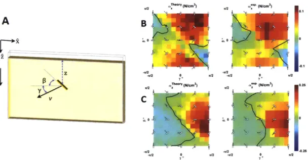
and fii were determined from experimental trials [24, 25].

To make the formulation more structured, components fi and fil are refined in form of a, and oz which represents force per unit area per unit depth in x and z directions in the lab reference frame (gravity in the positive z-direction). More details about the integral form of RFT are discussed in the next section. Though the initial force function of RFT (in form of a,,) were proposed using experiments, Askari and Kamrin [26] later successfully verified that the functional form obtained using experiments earlier can also be derived using conventional Mohr-Coulomb plasticity (shown in figure 4-1, giving an indication of possible explanation of origins of RFT.

(27)

.1W2 C -.12 -W12 0 1 x/2 a(ICM 3) 0.21 - SC W2 .7 C) 2

Figure 4-1: (A)Illustration of RFT associated parameters on a small plate intrusion geometry. (B,C) Results of plasticity theory simulation vs. experimental measure-ment of resistive forces in granular media using a small plate elemeasure-ment, showing the horizontal (a, ) and vertical (a, ) stresses per unit depth in a bed of glass beads.

It is also interesting to note here that though granular RFT has its inspiration from its fluid counterpart, granular RFT has demonstrated to be more effective in modeling the forces in granular interactions with intruders than its viscous coun-terpart in locomotion in the quasistatic locomotor regime, and jumping on granular media (27, 28].

4.3 Using RFT for force calculations

We now explain the basic strategy used in the calculation of forces acting on an arbi-trarily shaped body using RFT formulation presented by Li et al [25]. As mentioned above the basic philosophy of RFT is decoupling of forces on various sub-surfaces of the body and using linear superposition to calculate the net forces. Hence, for a convex-shaped solid slowly intruding into granular material, one can decompose its intruding surface into arbitrarily small leading surfaces. Then, the force for each sub-surface is calculated as a function of the intruder's orientation angle / and the intrusion velocity vector angle -y (refer to Figure 4-1(A)). By simply summing over the forces experienced by the small leading surfaces, the net resistive force on the whole intruder is calculated. In two dimensions, the resistive force(f ,

f,)

on an intruder can be calculated as:

A

9g

(28)

(fx, fZ) = ((Ox ( , -y), a ,(0, -y)) H(z) Iz Ids (4.2)

where H(z) is the Heaviside function whose value goes to 1 only when a surface is submerged in ground else its zero and z is the intrusion depth from the surface of the ground and is always positive. The stresses upon these intruding surfaces are defined by the functions ax,, which represent force per unit area per unit depth. RFT takes an empirical approach by determining these functions through repeated slow experimental intrusions of a small flat plate submerged a unit depth in the tested media at various values of / and -y (figure 4-1(A)), creating a force diagram from force measurements for these angled surface elements (figure 4-1(B,C)). These small elements obey linear superposition and can be applied to any desired intrusion surface. Thus this simple closed form equation makes granular RFT a useful tool for estimating the forces on both submerged and intruding bodies in granular media. While the original dependence of ax,, was obtained in form of experimental data, Li et al [25] derived a trigonometrical form of generic values of the same as a function of

3

and -y by performing a Fourier analysis on the graph shown in figure 4-1(B,C). Before performing the analysis, axz were converted into two components owing to the fact that general form of force response for most of the non-cohesive materials is same, differing only by a constant factor among themselves. The components consist of a grain-structure interaction parameter, , and the generic values of age. Force function splitting for ax,z, functional forms for agez and corresponding fitting graphs are shown below:

aX,= * gen (4.3)

~en 1 m# ny m# n+ y

age" = [Am,ncos2( + ) + Bm,nsin2r( + )] (4.4)

m=-1 n=O

1 1

genm n-y i (m# n-y (45

CXen = [C,ncos27( + -) + D,nsir2r( + )] (4.5)

m=-1 n=O

In the above formulation, considering terms whose magnitudes are greater than

0.05 A0,0, only following 9 terms were found to be significant (With the value of each

component mentioned in the table)

Table 4.1: Generic values of fitting parameters in analytic form of RFT Parameter A₀,₀ A₁,₀ B₁,₁ Bo,₁ B ₁,₁ C1,1 C0,1 C_1,1 D1,o

Values 0.206 0.169 0.212 0.358 0.055 -0.124 0.253 0.007 0.088

It is important to note here that though RFT has a more compact form, terrame-chanics models can be utilized for broader terrain types (granted proper

(29)

characteri-a generic (Ncm3) 0 0

fz

B

1n/2 0*0

I

~1 n/2 Z

Figure 4-2: Fitted form et al [251 formulation

of RFT force functions obtained using Forier analysis by Li

zation) and velocity regimes where the applicability of granular RFT (especially to cohesive soils) is yet to be verified.

4.4 Modeling wheel locomotion using implicit RFT

code

Following on the lines of the RFT formulation mentioned in the previous section, the following section explains the core functioning of an iterative implicit RFT scheme implemented in MATLAB®. In terms of material/system properties, a single scaling parameter() is required which is sufficient to characterize complete wheel-terrain interaction properties. The formulation is applicable for any wheel shape and some examples are shown at the end of the section.

The overall system consists of two parts, an intruding body, and the media being intruded. To begin with, utilizing the rigid wheel assumption, the wheel surface is discretized into smaller sub-surfaces that together approximated the total geometry of the wheel. The orientation, velocity direction, depth, and area of each sub-surface along with normalized force per unit depth (oz") from Li et al [25] and associated scaling coefficients ( ) is used for finding the resistive forces from the media on each subsurface. The net resistive force and moment on the wheel are then calculated

by using a linear superposition principle mentioned previously along all the leading

surfaces of the body as shown representatively in equations below. In performing all these simulations, a 'leading edge hypothesis' was used which made sure that

A

n/2 (N/cm 0I.4 120.4 ,t/2 Ck 0 -1

(30)

the resistive forces experienced by the wheel consisted contributions from only those surfaces which were moving 'into' the sand (and not other way round as the other case would have represented the cohesive nature of sand). That is,

Fresistive =

f

((ax(, -y), a.(, y))H(z)IzIds (4.6)

ax,( P, ) = a ((, Y) (4.7)

where,

FResistive is the total resistive force acting on the wheel (intruding body),

az,x are material specific force functions [Stress/depth], Z," are universal generic force functions [Stress/depth],

( is the grain-structure interaction parameter (Scaling parameter),

#

is angles of inclination [Fig 4-11,

y is angles of intrusion velocity [Fig 4-11,

H(z) is the heaviside function ( = 1 if surface is submerged, 0 otherwise), z is the intrusion depth and is always positive,

Once the net resistive force is known, the wheel's motion is then captured using a momentum balance in the x-z lab frame coordinates

M'bcm =F gravity + FResistive + Fexternal (4.8)

where, M is the mass of the wheel,vcm is the velocity of the wheel's center of mass,

Fgravity is the force vector on the wheel due to gravity and FExternal is the external

force vector on the wheel (e.g. pulling forces etc).

It is to be noted that a special kind of forced slip experiments were also simulated using the RFT implementation (Chapter 6). In such cases, the wheel's translation, as well as angular velocities were predefined. Hence for such cases, a momentum balance in the x lab frame coordinate and angular momentum balance along the axis of the wheel, gave the values of total drawbar pull and torque (respectively) which wheel required to sustain the given velocity conditions. The vertical motion (Sinkage) of the wheel was captured by doing a momentum balance in z lab frame coordinate.

(31)

Red: Velocities Blue: Forces Z Granular Media Red: Velocities e: Forces Granular Media Red: Velocities Blue: Forces x Granular Media Red: Velocities Blue: Forces x Granular Media

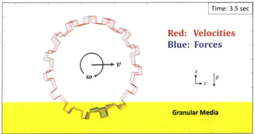
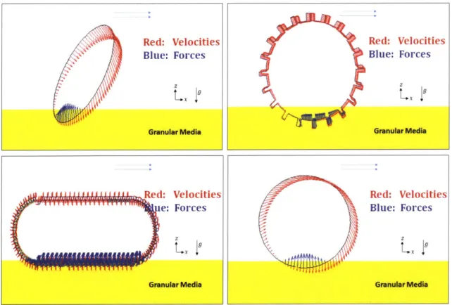
Figure 4-3: Simulations of various wheel shapes A) Elliptic wheel, B) Grousered wheel, C) Tank treads and D)Cylindrical wheel) using implicit RFT code

(32)

(33)

Chapter 5 Computationally intensive methods

of simulating granular media

5.1 Background

The two semi-empirical approaches mentioned so far, namely terramechanical as well as RFT, have the advantage of being extremely efficient in the terms of computational effort required. But the low computational cost in both the methods comes at the expense of lesser information about the system. Both the methods provide with the stress at the surface of the wheel and do not provide any information about the media in which intrusion itself is taking place. The scenario is not undesirable as the objective of the methods was to evaluate the forces only but for expanding upon their fields and scenarios of applications of both the methods, a full system modeling is required. We use two different methods for full system modeling:

" Discrete element Method based Molecular Dynamics (MD) modeling " Material Point Method(MPM) based Continuum modeling

5.2 Discrete Element Method (DEM

I

MD)

Discrete Element method is a well-established method of particle modeling which takes into account each particle of the system for modeling the system. We use Molecular Dynamics (MD) based LAMMPS software from modeling grains as and when required. The basic details of particle modeling are given further. The model being used in our work uses an inbuilt granular model based on work on Brinliantov and others [29, 30, 31]. The methods involve solving various system parameters at the individual particle level, taking into account the normal and tangential forces acting on adjacent, interacting particles, numerically integrated to find positions and

(34)

velocities. The model uses Hookean contacts for force calculation between a pair of particles and velocity verlet algorithm for position and velocity update (second-order accurate in time).

A B

R

Figure 5-1: (A)Schematic of two particle interaction [29], (B) A sample 2D plane-strain plate intrusion simulation using LAMMPS

For the calculation of forces following formulation is utilized:

F = (knij - meff nvn) - (ktAst + meff ytvt) (5.1)

Ft < pF, (5.2)

The first equation above is Hookean contact definition. Force in normal direction is directly proportional to overlapping distance 6n1 and force in tangential direction is

proportional to history-dependent tangential overlap Asj. The force also contains the effect of damping in the normal and tangential direction in form of N2 and 'yt

co-efficients. The second equation is the coulomb friction condition. While this method can be highly precise, large scale differences between the size of the simulated system and the individual particle size make the number of individual particles involved to be very large. For example, a 10cm x 10cm x 10cm system of particles of size 0.5mm would have 8x106 particles and 48x106 variables to solve (3 positions and 3 veloc-ities) for each time step. Despite its computational cost, DEM remains the most reliable and proven technique at hand for modeling complex granular interactions. We primarily use this method for performing 2 and 3-dimensional intrusion scenarios at different velocities. Figure 5-2 shows a sample 2D flat plate intrusion experiment done using LAMMPS. Quantitative results are shown in relevant sections.

(35)

AJ

5.3 Continuum modeling

5.3.1 Constitutive laws

While DEM methods are highly accurate but are computationally expensive, mean-while, a continuum model based computation can solve the same system by consid-ering carefully selected chunks of material as blocks of uniform state to save large amounts of computation time. As mentioned earlier, the work of Askari and Karmin

[26], in being successful to be able to regenerate current form of RFT was

indica-tive of the fact that continuum modeling is a reliable tool of modeling low-velocity granular locomotion. A quick overview of the method and implementation is given later in this chapter. For more details, their paper can be referred [26]. Motivated

by their work we implement following three constitutive models using 2D Material

Point Method code developed by Dunatunga et al [32].

" Non-cohesive Granular media model

* Critical State Model for granular media Non Cohesive Granular media model

This model was included in the original work of Dunatunga et al [32]. The main properties of granular media being captured by the model are two: 1) Shear strength of the material is proportional to Hydrostatic Pressure (only for positive pressure). 2) The material loses all its strength if the density of the medium goes below the critical density. The free expansion prevents the system from ever having tension. Given below is the mathematical form of the model. Note that this sand model was obtained from p(I) by assuming I ~ 0 and that grains separate into a stress-free medium when below a critical density:

P

Figure 5-2: Schematic representation of Non-cohesive graular model. (Left) shear strength of material depends on Pressure. (Right) Material can not support tension.

(36)

P = 0 if P < Pc (5.4)

= 0 if P=O (5.5)

where,

= o'/v 21 Equivalent shear stress,

P -1/3(tr(o)) Hydrostatic Pressure,

ao = 0 + P1 Deviatoric part of stress tensor AND pc is the critical density of the material.

Linear Critical State Model for granular media

This model is an improved version of the previous non-cohesive sand model because this model allows for density variation in media [331. As an important observation, it can be observed from the constitutive equations that the gradient of packing fraction

(#) over time always tries to evolve system towards the critical state density (in case

of deforming media):

Ac = Ps + (0 - #ss)X (5.6)

do=

(# - #")#x3 _(5.7)

dt

where,

0sC" is Steady state critical packing fraction

p," is Coefficient of Internal friction at steady state critical packing fraction

x Dimensionless scaling constant i Equivalent shear strain rate

For the purpose of implementation, the packing fraction was converted into the ratio of local medium density and grain density

= P/Pgrain (5.8)

Using the above substitution, the evolution equation for

4

gives:

1

-dp ( C S)#oi (5.9)

Pgrain dt

dp _dt _(5.10)

(p - Osjpgrain)p Pgrain

Using Pn = m/vn for a material point, where Vn is volume and m is mass of material point at time step n. And integrating both sides from tn to tn1

ln(1 - Sc Pgrainv V" i - (5.11)

m

V

(37)

Implicit volume update at each step is found as:

/3(

m Vne = 3vn + (1 -

)

(5.12) Pgrain&bs where, 13 = exp(-Xy#O"At)

This volume update (along with the density value below which material losses all its strength) is the only additional update in the previous non-cohesive model whose details can be seen in Dunatunga et al

[32].

5.3.2 Implementation

Attempts are being made by various authors including Dunatunga and Kamrin

[32]

to use the Material Point Method (MPM), a derivative of the fluid-implicit-particle (FLIP) method [341, based on the particle-in-cell (PIC) method [35] to perform granular plasticity simulations. The key idea behind MPM is that the state of the simulation is contained in Lagrangian material points, while the equations of motion are solved on a background computational mesh in a manner similar to FEM. Since the state is saved at each material point, the mesh is reset at the beginning of each computational step allowing for large deformations without mesh distortion. The basic computational layout for granular media is extensively discussed in Sulsky et al. [36]. Successful implementation, along with experimental verification of MPM, was done by Dunatunga et al for scenarios in high-speed intrusions. The model being developed by them for dry non-cohesive sand could be used in simulating locomotion and intrusion scenarios in various granular media and has been utilized here. For the implementation of various different intrusion scenarios (geometry and motion), evaluating and updating specific system properties and implementation of new material models, the materials files are updated as and when required.

(38)

(39)

Chapter 6 Low speed Locomotion

6.1 Circular wheel locomotion

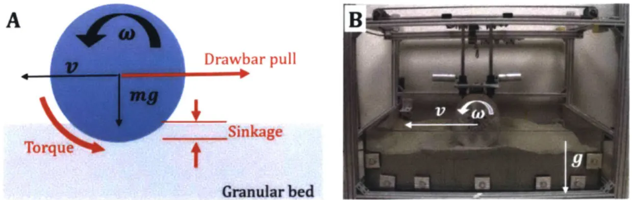
With all the methodologies discussed in the previous chapters, we start with the problem of modeling a plane strain cylindrical wheel motion on a test-bed of non-cohesive granular material moving under low-velocity forced-slip conditions. While low-velocity locomotion represents the velocity regime in which the sand under the wheel can be considered to be in quasi-static state (more discussion about how to decide and define 'low velocity' limits, is done in next chapter on high-velocity speed locomotion), the forced-slip condition means that the wheel moves at a fixed prede-fined sets of angular velocity (w)and transnational velocity(v) conditions throughout the run. The output parameters being studied were drawbar force (required to be applied on the wheel to maintain input translation velocity), torque (required to be applied to maintain input angular velocity) and sinkage (resulted as a function of the constrained motion of the wheel). Figure 6-1 shows an equivalent system schematic as well as actual experimental setup being used for the study. A brief summary of the experimental setup and input parameters is given in the next section.

6.1.1 Experimental details

The data collection for experiments was done by a previous student in collaboration with Crab Lab at GeorgiaTech, Atlanta. Hence limited details about the data col-lection are given in this document but more details about the same can be obtained in the relevant paper.

Testing Rig

The 1m long, 0.6m wide and 16cm deep Lexan Testbed shown in Figure 6-1 B. A carriage slides on two low-friction rails attached to the main aluminum frame allows

(40)

A

B

Drawbar pull

Sinkage Torque

Granular bed

Figure 6-1: A) Schematic and B) Experimental setup of forced-slip Terramechanics rig used in the study, where translation (v) and angular velocities (w) are controlled while Torque, Drawbar pull and Sinkage (z-direction motion is free) are measured

for controlling longitudinal translation of the wheel. The wheel mount was allowed to freely translate in the vertical direction. Thus the translational and the angular velocity of the wheel as well as applied vertical load were controlled. As mentioned earlier, the experiments were conducted under a forced slip condition, the wheel angular velocity w and wheel longitudinal velocity v were controlled according to:

slip = 1 - V (6.1)

rw where

slip is the desired slip ratio and r is the nominal wheel radius.

In the experiments wheel-angular-velocity was held constant while longitudinal ve-locity was varied to achieve the desired slip ratio. In terms of output parameters, draw-wire encoders were used for horizontal and vertical displacements, a 6-axis force torque transducer mounted between the wheel mount and the carriage was used to measure the vertical load and traction generated by the wheel and an ange-to-ange reaction torque sensor was used to measure the driving torque applied to the wheel. The rig was capable of providing approx 1m run, 120 mm/s maximum translation velocity, and 400/s of wheel angular velocity. For the experiments with Poppy Seeds, a similar setup with controlled packing fraction was used. The vertical loads were varied between 18 N and 190 N mentioned in related experiments.

Materials

Three simulants were used in this work: Quikrete 1962 medium sand (MS, predom-inantly silica particles of size 0.3-0.8mm), Mars Mojave Simulant (MMS, mixture of

(41)

finely crushed and sorted granular basalt with 80% of particles within 10,pm intended to mimic, Mars soil characteristics) and Poppy Seeds (PS). Various soil properties measured using standard plate penetration tests and terra-mechanical methods [10 are presented in Table 6.1. Specifically, MS and MMS were characterized through plate penetration tests and direct shear tests. The RFT constant for these simulants was extrapolated from the plate penetration tests. The Poppy Seeds (PS) on the other hand, were only characterized by plate intrusion experiments.

Table 6.1: Granular material properties for slow locomotion studies

MS MMS PS (# = 0.58) PS (# = 0.60)

k, [kN/mn+1J -2.05e+4 846 -2.06e+5 -3.24e+5 k. [kN/mn+2] 3.13e+6 6708 7.07e+6 1.11e+7

n 1.0 1.4 1 1 c [Pa] 1500 600 0 0 4D [deg] 34 35 36 45 kx [m] 0.0006 0.0006 0.045 0.045 RFT Constant [N/cm 3l 2.02 3.05 0.35 0.55 K [m] 0.0006 0.0006 0.045 0.045 Pgrain [kg/M3] 2600 2875 1100 1100 Packing Fraction

#

0.6 0.6 0.580 0.605 MPM : Pinternal 0.53 0.50 0.53 0.54 MPM : Psurface C: 0.55 C: 0.55 C: 0.55 C: 0.55 B: 0.35 B: 0.35 A: 0.60 A: 0.60

For the MPM based continuum modeling, it was assumed that the motion of

all the wheels considered in this study can be modeled as plane strain problems (which is a justifiable assumption to take if the out-of-plane depth of contact area between wheel and sand is larger than its width). The plastic flow parameters for the simulations were calibrated by matching zero-slip experimental data to zero-slip

plane-strain MPM simulations. Since the actual deformation in experiments was

not always strain, we accept potential inaccuracy brought about by the plane-strain simplifying assumption.

The MPM simulations were found to be most sensitive to the internal coefficient of friction of sand (MS/MMS/PS). The effective internal friction values (plinternal) for each media was evaluated by finding the value of Pinternal which when used in MPM simulation results in the same sinkage as found experimentally. This matching was done once (for the zero-slip case) for each media and once that value was obtained, the same value was used for all the simulations throughout the study. Values for all four materials are shown in Table 6.1. Calibration trials for deciding the surface friction

(42)

coefficient (Psurf ace) between the wheels and the sand were found to be accurate

enough with the use of original 3D friction coefficients and hence various original wheel-sand pair values (reported in Table: 6.1) were used.

Wheels

Experiments were conducted with width/radius) of 0.5, 1.05 and 1.23. dimensions are given in Table 6.2. while wheel C has been tested also

three different wheels with aspect ratios (i.e., The wheels are shown in Figure 6-2, while wheel Wheels A, B, and C have been tested on PS, on MS and MMS.

Figure 6-2: Wheels nomenclature for slow locomotion study (Image not to scale).

Table 6.2: Specifications of the wheels utilized in this study experiment conducted. Surface coating, 60 grit, PLA, MMS.

and summary of the

A B C

Type Smooth Wheel Lugged Wheel Smooth Wheel

Radius [mm] 101.6 72.5 (to lug tips) 130

Aspect Ratio 0.5 1.05 1.23

PS V V

MS -

/

MMS -

/

Vertical Loads [N] 20 18 80-190

Wheel A is a Nylon wheel with a narrow aspect ratio. The wheel surface was coated with 60 grit sandpaper in order to guarantee sufficient friction at the wheel-terrain interface. Wheel B was manufactured using a MakerBot Replicator II 3D printer using PLA filament. The wheel has 15 lugs, equally spaced, 10 mm tall and

11 mm thick, which span the whole width of the wheel. This wheel has no sandpaper

coating, as the presence of the lugs guarantees sufficient wheel-terrain engagement. Finally, wheel C is an aluminum cylinder coated with MMS. For continuum modeling of wheel-media surface interaction, the coefficient of surface friction for wheel C with

Development of a reduced-order modeling technique for granular locomotion

Development of a reduced-order modeling technique

for granular locomotion

by

Shashank Agarwal

B.Tech., Indian Institute of Technology Gandhinagar (2014)

Submitted to the Department of Mechanical Engineering

in partial fulfillment of the requirements for the degree of

Master of Science in Mechanical Engineering

at the

MASSACHUSETTS INSTITUTE OF TECHNOLOGY

February 2019

@

Massachusetts Institute of Technology 2019. All rights reserved.

Signature redacted

Author...

Department of Mechanical Engineering

Signature redacted

December 19, 2018

Certified by...

Accepted by...

FEB

'2

5 2019

UiBiARIES

Kenneth Kamrin

Associate Professor

Thesis Supervisor

Signature redacted

Prof. Nicolas Hadjiconstantinou

Chair, Graduate Program Committee

Development of a reduced-order modeling technique for

granular locomotion

by

Shashank Agarwal

Abstract

Acknowledgments

Contents

List of Figures

List of Tables

Chapter 1

Introduction: Granular media and its

triple nature

Chapter 2

Locomotion and wheels

2.1

History of development of wheels over time

2.2

Differences of granular locomotion from rigid

surface locomotion

171

121

[8,

2.3

Granular intrusion: A mechanics viewpoint

2.3.1

Micro-Inertia

2.3.2

Macro-Inertia

+

2.3.3

Elastic wave fluidization

Chapter 3

Traditional methods of modeling

wheel locomotion

3.1

Bekker's pressure-sinkage relation

3.2

Modified Bekker model: Wong and Rees model

fi'~

r

J

Om

#

/

Chapter 4

Resistive Force Theory (RFT): A new

approach to model granular intrusion

4.1

Background