Forecasting temperature in a smart home with segmented linear regression

(1)

Publisher’s version / Version de l'éditeur:

Vous avez des questions? Nous pouvons vous aider. Pour communiquer directement avec un auteur, consultez la première page de la revue dans laquelle son article a été publié afin de trouver ses coordonnées. Si vous n’arrivez pas à les repérer, communiquez avec nous à PublicationsArchive-ArchivesPublications@nrc-cnrc.gc.ca.

Questions? Contact the NRC Publications Archive team at

PublicationsArchive-ArchivesPublications@nrc-cnrc.gc.ca. If you wish to email the authors directly, please see the first page of the publication for their contact information.

https://publications-cnrc.canada.ca/fra/droits

L’accès à ce site Web et l’utilisation de son contenu sont assujettis aux conditions présentées dans le site

LISEZ CES CONDITIONS ATTENTIVEMENT AVANT D’UTILISER CE SITE WEB.

Procedia Computer Science, 155, pp. 511-518, 2019-09-13

READ THESE TERMS AND CONDITIONS CAREFULLY BEFORE USING THIS WEBSITE. https://nrc-publications.canada.ca/eng/copyright

NRC Publications Archive Record / Notice des Archives des publications du CNRC :

https://nrc-publications.canada.ca/eng/view/object/?id=a75586a5-3883-4335-b1a9-64dfe606af09

https://publications-cnrc.canada.ca/fra/voir/objet/?id=a75586a5-3883-4335-b1a9-64dfe606af09

NRC Publications Archive

Archives des publications du CNRC

This publication could be one of several versions: author’s original, accepted manuscript or the publisher’s version. / La version de cette publication peut être l’une des suivantes : la version prépublication de l’auteur, la version acceptée du manuscrit ou la version de l’éditeur.

For the publisher’s version, please access the DOI link below./ Pour consulter la version de l’éditeur, utilisez le lien DOI ci-dessous.

https://doi.org/10.1016/j.procs.2019.08.071

Access and use of this website and the material on it are subject to the Terms and Conditions set forth at

Forecasting temperature in a smart home with segmented linear

regression

(2)

ScienceDirect

Available online at www.sciencedirect.com

Procedia Computer Science 155 (2019) 511–518

This is an open access article under the CC BY-NC-ND license (http://creativecommons.org/licenses/by-nc-nd/4.0/) Peer-review under responsibility of the Conference Program Chairs.

10.1016/j.procs.2019.08.071

10.1016/j.procs.2019.08.071 1877-0509

www.elsevier.com/locate/procedia

The 9th International Conference on Sustainable Energy Information Technology (SEIT)

August 19-21, 2019, Halifax, Canada

Forecasting Temperature in a Smart Home with Segmented Linear

Regression

Bruce Spencer

a,b,∗

_{, Omar Alfandi}

c,d

_{, Feras Al-Obeidat}

c

a_{University of New Brunswick, Fredericton, Canada} b_{National Research Council of Canada}

c_{Zayed Universty, Abu Dhabi, UAE} d_{University of G¨ottingen, G¨ottingen, Germany}

Abstract

The efficiency of heating, ventilation and cooling operations in a home are improved when they are controlled by a system that takes into account an accurate forecast of temperature in the house. Temperature forecasts are informed by data from sensors that report on activities and conditions in and around the home. Using publicly available data, we apply linear models based on LASSO regression and our recently developled MIDFEL LASSO regression. These models take into account the past 24 hours of the sensors’ data. We have previously identified the most influential sensors in a forecast over the next 48 hours. In this paper, we compute 48 separate one-hour forecast and for each hour we identify the sensors that are most influential. This improves forecast accuracy and reveals which sensors are most valuable to install .

c

2018 The Authors. Published by Elsevier B.V.

Keywords: Home Sensor Network; Temperature Forecasting; LASSO regression; Feature Selection; Model Predictive Control; Energy Efficiency; Internet of Things

1. Introduction

We are interested in forecasting temperature in a smart home so that heating, ventilation and air-conditioning (HVAC) operations can be used more efficiently. These operations represent about 20% of all energy consumed [5,6] and are most often invoked by the simple mechamism of a thermostat, based only on the current temperature. If instead we had invoked them based on the forecasted future temperature [2], we would have have the option to use these operations less often or with less intensity. This would happen, for instance, if on encountering a cold room, we

∗_{Corresponding author. Tel.: +1-506-444-0376, Fax.: +1-506-444-6114}

E-mail address: bspencer@unb.ca or bruce.spencer@nrc.ca 1877-0509 c 2018 The Authors. Published by Elsevier B.V.

www.elsevier.com/locate/procedia

The 9th International Conference on Sustainable Energy Information Technology (SEIT)

August 19-21, 2019, Halifax, Canada

Forecasting Temperature in a Smart Home with Segmented Linear

Regression

Bruce Spencer

a,b,∗

_{, Omar Alfandi}

c,d

_{, Feras Al-Obeidat}

c

a_{University of New Brunswick, Fredericton, Canada} b_{National Research Council of Canada}

c_{Zayed Universty, Abu Dhabi, UAE} d_{University of G¨ottingen, G¨ottingen, Germany}

Abstract

The efficiency of heating, ventilation and cooling operations in a home are improved when they are controlled by a system that takes into account an accurate forecast of temperature in the house. Temperature forecasts are informed by data from sensors that report on activities and conditions in and around the home. Using publicly available data, we apply linear models based on LASSO regression and our recently developled MIDFEL LASSO regression. These models take into account the past 24 hours of the sensors’ data. We have previously identified the most influential sensors in a forecast over the next 48 hours. In this paper, we compute 48 separate one-hour forecast and for each hour we identify the sensors that are most influential. This improves forecast accuracy and reveals which sensors are most valuable to install .

c

2018 The Authors. Published by Elsevier B.V.

Keywords: Home Sensor Network; Temperature Forecasting; LASSO regression; Feature Selection; Model Predictive Control; Energy Efficiency; Internet of Things

1. Introduction

We are interested in forecasting temperature in a smart home so that heating, ventilation and air-conditioning (HVAC) operations can be used more efficiently. These operations represent about 20% of all energy consumed [5,6] and are most often invoked by the simple mechamism of a thermostat, based only on the current temperature. If instead we had invoked them based on the forecasted future temperature [2], we would have have the option to use these operations less often or with less intensity. This would happen, for instance, if on encountering a cold room, we

∗_{Corresponding author. Tel.: +1-506-444-0376, Fax.: +1-506-444-6114}

E-mail address: bspencer@unb.ca or bruce.spencer@nrc.ca 1877-0509 c 2018 The Authors. Published by Elsevier B.V.

(3)

512 Bruce Spencer et al. / Procedia Computer Science 155 (2019) 511–518

2 Spencer, Alfandi and Al-Obeidat / Procedia Computer Science 00 (2018) 000–000

had avoided applying a heating operation because the temperature were already predicted to rise. Thus we would save energy.

Sensors installed in a smart home report on many of the conditions and activities inside and around the home, some of which have an effect on the internal temperature. We create forecasts from an analysis of values read from these sensors. We consider publicly available data [17,16,15]. These sensors indicate which appliances are in use, where people are located, and atmospheric and weather conditions. The sensors’ readings are used to infer that some event has occurred or is occurring, which will cause a change in the temperature in the room at some future time. We do not have sufficient information to describe these events in detail. However we can analyse the data and learn to detect patterns associated with events, and estimate their effects.

The time at which an event will create a change in a sensor readings will vary, based on the nature of the event. Some sensors may indicate an event that will cause a rapid impact on the room temperature. Then we can expect the reports from these sensors to be influential on the temperature forecast in the near future. Likewise other sensors may report on events that will have a longer effect on the room temperature, and so readings from these events should affect temperature forecasts further into the future.

Suppose an electric stove takes about five minutes to become hot after it is turned on. Afterwards, it begins to significantly heat the air in the room. This heating takes about ten minutes to be reported on the room thermome ter. Let there be a sensor that measures the current in the circuit that feeds electricity to the stove, and suppose we observe an increase in the power to the stove. Based on some previous experience with the electric stove, we can forecast that a temperature increase on the thermometer will occur in the near future, after about 15 minutes.

Alternately, suppose a sunlight sensor detects the moment of sunrise, and we are interested in forecasting the air temperature in a room with an east-facing wall. Suppose that the heat from the sun will propagate through this wall starting about two hours after sunrise and will continue for another four hours. Then our forecast for the temperature in this room should be influenced between two and six hours after sunrise.

At a given present point in time, and we want to generate the temperature forecasts for a given future time. To do so, we must consider the historical sensor readings that go back far enough in recent history to include indications of events that will affect temperature at that future time. Since we typically do not have a complete understanding of all of the relevant events, particularly if we only have the sensor readings to go by, we try go back as far as possible. For computationally practical and heuristic reasons we go back at most 24 hours before the present. Through careful analysis we can usually determine which of the readings from which sensors will have influence on temperature at a given future time. This analysis tells us which specific historical sensor readings are influential for the forecast of temperature at that time. Specifically, we determine which sensors and which historical periods are influential. Again for pratical and heuristic reasons, we limit our forecast horizon. We always choose to forecast 48 hours into the future. For each forecast we determine which sensors and which historical values to use. This requires us to solve two problems: 1) compute the set of influential sensors, and 2) compute the specific historical readings from each sensor that are most influential.

In the remainder of the paper we describe our forecasting technology, to solve the first and second problems. Following this, we apply a combination of these two solutions to each hourly segment of the forecast horizon. We show that the error is reduced when forecasts are based on sensors specifically chosen for the segment they are forecasting. These are identified as the most influential sensors for that segment.

2. The Forecasting Technology We Apply

Given several weeks of sensor data that report on various conditions and activities in the house every quarter-hour, we forecast the internal temperature of the house. To create a forecast for each quarter-hour in our 48 hour forecast horizon forecast horizon, we build 192 separate forecast models. These are built from 2/3 of the data designated for training. We run these model using the remaining 1/3 of the data, and record their errors.

Typically models are selected either to minimize mean absolute error (MAE) or root mean squared error (RMSE). In our setting, forecast errors are quite variable. As a forecast differs more from an observation, the RMSE is more highly affected than the MAE. This high forecast error may lead a controller to uneccesarily invoke an HVAC op-eration, which would waste energy. To prevent these high errors, we train our models to minimize RMSE of any forecast.

(4)

We now turn to the two problems we have chosen to solve.

2.1. Problem One: Computing the set of most influential sensors

To solve the first problem, we use best first search over all possible sets of sensors [12] By using heuristics to curtail the search, we compute to a fraction of the exponentially many sets of sensors. These heuristics do not seem to prevent us from finding a best set of sensors, although we have not conclusively determined this.

The search proceeds as follows: Starting from each individual sensor alone, we build a forecast model for each sensor, and measure the error of each model. From these errors, we learn which sensors are more useful. We then create and test some of the combinations of two sensors, consider their errors and determine which combinations of two are best. We continue next with some of the combinations of three sensors, and so on. At each point we heuristically choose combinations to build upon by selecting one set of sensors with low error and adding one additional sensor with low error. We build a model from just these sensors and evaluate them by measuring the resulting error. In some cases, we find a set of sensors that cannot be improved by adding any new sensor. In such cases we do not try to extend the set further. It represents a local minimum in the exponential search space. After exhausting the promising areas of that search space, we choose the local minimum with lowest error and let this set serve as solution to finding the set of most influential sensors.

2.2. Problem Two: dealing with many readings per sensor

When using ordinary linear regression for forecasting, an issue that arises is the large number of coefficients that must be included in the regression model. This is particularly true when using lagged observations, where many historical values from each sensor are included in the model. For instance with 18 sensors and 97 observations per sensor, which is our typical case, there are 1746 coefficents to set. The problem of having very many predictors affects many modelling techniques, and has been addressed in the literature by many strategies.

One can reduce the number of hours of historical readings, but in fact we do not want to do this. As discussed earlier, some events that are influential on future temperature are sensed several hours before their effects can be measured.

To solve this problem we have explored a number of possibilities, briefly reviewed bere. We applied ordinary least squares regression and forward stepwise regression and found them to be ineffective [1]. We also applied probabilistc least squared regression and principle component regression [10], which were also deemed unsuitable for this data. However, by using generalized linear models (GLM), we could improve the forecasts but at a cost. We found that we could not use many values per sensor; longer sensor histories resulted in larger errors. The lowest error occurrs at about four hours of sensor history [1].

We want to include observations that are older than four hours in our GLM models, but not necessarily all of the observations from all of the sensors. We combined the use of GLM with the approach described in Section2.1. This is another way to reduce the number of predictors. In addition, we added a condition to LASSO regression, which is part of GLM, to further reduce the number predictors.

We use a temperature forecast models based on LASSO [14,4,9,3], and MIDFEL LASSO regression [13,11,1]. LASSO regression limits the sum of the magnitudes of the coefficients applied to each historical sensor readings, in such a way that many of them are set to zero. MIDFEL LASSO regression is a refinement of LASSO regression that sets possibly more of them to zero based on predicting what may occur to the error estimation. These predictions are made by analysing the shape of the error estimation curve.

We explain the difference between LASSO and MIDFEL LASSO regression in detail. LASSO regression uses a hyperparameter, λ that balances the forecast error against the sum of the magnitudes of the coefficients in the regression formula. When the selected value of λ is lower, the forecast error is more important, and when it is higher, more coefficients are set to zero, which results in selecting fewer predictors. The risk one takes in setting λ too high, then, is to admit more error in the model. However, lower error in the model measured on the training data does not necessarily imply lower error will result when measured on the test data. Therefore LASSO regression sets λ so that the error increases slightly, in such a way that the error of the test data actually lowers. This lowering is due to reducing the model’s overfitting. However LASSO regression’s method of selecting λ is based only on the variance of the error estimate accumulated during cross-validation. It uses λ-1SE, which stands for “one standard error”. On the

(5)

other hand, MIDFEL LASSO regression uses both the variance of the error estimate, and the shape of the error curve. In effect MIDFEL LASSO regression looks ahead at what happens as λ increases further. If the error curve does not show a rise with increasing λ, MIDFEL LASSO regression will use a larger value of λ. This increase is limited by the shape of the error curve. Specifically where the error rises sharply is called the elbow in the curve. MIDFEL LASSO regression limits λ by the error that occurs at the elbow. MIDFEL stands formidway to the first elbow. This means that λ must be set so the error estimate is no larger than half of the error estimate at this elbow. MIDFEL LASSO regression also requires a hyperparameter, called the MIDFEL balance, to fine-tune how much we increase λ above the value of λ-1SE.

Applied to the problem of forecasting temperature differences, we have shown [13,1] that LASSO regression creates forecasts that are more accurate than those forecasts previouly published using the same data [17]. Since this is a closely related problem, it appears that LASSO regression is a reasonable starting point for creating very accurate forecasts of future temperature.

In this section, we have described how we solve problem 1, finding influential sensors, using best first search. We have also described LASSO and MIDFEL LASSO regression, which select predictors in the regression model. Because our regression model contains all of the historical readings from each sensor, this serves as a solution to problem 2, selecting the specific historical readings from each sensor that are most influential. In next section, we introduce a third technique that combines well with our solutions to problems 1 and 2. This new technique improves upon the error of LASSO and MIDFEL LASSO regression when considering long forecast horizons.

3. Selecting Influential Sensors by Segment

The modelling technology described in the previous section creates a forecast model using an influential set of sensors. These sensors have been selected by Fselector’s best first search [8,7], which is guided by the error estimates either from LASSO regression or from MIDFEL LASSO regression. In this section we consider an alternative to the idea of applying these solutions over one long future horizon of forecasts. Instead, the forecast horizon is segmented by hour, and each segment is dealt with separately.

To explain the intuition behind why segmenting the future might be a good idea, suppose a relatively short forecast horizon is of interest, say one hour long. Suppose we create two models, one that reduces the forecast error for this horizon, and another that reduces the error over a much longer horizon, 48 hours. We would expect the forecast for the first model to be more accurate than the forecast of the second model. The second model is reducing error for a longer forecast period than we are interested in, and therefore it will take into account more criteria than are necessary. It will be influenced by physical phenomena that have a long effect, such as the sunrise example from Section1. Instead we would rather it to be directed only by events that affect temperature in the short term, such as the cooking example. This observation leads us to consider forecasting over many small periods than rather than one long period.

In segmented forecasting, the forecast horizon is divided into separate periods of time, called segments. A separate forecast is produced for each segment. We use the technology already described to compute the most influential sensors, with the exception that now we perform a separate search for each segment to find the most influential sensors per segment.

The sensors selected for a given segment specifically respond to any event that (1) is sensed during 24 hour sensor history and (2) has impact on the room’s temperature during the forecast segment. We identify the most influential sensors over each one-hour segment in the 48 hours of the forecast horizon. We create 192 temperature forecasts over the 15-minute increments in 48 hours. Each forecast uses the most influential sensors identified for the hour in which it occurs. For each hour, the maximal RMSE is reported.

In the next section, we observe a benefit when applying segmented forecasting in several settings where sensors are pre-selected for their influence over a given segment.

4. Experiments and Findings

In this section we report on the experiments run using the data from the sensors reported in the SML data reposi-tory [16,15]. After a brief look at the data, we consider the accuracy of our proposed forecasting methods. Finally we consider four questions regarding temperature forecast models inferred from using influential sensors.

(6)

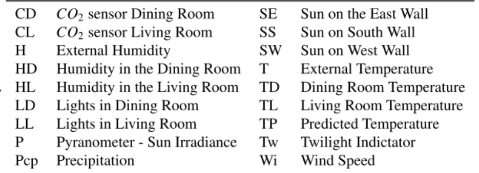
Spencer, Alfandi and Al-Obeidat / Procedia Computer Science 00 (2018) 000–000 5 Table 1: Sensors in the SML house

.

CD CO2sensor Dining Room SE Sun on the East Wall

CL CO2sensor Living Room SS Sun on South Wall

H External Humidity SW Sun on West Wall

HD Humidity in the Dining Room T External Temperature HL Humidity in the Living Room TD Dining Room Temperature

LD Lights in Dining Room TL Living Room Temperature

LL Lights in Living Room TP Predicted Temperature P Pyranometer - Sun Irradiance Tw Twilight Indictator

Pcp Precipitation Wi Wind Speed

There are two collections of data available. The first, SML1, was collected from March 13 to April 11, 2012. The second, SML2, was collected from April 18 to May 2, 2012. To each sensor, we give a short name listed in Table1.

In Figure1, we see that the maximal RMSE error measured per forecast hour is remarkably stable over the fore-cast horizon. Initially there is a very low forefore-cast error, which occurs because the forefore-cast temperature is influenced strongly by a few sensors, including the current temperature. We also see that the forecasted temperature is lower than about 1.3 Celsius degree from the observed temperature over the entire 48 hour period. Finally we can see that using MIDFEL LASSO regression, shown on the right, the results are almost identicl to LASSO regression, on the left. Somewhat surprising is that the forecasted temperature of the house remains quite accurate even beyond 24 hours. We surmise this is due to similarities in the daily routine adopted by the house occupants.

Fig. 1: Based on the dataset from the SML HouseA collected in March and April 2012, these plots show the maximal RMSE segmented by hour for 48 hours. The modeller uses only the most influential sensors per segment. as computed by best first search. The left plot uses LASSO regression, and right uses MIDFEL LASSO regression with a balance of 0.2.

4.1. Arising Questions

1. Is temperature forecasting improved by using influential sensors?

(7)

6 Spencer, Alfandi and Al-Obeidat / Procedia Computer Science 00 (2018) 000–000 3. Which strategy is better for tuning LASSO regression: 1SE or MIDFEL?

4. How does the selection of influential sensors change as the data changes over different time periods?

To answer the first question, in work reported previously[1], we computed the forecast error using all sensors in the SML1 dataset. When using all sensors, we had to refrain from using a large number historical readings because in this case, the number of predictors in the model becomes very large, which overwhelms LASSO regression. Thus, fewer historical readings per sensor often gave better forecast errors. This indicates that LASSO regression, alone, cannot perform as well as LASSO regression with selected influential sensors. By using LASSO regression with four hours of historical readings per sensor, we achieved our lowest MSE of 1.69◦_{C. By using LASSO regression with one hour}

of historical readings, we achieved our best RMSE of 2.21◦_{C, as shown in Table}₂_{. These are the largest errors in this}

table for SML1 data. We conclude that the use of influential sensors improves forecast accuracy.

Table 2: Forecast errors for the SML1 data set collected over about four weeks, and the SML2 data set, collected later over about two weeks. All models compute forecasts every 15 minutes over 48 hours. When using data from all sensors, the LASSO models were given only four hours of data for the the mean RMSE error, and one hour of data for maximal RMSE. In all other cases, models use 24 hours of data.

Sensors Selection Method Data λ Mean RMSE Max RMSE

All sensors SML1 1SE 1.69 2.21

Influential over forecast horizon SML1 1SE 1.43

SML1 MIDFEL 1.41

Influential by hourly segments SML1 1SE 1.08 1.31

SML1 MIDFEL 1.07 1.32

Influential over forecast horizon SML2 1SE 3.33

SML2 MIDFEL 3.11

Influential by hourly segments SML2 1SE 1.19 1.92

SML2 MIDFEL 1.11 1.89

In Table2we also show results that relate to the second question: is forecast accuracy improved by using influential sensors, when those sensors are specifically selected to be influential for a specific hour? In this table we see that for both datasets SML 1 and SML2, and for both λ tuning strategies, 1SE and MIDFEL, the temperature forecast has lower maximal RMSE when sensors are selected specifically for each hour.

For the third question, when tuning LASSO regression hyperparameters, we see that the accuracy when using MIDFEL is similar to the accuracy when using 1SE, paricularly for the SML1 data. However, for the SML2 data, MIDFEL tuning is clearly more accurate, both for mean RMSE and maximial RMSE. With SML2 data, the combined effect of using hourly segments and MIDFEL tuning, is a 42% decrease in error, from 3.33◦_{C to 1.89}◦_C.

For the SML1 house, the improvement of RMSE over LASSO regression by using influential sensors is 35%. The improvement using influential sensors along with MIDFEL LASSO regression is 36%. Finally, the improvement using influential sensors per segment along with MIDFEL regression is 40%.

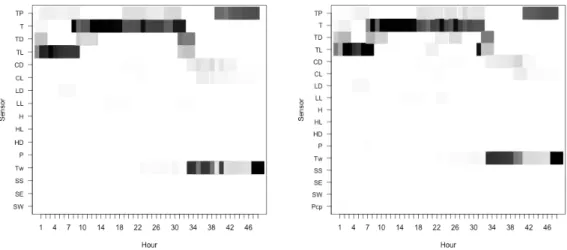
Considering the fourth question, in Figure2we present heatmaps indicating the magnitude of the coefficients for the sensors. There is one grey area for each sensor and for each hour of the forecast horizon. A darker grey area means the coefficient is larger, so that sensor is more influential.

The first two heatmaps are for the SML1 data. They appear quite similar. This indicates that 1SE and MIDFEL tuning have similar effects for this data. The third and fourth heatmaps show the coefficients assigned to the SML2 data. They are slightly different from each other, indicating that 1SE and MIDFEL tuning have different effects.

The most striking finding for the fourth question is that the influential sensors for the SML1 data are a close match for the most influential sensors for the SML2 data, although the SML1 plots are have fewer light and medium shades of grey. We cannot conclude from this that the sensors deemed to be influential, remain influential. Recall that the SML2 data set was collected over about half the time of the SML1 data set. Experiments are planned to investigate further. If we find that the influential sensors, once computed, can be reused in future periods, we could avoid repeating an expensive operation.

We hypothesize that amount of grey in the coefficient heatmap gives some indication of the error. The SML2 heatmaps feature more grey-scaled areas than the SML1 areas. Correspondingly, the SML2 models generate a higher

(8)

Bruce Spencer et al. / Procedia Computer Science 155 (2019) 511–518 517

(a) Heatmaps showing the coefficients for the SML1 data, using 1SE tuning and MIDFEL tuning, respectively.

(b) Heatmaps showing the coefficents from SML2 data and again they use 1SE and MIDFEL tuning, respectively.

Fig. 2: These heatmaps show the influence attributed to each sensor by LASSO regression, where darker grey indicates more influence.

error than the SML1 models. For more evidence, notice that between the two SML2 models, the 1SE model has more grey areas, and has a higher error. It appears that only five sensors are very influential for the SML1 data, namely TP, T, TD, TL and Tw, and only certain periods for these are important. Based on these observations, we hypothesize that a very simple linear model can serve to generate highly accurate forecasts.

5. Conclusion

We address the following problem: We are given a physical system that is influenced by events, where these events are indicted by values that can be read from sensors. We are asked to forecast the value of an attribue of interest, which itself is reported by a sensor. We are presented with the sensors readings over a period of time and asked to predict the value of the attribute of interest over some future period of time. Specifically we want to forecast the internal temperature of a dwelling so that we can apply more intelligent control of heating and cooling systems, and so reduce energy usage.

(9)

In our model we seek to reduce the complexity of the model by exploiting the fact that different events may affect the attribute of interest at different times in the future.

We propose a trio of techniques that work together to address this problem. Two of the technologies, namely the selection of influential sensors and MIDFEL LASSO regression, have previously been presented. A new technique uses these two previous ones to select the most influential sensors over each segment of the forecast horizon.

Using sensor data from a smart house, we illustrate how the three techniques work together. The combination provides improves forecast accuracy.

We also show that the selection of most influential sensors is somewhat stable over different modelling techniques and bears some similarity over data gathered from the same house over a different time period.

Segmenting and tuning in this work has provided a surprisingly clear picture of which observations from which sen-sors should be used to forecast temperature at a future time. With more data, the picture’s clarity increases, suggesting that being influential could be a stable property, and so it can be used to improve accuracy over many periods. Acknowledgements

The authors acknowledge the support of their organizations. Special thanks to Zayed University for RIF fund 17063 and to ComputeCanada.ca for computing facilities.

References

[1] Al-Obeidat, F., Spencer, B., Alfandi, O., 2018. Consistently accurate forecasts of temperature within buildings from sensor data using ridge and lasso regression. Future Generation Computer Systems .

[2] ´Alvarez, J., Redondo, J., Camponogara, E., Normey-Rico, J., Berenguel, M., Ortigosa, P., 2013. Optimizing building comfort temperature regulation via model predictive control. Energy and Buildings 57, 361 – 372.

[3] Friedman, J., Hastie, T., Simon, N., Tibshirani, R., 2016. Package glmnet: Lasso and Elastic-Net Regularized Generalized Linear Models Ver 2.0-.https://cran.r-project.org/web/packages/glmnet/glmnet.pdf.

[4] Friedman, J., Hastie, T., Tibshirani, R., 2010. Regularization paths for generalized linear models via coordinate descent. Journal of Statistical Software 33, 1–22. URL:http://www.jstatsoft.org/v33/i01/.

[5] Morosan, P., Bourdais, R., Dumur, D., Buisson, J., 2010. Building temperature regulation using a distributed model predictive control. Energy and Buildings , 1445–1452.

[6] P´erez-Lombard, L., Ortiz, J., Pout, C., 2008. A review on buildings energy consumption information. Energy and Buildings 40, 394–398. [7] Romanski, P., Kotthoff, L., 2016a. FSelector: Selecting Attributes. R package version 0.21.

[8] Romanski, P., Kotthoff, L., 2016b. Package ‘FSelector’ Selecting Attributes. R package version 0.21. https://cran.r-project.org/web/packages/FSelector/FSelector.pdf.

[9] Simon, N., Friedman, J., Hastie, T., Tibshirani, R., 2011. Regularization paths for cox’s proportional hazards model via coordinate descent. Journal of Statistical Software 39, 1–13. URL:http://www.jstatsoft.org/v39/i05/.

[10] Spencer, B., Al-Obeidat, F., Alfandi, O., 2016. Short term forecasts of internal temperature with stable accuracy in smart homes. International Journal of Thermal and Environmental Engineering 13, 81–89.

[11] Spencer, B., Al-Obeidat, F., Alfandi, O., 2017a. Accurately forecasting temperatures in smart buildings using fewer sensors. Personal and Ubiquitous Computing URL:https://doi.org/10.1007/s00779-017-1103-4, doi:10.1007/s00779-017-1103-4.

[12] Spencer, B., Al-Obeidat, F., Alfandi, O., 2017b. Selecting sensors when forecasting temperature in smart buildings. Procedia Computer Science 109, 777 – 784. URL:http://www.sciencedirect.com/science/article/pii/S1877050917309857, doi:https://doi. org/10.1016/j.procs.2017.05.321. 8th International Conference on Ambient Systems, Networks and Technologies, ANT-2017 and the 7th International Conference on Sustainable Energy Information Technology, SEIT 2017, 16-19 May 2017, Madeira, Portugal.

[13] Spencer, B., Alfandi, O., Al-Obeidat, F., 2018. A refinement of lasso regression applied to temperature forecasting. Procedia Computer Science 130, 728 – 735. URL:http://www.sciencedirect.com/science/article/pii/S1877050918304897, doi:https://doi.org/10. 1016/j.procs.2018.04.127. the 9th International Conference on Ambient Systems, Networks and Technologies (ANT 2018) / The 8th International Conference on Sustainable Energy Information Technology (SEIT-2018) / Affiliated Workshops.

[14] Tibshirani, R., 1996. Regression shrinkage and selection via the lasso: a retrospective. Journal of the Royal Statistical Society: Series B (Statistical Methodology) 58, 267–288. URL:http://www.jstor.org/stable/2346178.

[15] UCI, 2010. Sml2010 data set.https://archive.ics.uci.edu/ml/datasets/SML2010.

[16] Zamora-Mart´ınez, F., Romeu, P., Botella-Rocamora, P., Pardo, J., 2013. Towards energy efficiency: Forecasting indoor temperature via multi-variate analysis. Energies 6, 4639. URL:http://www.mdpi.com/1996-1073/6/9/4639, doi:10.3390/en6094639.

[17] Zamora-Mart´ınez, F., Romeu, P., Botella-Rocamora, P., Pardo, J., 2014. On-line learning of indoor temperature forecasting models towards energy efficiency. Energy and Buildings 83, 162–172.