Measurement of jet shapes in top-quark pair events at sqrt(s) = 7 TeV using the ATLAS detector

(1)

EUROPEAN ORGANISATION FOR NUCLEAR RESEARCH (CERN)

CERN-PH-EP-2013-067

Submitted to: Eur. Phys. J. C

Measurement of jet shapes in top pair events at

√

s

= 7 TeV using

the ATLAS detector

The ATLAS Collaboration

Abstract

A measurement of jet shapes in top-quark pair events using 1.8 fb

−1

of

√

s

= 7 TeV pp collision

data recorded by the ATLAS detector at the LHC is presented. Samples of top-quark pair events are

selected in both the single-lepton and dilepton final states. The differential and integrated shapes of

the jets initiated by bottom-quarks from the top-quark decays are compared with those of the jets

originated by light-quarks from the hadronic W -boson decays W

_{→ q ¯q}

0

_{in the single-lepton channel.}

The light-quark jets are found to have a narrower distribution of the momentum flow inside the jet area

than b-quark jets.

(2)

(will be inserted by the editor)

Measurement of jet shapes in top-quark pair events at

√

s

= 7 TeV using

the ATLAS detector

The ATLAS Collaboration

1

1_{CERN, 1211 Geneva 23, Switzerland}

Received: date / Accepted: date

Abstract A measurement of jet shapes in top-quark pair

events using 1.8 fb

−1

of

√

s

= 7 TeV pp collision data

recor-ded by the ATLAS detector at the LHC is presented.

Sam-ples of top-quark pair events are selected in both the

single-lepton and disingle-lepton final states. The differential and

inte-grated shapes of the jets initiated by bottom-quarks from the

top-quark decays are compared with those of the jets

orig-inated by light-quarks from the hadronic W -boson decays

W

_{→ q ¯q}

0

in the single-lepton channel. The light-quark jets

are found to have a narrower distribution of the momentum

flow inside the jet area than b-quark jets.

1 Introduction

Hadronic jets are observed in large momentum-transfer

in-teractions. They are theoretically interpreted to arise when

partons – quarks (q) and gluons (g) – are emitted in

colli-sion events of subatomic particles. Partons then evolve into

hadronic jets in a two-step process. The first can be

de-scribed by perturbation theory and gives rise to a parton

shower, the second is non-perturbative and is responsible

for the hadronisation. The internal structure of a jet is

ex-pected to depend primarily on the type of parton it originated

from, with some residual dependence on the quark

produc-tion and fragmentaproduc-tion process. For instance, due to the

di-fferent colour factors in ggg and qqg vertices, gluons lead to

more parton radiation and therefore gluon-initiated jets are

expected to be broader than quark-initiated jets.

For jets defined using cone or k

t

algorithms [1, 2], jet shapes,

i.e. the normalised transverse momentum flow as a function

of the distance to the jet axis [3], have been traditionally

used as a means of understanding the evolution of partons

into hadrons in e

+

e

−

, ep and hadron colliders [4–11]. It is

experimentally observed that jets in e

+

e

−

and ep are

nar-rower than those observed in p ¯

p

and pp collisions and this

is interpreted as a result of the different admixtures of quark

and gluon jets present in these different types of

interac-tions [12]. Furthermore, at high momentum transfer, where

fragmentation effects are less relevant, jet shapes have been

found to be in qualitative agreement with

next-to-leading-order (NLO) QCD predictions and in quantitative agreement

with those including leading logarithm corrections [13]. Jet

shapes have also been proposed as a tool for studies of

sub-structure or in searches for new phenomena in final states

with highly boosted particles [14–17].

Due to the mass of the quark, jets originating from a

b-quark (hereafter called b-jets) are expected to be broader

than light-quark jets, including charm jets, hereafter called

light jets. This expectation is supported by observations by

the CDF collaboration in Ref. [18], where a comparison is

presented between jet shapes in a b-jet enriched sample with

a purity of roughly 25% and an inclusive sample where no

distinction is made between the flavours.

This paper presents the first measurement of b-jet shapes in

top pair events. The t ¯t final states are a source of b-jets, as

the top quark decays almost exclusively via t

_{→ W b. While}

the dilepton channel, where both W bosons decay to leptons,

is a very pure source of b-jets, the single-lepton channel

contains b-jets and light jets, the latter originating from the

dominant W

+

_{→ u ¯}

d, c ¯s decays and their charge conjugates.

A comparison of the light- and b-jet shapes measured in the

t ¯t

decays improves the CDF measurement discussed above,

as the jet purity achieved using t ¯t events is much higher. In

addition, these measurements could be used to improve the

modelling of jets in t ¯t production Monte Carlo (MC) models

in a new kinematic regime.

This paper is organised as follows. In Sect. 2 the ATLAS

detector is described, while Sect. 3 is dedicated to the MC

samples used in the analysis. In Sects. 4 and 5, the physics

object and event selection for both the dilepton and

single-lepton t ¯t samples is presented. Section 6 is devoted to the

(3)

description of both the b-jet and light-jet samples obtained

in the single-lepton final state. The differential and the

inte-grated shape distributions of these jets are derived in Sect. 7.

In Sect. 8 the results on the average values of the jet shape

variables at the detector level are presented, including those

for the b-jets in the dilepton channel. Results corrected for

detector effects are presented in Sect. 9. In Sect. 10 the

sys-tematic uncertainties are discussed, and Sect. 11 contains a

discussion of the results. Finally, Sect. 12 includes the

sum-mary and conclusions.

2 The ATLAS detector

The ATLAS detector [19] is a multi-purpose particle physics

detector with a forward-backward symmetric cylindrical

ge-ometry

1

and a solid angle coverage of almost 4π.

The inner tracking system covers the pseudorapidity range

|η| < 2.5, and consists of a silicon pixel detector, a

sili-con microstrip detector, and, for

_{|η| < 2.0, a transition}

ra-diation tracker. The inner detector (ID) is surrounded by

a thin superconducting solenoid providing a 2 T magnetic

field along the beam direction. A high-granularity

liquid-argon sampling electromagnetic calorimeter covers the

re-gion

_{|η| < 3.2. An iron/scintillator tile hadronic}

calorime-ter provides coverage in the range

_{|η| < 1.7. The endcap}

and forward regions, spanning 1.5 <

_{|η| < 4.9, are}

instru-mented with liquid-argon calorimeters for electromagnetic

and hadronic measurements. The muon spectrometer

sur-rounds the calorimeters. It consists of three large air-core

su-perconducting toroid systems and separate trigger and

high-precision tracking chambers providing accurate muon

track-ing for

_{|η| < 2.7.}

The trigger system [20] has three consecutive levels: level

1 (L1), level 2 (L2) and the event filter (EF). The L1

trig-gers are hardware-based and use coarse detector

informa-tion to identify regions of interest, whereas the L2 triggers

are based on fast software-based online data reconstruction

algorithms. Finally, the EF triggers use offline data

recon-struction algorithms. For this analysis, the relevant triggers

select events with at least one electron or muon.

3 Monte Carlo Samples

Monte Carlo generators are used in which t ¯t production is

implemented with matrix elements calculated up to NLO

ac-1_{ATLAS uses a right-handed coordinate system with its origin at the}

nominal interaction point (IP) in the centre of the detector and the z-axis along the beam pipe. The x-z-axis points from the IP to the centre of the LHC ring, and the y-axis points upward. Cylindrical coordinates (r, φ ) are used in the transverse plane, φ being the azimuthal angle around the beam pipe. The pseudorapidity is defined in terms of the

polar angle θ as η=−lntan(θ/2).

curacy. The generated events are then passed through a

de-tailed GEANT4 simulation [21, 22] of the ATLAS detector.

The baseline MC samples used here are produced with the

MC@NLO [23] or POWHEG

[24] generators for the

ma-trix element calculation; the parton shower and

hadronisa-tion processes are implemented with HERWIG

[25] using the

cluster hadronisation model [26] and CTEQ6.6 [27] parton

distribution functions (PDFs). Multi-parton interactions are

simulated using JIMMY

[28] with the AUET1 tune [29]. This

MC generator package has been used for the description of

the t ¯t final states for ATLAS measurements of the cross

sec-tion [30, 31] and studies of the kinematics [32].

Additional MC samples are used to check the

hadronisa-tion model dependence of the jet shapes. They are based

on POWHEG+PYTHIA

[24, 33], with the MRST2007LO*

PDFs [34]. The ACERMC generator [35] interfaced to

PY-THIA

with the PERUGIA

2010 tune [36] for parton

shower-ing and hadronisation is also used for comparison. Here the

parton showers are ordered by transverse momentum and the

hadronisation proceeds through the Lund string

fragmenta-tion scheme [37]. The underlying event and other soft effects

are simulated by PYTHIA

with the AMBT1 tune [38].

Com-parisons of different event generators show that jet shapes in

top-quark decays show little sensitivity to initial-state

radi-ation effects, different PDF choices or underlying-event

ef-fects. They are more sensitive to details of the parton shower

and the fragmentation scheme.

Samples of events including W and Z bosons produced in

association with light- and heavy-flavour jets are generated

using the ALPGEN

[39] generator with the CTEQ6L PDFs

[40], and interfaced with HERWIG

and JIMMY. The same

generator is used for the diboson backgrounds, WW , W Z

and ZZ, while MC@NLO is used for the simulation of the

single-top backgrounds, including the t- and s-channels as

well as the W t-channel.

The MC-simulated samples are normalised to the

correspon-ding cross sections. The t ¯t signal is normalised to the cross

section calculated at approximate next-to-next-to-leading

or-der (NNLO) using the HATHOR

package [41], while for the

single-top production cross section, the calculations in Refs.

[42–44] are used. The W +jets and Z+jets cross sections are

taken from ALPGEN

[39] with additional NNLO K-factors

as given in Ref. [45].

The simulated events are weighted such that the distribution

of the number of interactions per bunch crossing in the

sim-ulated samples matches that of the data. Finally, additional

correction factors are applied to take into account the

di-fferent object efficiencies in data and simulation. The scale

factors used for these corrections tipically differ from unity

by 1% for electrons and muons, and by a few percent for

b-tagging.

(4)

4 Physics object selection

Electron candidates are reconstructed from energy deposits

in the calorimeter that are associated with tracks

reconstruc-ted in the ID. The candidates must pass a tight selection

[46], which uses calorimeter and tracking variables as well

as transition radiation for

_{|η| < 2.0, and are required to have}

transverse momentum pT

> 25 GeV and

_{|η| < 2.47.}

Elec-trons in the transition region between the barrel and endcap

calorimeters, 1.37 <

|η| < 1.52, are not considered.

Muon candidates are reconstructed by searching for track

segments in different layers of the muon spectrometer. These

segments are combined and matched with tracks found in

the ID. The candidates are refitted using the complete track

information from both detector systems and are required to

have a good fit and to satisfy p

T

> 20 GeV and

|η| < 2.5.

Electron and muon candidates are required to be isolated to

reduce backgrounds arising from jets and to suppress the

se-lection of leptons from heavy-flavour semileptonic decays.

For electron candidates, the transverse energy deposited in

the calorimeter and which is not associated with the

elec-tron itself (E

_Tiso

) is summed in a cone in η

_{− φ space of}

ra-dius

2

∆ R

= 0.2 around the electron. The E

_Tiso

value is

re-quired to be less than 3.5 GeV. For muon candidates, both

the corresponding calorimeter isolation E

_Tiso

and the

anal-ogous track isolation transverse momentum (p

iso_T

) must be

less than 4 GeV in a cone of ∆ R

= 0.3. The track isolation

is calculated from the scalar sum of the transverse momenta

of tracks with p

T

> 1 GeV, excluding the muon.

Muon candidates arising from cosmic rays are rejected by

removing candidate pairs that are back-to-back in the

trans-verse plane and that have transtrans-verse impact parameter

rela-tive to the beam axis

_|d

0

| > 0.5 mm.

Jets are reconstructed with the anti-k

t

algorithm [47, 48]

with radius parameter R

= 0.4. This choice for the radius has

been used in measurements of the top-quark mass [49] and

also in multi-jet cross-section measurements [50]. The

in-puts to the jet algorithm are topological clusters of

calorime-ter cells. These cluscalorime-ters are seeded by calorimecalorime-ter cells with

energy

_|E

cell

| > 4σ , where σ is the cell-by-cell RMS of the

noise (electronics plus pileup). Neighbouring cells are added

if

_{|Ecell| > 2σ and clusters are formed through an iterative}

procedure [51]. In a final step, all remaining neighbouring

cells are added to the cluster.

The baseline calibration for these clusters calculates their

energy using the electromagnetic energy scale [54]. This

is established using test-beam measurements for electrons

and muons in the electromagnetic and hadronic

calorime-ters [51–53]. Effects due to the differing response to

electro-magnetic and hadronic showers, energy losses in the dead

material, shower leakage, as well as inefficiencies in energy

clustering and jet reconstruction are also taken into account.

2_{The radius in the η}_{− φ space is defined as ∆R =}_p(∆η)2_{+ (∆ φ )}2

This is done by matching calorimeter jets with MC particle

jets in bins of η and E, and supplemented by in situ

calibra-tion methods such as jet momentum imbalance in Z/γ

∗

+ 1

jet events. This is called the Jet Energy Scale (JES)

calibra-tion, thoroughly discussed in Ref. [54]. The JES uncertainty

contains an extra term for b-quark jets, as the jet response is

different for b-jets and light jets because they have different

particle composition. References [50] and [55] contain more

details on the JES and a discussion of its uncertainties.

Jets that overlap with a selected electron are removed if they

are closer than ∆ R

= 0.2, while if a jet is closer than ∆ R =

0.4 to a muon, the muon is removed.

The primary vertex is defined as the pp interaction vertex

with the largest ∑i

p

2_Ti

, where the sum runs over the tracks

with p

T

> 150 MeV associated with the vertex.

Jets are identified as candidates for having originated from

a b-quark (b-tagged) by an algorithm based on a

neural-network approach, as discussed in Sect. 6.

The reconstruction of the direction and magnitude (E

_Tmiss

) of

the missing transverse momentum is described in Ref. [56]

and begins with the vector sum of the transverse momenta of

all jets with p

T

> 20 GeV and

|η| < 4.5. The transverse

mo-menta of electron candidates are added. The contributions

from all muon candidates and from all calorimeter clusters

not belonging to a reconstructed object are also included.

5 Event selection

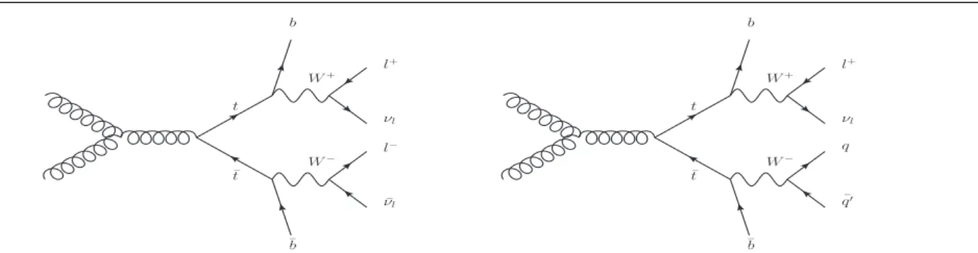
Two samples of events are selected: a dilepton sample, where

both W bosons decay to leptons (e, µ, including leptonic τ

decays), and a single-lepton sample, where one W boson

decays to leptons and the other to a q ¯

q

0

pair, giving rise

to two more jets (see Fig. 1). The selection criteria follow

those in Ref. [30] for the single-lepton sample and Ref. [31]

for the dilepton sample. Events are triggered by inclusive

high-p

T

electron or muon EF triggers. The trigger

thresh-olds are 18 GeV for muons and 20 GeV for electrons. The

dataset used for the analysis corresponds to the first half

of the data collected in 2011, with a centre-of-mass energy

√

_s

_{= 7 TeV and an integrated luminosity of 1.8 fb}

₋₁

_{. This}

data-taking period is characterised by an instantaneous

lumi-nosity smaller than 1.5

_×10

33

_cm

−2

_s

−1

_{, for which the mean}

number of interactions per bunch crossing is less than six. To

reject the non-collision background, the primary vertex is

re-quired to have at least four tracks, each with p

T

> 150 MeV,

associated with it. Pile-up effects are therefore small and

have been taken into account as a systematic uncertainty.

5.1 Dilepton sample

In the dilepton sample, events are required to have two

char-ged leptons and E

_Tmiss

from the leptonic W -boson decays

(5)

t ¯ t b ¯ b W+ W− l+ νl l− ¯ νl t ¯ t b ¯b W+ W− l+ νl q ¯ q′

Fig. 1 Example LO Feynman diagrams for gg→ t¯t in the dilepton (left) and single-lepton (right) decay modes.

to a neutrino and an electron or muon. The offline lepton

selection requires two isolated leptons (e or µ) with

oppo-site charge and with transverse momenta p

T(e) > 25 GeV,

where p

T(e) = Ecluster

sin(θ

track

), E

cluster

being the

clus-ter energy and θ

track

the track polar angle, and p

T(µ) >

20 GeV. At least one of the selected leptons has to match

the corresponding trigger object.

Events are further filtered by requiring at least two jets with

pT

> 25 GeV and

_{|η| < 2.5 in the event. In addition, at least}

one of the selected jets has to be tagged as a b-jet, as

dis-cussed in the next section. The whole event is rejected if a

jet is identified as an out-of-time signal or as noise in the

calorimeter.

The missing transverse momentum requirement is E

_Tmiss

>

60 GeV for the ee and µ µ channels. For the eµ channel,

H

T

is required to be greater than 130 GeV, where H

T

is the

scalar sum of the p

T

of all muons, electrons and jets. To

reject the Drell–Yan lepton pair background in the ee and

µ µ channels, the lepton pair is required to have an

invari-ant mass m

``

greater than 15 GeV and to lie outside of a

Z-boson mass window, rejecting all events where the

two-lepton invariant mass satisfies

_|m``

_{− m}

Z

| < 10 GeV.

The selected sample consists of 95% t ¯t events, but also

back-grounds from the final states W + jets and Z + jets, where the

gauge bosons decay to leptons. All backgrounds, with the

exception of multi-jet production, have been estimated using

MC samples. The multi-jet background has been estimated

using the jet–electron method [60]. This method relies on

the identification of jets which, due to their high

electro-magnetic energy fraction, can fake electron candidates. The

jet–electron method is applied with some modifications to

the muon channel as well. The normalisation is estimated

using a binned likelihood fit to the E

_Tmiss

distribution. The

results are summarised in Table 1.

5.2 Single-Lepton sample

In this case, the event is required to have exactly one isolated

lepton with p

T

> 25 GeV for electrons and pT

> 20 GeV

for muons. To account for the neutrino in the leptonic W

Table 1 The expected composition of the dilepton sample. Fractions are relative to the total number of expected events. ‘Other EW’ corre-sponds to the W + jets and diboson (WW , W Z and ZZ) contributions.

Process Expected events Fraction

t ¯t 2100± 110 94.9% Z+ jets (Z_{→ `}+`−) 14_{± 1} 0.6% Other EW (W , diboson) 4_{± 2} 0.2% Single top 95_{± 2} 4.3% Multi-jet 0+2₋₀ 0.0% Total Expected 2210± 110 Total Observed 2067

decay, E

_Tmiss

is required to be greater than 35 GeV in the

electron channel and greater than 20 GeV in the muon

chan-nel. The E

_Tmiss

resolution is below 10 GeV [56].

Further-more, the transverse mass

3

(m

T

) is required to be greater

than 25 GeV in the e-channel and to satisfy the condition

E

_Tmiss

+ mT

> 60 GeV in the µ-channel.

The jet selection requires at least four jets (p

T

> 25 GeV

and

_{|η| < 2.5) in the final state, and at least one of them}

has to be tagged as a b-jet. The fraction of t ¯t events in the

sample is 77%; the main background contributions for the

single-lepton channel have been studied as in the previous

case, and are summarised in Table 2. As in the dileptonic

case, the multi-jet background has been estimated using the

jet–electron method.

6 Jet sample definition

Jets reconstructed in the single-lepton and dilepton samples

are now subdivided into b-jet and light-jet samples. In order

to avoid contributions from non-primary collisions, it is

re-quired that the jet vertex fraction (JVF) be greater than 0.75.

After summing the scalar p

T

of all tracks in a jet, the JVF is

defined as the fraction of the total scalar p

T

that belongs to

3_{The transverse mass is defined as m}

T=

q

2p`_TE_Tmiss(1− cos∆φ`ν),

where ∆ φ`νis the angle in the transverse plane between the selected

lepton and the Emiss

(6)

Table 2 The expected composition of the single-lepton sample. Frac-tions are relative to the total number of expected events. In this case ‘Other EW’ includes Z + jets and diboson processes.

Process Expected events Fraction

t ¯t 14000_{± 700} 77.4% W+ jets (W_{→ `ν)} 2310_{± 280} 12.8% Other EW (Z, diboson) 198_{± 18} 1.1% Single top 668_{± 14} 3.7% Multi-jet 900_{± 450} 5.0% Total Expected 18000_{± 900} Total Observed 17019

tracks originating from the primary vertex. This makes the

average jet multiplicity independent of the number of pp

in-teraction vertices. This selection is not applied to jets with

no associated tracks. Also, to reduce the impact of pileup on

the jets, the p

T

threshold has been raised to 30 GeV.

Jets whose axes are closer than ∆ R

= 0.8, which is twice

the jet radius, to some other jet in the event are not

consid-ered. This is done to avoid possible overlaps between the jet

cones, which would bias the shape measurement. These

con-figurations are typical in boosted W bosons, leading to light

jets which are not well separated. The resulting ∆ R

distri-butions for any pair of b-jets or light jets are approximately

constant between 0.8 and π and exhibit an exponential

fall-off between π and the endpoint of the distribution.

6.1 b-jet samples

To select b-jets, a neural-network algorithm, which relies on

the reconstruction of secondary vertices and impact

parame-ter information in the three spatial dimensions, is used. The

reconstruction of the secondary decay vertices makes use of

an iterative Kalman-filter algorithm [61] which relies on the

hypothesis that the b

_{→ c → X decay chains lie in a straight}

line originally taken to be parallel to the jet axis. The

work-ing point of the algorithm is chosen to maximise the

pu-rity of the sample. It corresponds to a b-tagging efficiency

of 57% for jets originating from b-quarks in simulated t ¯t

events, and a u, d, s-quark jet rejection factor of about 400,

as well as a c-jet rejection factor of about 10 [62, 63]. The

resulting number of b-jets selected in the dilepton

(single-lepton) sample is 2279 (16735). A second working point

with a b-tagging efficiency of 70% is also used in order to

evaluate the dependence of the measured jet shapes on

b-tagging.

Figure 2 shows the b-tagged jet transverse momentum

distri-butions for the single-lepton and dilepton channels. The pT

distributions for the b-jets in both the dilepton and

single-lepton samples show a similar behaviour, since they come

mainly from top-quark decays. This is well described by the

[GeV] T p 0 50 100 150 200 250 300 350 Jets / 10 GeV 500 1000 1500 2000 2500 = 7 TeV s Data t t ν l → W Multi-jet Other EW Single top

ATLAS

Single lepton

∫

L dt = 1.8 fb-1 [GeV] T p 0 50 100 150 200 250 300 350 Jets / 10 GeV 50 100 150 200 250 300 350 = 7 TeV s Data t t l + l → Z Other EW Single top

ATLAS

Dilepton

∫

L dt = 1.8 fb-1

Fig. 2 The pTdistributions for b-tagged jets in the single-lepton (top)

and dilepton (bottom) samples along with the sample composition ex-pectations.

MC expectations from the MC@NLO generator coupled to

HERWIG. In the dilepton sample the signal-to-background

ratio is found to be greater than in the single-lepton sample,

as it is quantitatively shown in Tables 1 and 2.

6.2 Light-quark jet sample

The hadronic decays W

_{→ q ¯q}

0

are a clean source of

light-quark jets, as gluons and b-jets are highly suppressed; the

former because gluons would originate in radiative

correc-tions of order

O(αs), and the latter because of the smallness

of the CKM matrix elements

_|V

ub

| and |V

cb

|. To select the

light-jet sample, the jet pair in the event which has the

in-variant mass closest to the W -boson mass is selected. Both

jets are also required to be non-tagged by the b-tagging

al-gorithm. The number of jets satisfying these criteria is 7158.

Figure 3 shows the transverse momentum distribution of

these jets together with the invariant mass of the dijet

sys-tem. As expected, the p

T

distribution of the light jets from

W

-boson decays exhibits a stronger fall-off than that for the

(7)

[GeV] T p 0 50 100 150 200 250 Jets / 10 GeV 200 400 600 800 1000 1200 1400 1600 1800 2000 2200 2400 = 7 TeV s Data t t ν l → W Multi-jet Other EW Single top

ATLAS

-1 L dt = 1.8 fb

∫

[GeV] jj m 0 20 40 60 80 100 120 140 Events / 4 GeV 200 400 600 800 1000 = 7 TeV s Data t t ν l → W Multi-jet Other EW Single top

ATLAS

-1 L dt = 1.8 fb

∫

Fig. 3 The distribution of light-jet pT(top) and of the invariant mass

of light-jet pairs (bottom) along with the sample composition expec-tations. The latter shows a peak at the W mass, whose width is deter-mined by the dijet mass resolution.

b-jets. This dependence is again well described by the MC

simulations in the jet p

T

region used in this analysis.

Agree-ment between the invariant mass distributions for observed

and simulated events is good, in particular in the region close

to the W -boson mass.

6.3 Jet purities

To estimate the actual number of b-jets and light jets in each

of the samples, the MC simulation is used by analysing the

information at generator level. For jets, a matching to a

b-hadron is performed within a radius ∆ R

= 0.3. For light jets,

the jet is required not to have a b-hadron within ∆ R

= 0.3

of the jet axis. Additionally, to distinguish light quarks and

c-quarks from gluons, the MC parton with highest pT

within

the cone of the reconstructed jet is required to be a (u, d, c or

s)-quark. The purity p is then defined as

p

=

_∑

k

α

k

p

k

;

p

k

= 1

−

N

_f(k)

N

_T(k)

(1)

Table 3 Purity estimation for b-jets and light jets in the single-lepton channel. The uncertainty on the purity arises from the uncertainties in the signal and background fractions.

Process αk pk(b) pk(light) t ¯t 0.774 0.961 0.725 W_{→ `ν} 0.128 0.430 0.360 Multi-jet 0.050 0.887 0.485 Other EW (Z, diboson) 0.011 0.611 0.342 Single top 0.037 0.958 0.716 Weighted total - (88.5± 5.7)% (66.2± 4.1)%

Table 4 Purity estimation for b-jets in the dilepton channel. The un-certainty on the purity arises from the uncertainties in the signal and background fractions. Process αk pk(b) t ¯t 0.949 0.997 Z_{→ `}+`− _0.006 _0.515 Other EW (W , diboson) 0.002 0.375 Single top 0.043 0.987 Multi-jet - -Weighted total - (99.3+0.7 −6.5)%

where α

k

is the fraction of events in the k-th MC sample

(signal or background), given in Tables 1 and 2 and N

_f(k)

,

N

_T(k)

are the number of fakes (jets not assigned to the correct

flavour, e.g. charm jets in the b-jet sample), and the total

number of jets in a given sample, respectively. The purity in

the multi-jet background is determined using PYTHIA

MC

samples.

In the single-lepton channel, the resulting purity of the b-jet

sample is p

(s)_b

= (88.5

_{±5.7)%, while the purity of the}

light-jet sample is found to be p

(s)_l

= (66.2

± 4.1)%, as shown in

Table 3. The uncertainty on the purity arises from the

un-certainties on the signal and background fractions in each

sample. The charm content in the light-jet sample is found

to be 16%, with the remaining 50% ascribed to u, d and s.

MC studies indicate that the contamination of the b-jet

sam-ple is dominated by charm-jet fakes and that the gluon

con-tamination is about 0.7%. For the light-jet sample, the

frac-tion of gluon fakes amounts to 19%, while the b-jet fakes

correspond to 15%.

In the dilepton channel, a similar calculation yields the

pu-rity of the b-jet sample to be p

(d)_b

= (99.3

+0.7_−6.5

)% as shown

in Table 4. Thus, the b-jet sample purity achieved using t ¯t

fi-nal states is much higher than that obtained in inclusive b-jet

measurements at the Tevatron [18] or the LHC [55].

(8)

0 5 10 15 20 25

Jets / 1.0

1 10 2 10 3 10 4 10 _ATLAS _s_{= 7 TeV} r = 0.02 1 10 2 3 4 -1 L dt = 1.8 fb

∫

r = 0.10 0 5 10 15 20 25

Jets / 1.0

1 10 2 10 3 10 4 10 r = 0.18 (r) ρ 0 5 10 15 20 25 1 10 2 3 4 r = 0.26 (r) ρ 0 5 10 15 20 25

Jets / 1.0

1 10 2 10 3 10 4 10 r = 0.34 _Data t t ν l → W Multi-jet Other EW Single top

Fig. 4 Distribution of R= 0.4 b-jets in the single-lepton channel as a

function of the differential jet shapes ρ(r) for different values of r.

7 Jet shapes in the single-lepton channel

For the jet shape calculation, locally calibrated topological

clusters are used [54, 57, 58]. In this procedure, effects due

to calorimeter response, leakage, and losses in the dead

ma-terial upstream of the calorimeter are taken into account

sep-arately for electromagnetic and hadronic clusters [59].

The differential jet shape ρ

(r) in an annulus of inner radius

r

_{− ∆r/2 and outer radius r + ∆r/2 from the axis of a given}

jet is defined as

ρ

(r) =

1 ∆ r

pT(r

− ∆r/2,r + ∆r/2)

p

T(0, R)

(2)

Here, ∆ r

= 0.04 is the width of the annulus; r, such that

∆ r/2

_{≤ r ≤ R − ∆r/2, is the distance to the jet axis in the}

η -φ plane, and pT(r1, r2) is the scalar sum of the pT

of the

jet constituents with radii between r

1

and r

2

.

Some distributions of ρ(r) are shown in Fig. 4 for the

b-jet sample selected in the single-lepton channel. There is a

marked peak at zero energy deposit, which indicates that

en-ergy is concentrated around relatively few particles. As r

in-creases, the distributions of ρ

(r) are concentrated at smaller

values because of the relatively low energy density at the

pe-riphery of the jets. Both effects are well reproduced by the

0 5 10 15 20 25

Jets / 1.0

∫

r = 0.10 0 5 10 15 20 25

Jets / 1.0

1 10 2 10 3 10 4 10 r = 0.18 (r) ρ 0 5 10 15 20 25 1 10 2 3 4 r = 0.26 (r) ρ 0 5 10 15 20 25

Jets / 1.0

1 10 2 10 3 10 4 10 r = 0.34 _Data t t ν l → W Multi-jet Other EW Single top

Fig. 5 Distribution of R= 0.4 light jets in the single-lepton channel as

a function of the differential jet shapes ρ(r) for different values of r.

MC generators.

The analogous ρ(r) distributions for light jets are shown in

Fig. 5. The gross features are similar to those previously

dis-cussed for b-jets, but for small values of r, the ρ(r)

distribu-tions for light jets are somewhat flatter than those for b-jets.

The integrated jet shape in a cone of radius r

_{≤ R around the}

jet axis is defined as the cumulative distribution for ρ(r), i.e.

Ψ(r) =

pT(0, r)

p

T(0, R)

; r

≤ R

(3)

which satisfies Ψ(r = R) = 1. Figure 6 (7) shows

distribu-tions of the integrated jet shapes for b-jets (light jets) in

the single-lepton sample. These figures show the inclusive

(i.e. not binned in either η or pT) ρ

(r) and Ψ (r)

distribu-tions for fixed values of r. Jet shapes are only mildly

depen-dent on pseudorapidity, while they strongly depend on the

transverse momentum. This behaviour has been verified in

previous analyses [5–11]. This is illustrated in Figs. 8 and

9, which show the energy fraction in the outer half of the

cone as a function of p

T

and

|η|. For this reason, all the

data presented in the following are binned in five pT

regions

with p

T

< 150 GeV, where the statistical uncertainty is small

enough. In the following, only the average values of these

distributions are presented:

(9)

0 0.2 0.4 0.6 0.8 1

Jets / 0.04

∫

r = 0.12 0 0.2 0.4 0.6 0.8 1

Jets / 0.04

1 10 2 10 3 10 4 10 r = 0.20 (r) Ψ 0 0.2 0.4 0.6 0.8 1 1 10 2 3 4 r = 0.28 (r) Ψ 0 0.2 0.4 0.6 0.8 1

Jets / 0.04

1 10 2 10 3 10 4 10 r = 0.36 Data t t ν l → W Multi-jet Other EW Single top

Fig. 6 Distribution of R= 0.4 b-jets in the single-lepton channel as a

function of the integrated jet shapes Ψ(r) for different values of r.

hρ(r)i =

1 ∆ r

1 N

jets

∑

jets

p

T(r

_{− ∆r/2,r + ∆r/2)}

pT(0, R)

(4)

hΨ(r)i =

_N

1

jets

∑

_jets

p

T(0, r)

p

T(0, R)

(5)

where the sum is performed over all jets of a given sample,

light jets (l) or b-jets (b) and N

jets

is the number of jets in the

sample.

8 Results at the detector level

In the following, the detector-level results for the average

values

_{hρ(r)i and hΨ(r)i as a function of the jet internal}

ra-dius r, are presented. A comparison has been made between

b-jet shapes obtained in both the dilepton and single-lepton

samples, and it is found that they are consistent with each

other within the uncertainties. Thus the samples are merged.

In Figure 10, the distributions for the average values of the

differential jet shapes are shown for each pT

bin, along with

a comparison with the expectations from the simulated

sam-ples described in Sect. 3. There is a small but clear

differ-ence between light- and b-jet differential shapes, the former

0 0.2 0.4 0.6 0.8 1

Jets / 0.04

∫

r = 0.12 0 0.2 0.4 0.6 0.8 1

Jets / 0.04

1 10 2 10 3 10 4 10 r = 0.20 (r) Ψ 0 0.2 0.4 0.6 0.8 1 1 10 2 3 4 r = 0.28 (r) Ψ 0 0.2 0.4 0.6 0.8 1

Jets / 0.04

1 10 2 10 3 10 4 10 r = 0.36 Data t t ν l → W Multi-jet Other EW Single top

Fig. 7 Distribution of R= 0.4 light jets in the single-lepton channel as

a function of the integrated jet shapes Ψ(r) for different values of r.

lying above (below) the latter for smaller (larger) values of r.

These differences are more visible at low transverse

momen-tum. In Figure 11, the average integrated jet shapes

_hΨ(r)i

are shown for both the light jets and b-jets, and compared

to the MC expectations discussed earlier. Similar comments

apply here: The values of

_{hΨ(r)i are consistently larger for}

light jets than for b-jets for small values of r, while they tend

to merge as r

_{→ R since, by definition, Ψ(R) = 1.}

9 Unfolding to particle level

In order to correct the data for acceptance and detector

ef-fects, thus enabling comparisons with different models and

other experiments, an unfolding procedure is followed. The

method used to correct the measurements based on

topo-logical clusters to the particle level relies on a bin-by-bin

correction. Correction factors F(r) are calculated separately

for differential,

_{hρ(r)i, and integrated, hΨ(r)i, jet shapes in}

both the light- and b-jet samples. For differential (ρ) and

in-tegrated jet shapes (Ψ ), they are defined as the ratio of the

particle-level quantity to the detector-level quantity as

(10)

[GeV] T p 0 20 40 60 80 100 120 140 160 180 200 220 (r = 0.2) > Ψ < 1-0.1 0.15 0.2 0.25 0.3

_ATLAS

Stat. Uncertainty Only

-1 L dt = 1.8 fb

∫

= 7 TeV s b-jets Data MC@NLO+Herwig PowHeg+Pythia [GeV] T p 0 20 40 60 80 100 120 140 160 180 200 220 (r = 0.2) > Ψ < 1-0.1 0.15 0.2 0.25 0.3

ATLAS

-1 L dt = 1.8 fb

∫

= 7 TeV s light jets Data MC@NLO+Herwig PowHeg+Pythia

Fig. 8 Dependence of the b-jet (top) and light-jet (bottom) shapes on the jet transverse momentum. This dependence is quantified by plotting

the mean value_{h1−Ψ(r = 0.2)i (the fraction of energy in the outer half}

of the jet cone) as a function of pTfor jets in the single-lepton sample.

scribed by the MC simulations discussed in Sect. 3, i.e.

F

_l,bρ

(r) =

hρ(r)

l,biMC,part

hρ(r)l,biMC,det

(6)

F

Ψ

l,b

(r) =

hΨ(r)l,biMC,part

hΨ(r)l,biMC,det

(7)

While the detector-level MC includes the background sources

described before, the particle-level jets are built using all

particles in the signal sample with an average lifetime above

10

−11

s, excluding muons and neutrinos. The results have

only a small sensitivity to the inclusion or not of muons

and neutrinos, as well as to the background estimation. For

particle-level b-jets, a b-hadron with p

T

> 5 GeV is required

to be closer than ∆ R

= 0.3 from the jet axis, while for light

jets, a selection equivalent to that for the detector-level jets

is applied, selecting the non-b-jet pair with invariant mass

closest to m

W

. The same kinematic selection criteria are

ap-plied to these particle-level jets as for the reconstructed jets,

namely p

T

> 25 GeV,

|η| < 2.5 and ∆R > 0.8 to avoid jet–

jet overlaps.

| η | 0 0.5 1 1.5 2 2.5 (r = 0.2) > Ψ < 1-0.1 0.15 0.2 0.25 0.3 = 7 TeV s b-jets Data MC@NLO+Herwig PowHeg+Pythia

ATLAS

-1 L dt = 1.8 fb

∫

| η | 0 0.5 1 1.5 2 2.5 (r = 0.2) > Ψ < 1-0.1 0.15 0.2 0.25 0.3 = 7 TeV s light jets Data MC@NLO+Herwig PowHeg+Pythia

ATLAS

-1

L dt = 1.8 fb

∫

Fig. 9 Dependence of the b-jet (top) and light-jet (bottom) shape on the jet pseudorapidity. This dependence is quantified by plotting the

mean value_{h1 −Ψ(r = 0.2)i (the fraction of energy in the outer half}

of the jet cone) as a function of_{|η| for jets in the single-lepton sample.}

A Bayesian iterative unfolding approach [64] is used as a

cross-check. The RooUnfold software [65] is used by

pro-viding the jet-by-jet information on the jet shapes, in the

pT

intervals defined above. This method takes into account

bin-by-bin migrations in the ρ(r) and Ψ (r) distributions for

fixed values of r. The results of the bin-by-bin and the

Ba-yesian unfolding procedures agree at the 2% level.

As an additional check of the stability of the unfolding

pro-cedure, the directly unfolded integrated jet shapes are

com-pared with those obtained from integrating the unfolded

dif-ferential distributions. The results agree to better than 1%.

These results are reassuring since the differential and

in-tegrated jet shapes are subject to migration and resolution

effects in different ways. Both quantities are also subject

to bin-to-bin correlations. For the differential measurement,

the correlations arise from the common normalisation. They

increase with the jet transverse momentum, varying from

25% to 50% at their maximum, which is reached for

neigh-bouring bins at low r. The correlations for the integrated

(11)

0 0.1 0.2 0.3 0.4

(r) >ρ

<

1 2 3 4 5 6 7 8 < 40 GeV T 30 GeV < p ATLAS = 7 TeV s 1 2 3 4 5 6 7 8 < 50 GeV T 40 GeV < p -1 L dt = 1.8 fb

∫

0 0.1 0.2 0.3 0.4

(r) >ρ

<

1 2 3 4 5 6 7 8 9 < 70 GeV T 50 GeV < p r 0 0.1 0.2 0.3 0.4 1 2 3 4 5 6 7 8 9 < 100 GeV T 70 GeV < p

r

0 0.1 0.2 0.3 0.4

(r) >ρ

<

0 2 4 6 8 10 < 150 GeV T 100 GeV < p b-jets (R = 0.4) Data MC@NLO+Herwig PowHeg+Pythia light jets (R = 0.4) Data MC@NLO+Herwig PowHeg+Pythia

Fig. 10 Average values of the differential jet shapeshρ(r)i for light

jets (triangles) and b-jets (squares), with ∆ r= 0.04, as a function

of r at the detector level, compared to MC@NLO+HERWIG and

POWHEG+PYTHIAevent generators. The uncertainties shown for data

are only statistical.

measurement are greater and their maximum varies from

60% to 75% as the jet p

T

increases.

10 Systematic uncertainties

The main sources of systematic uncertainty are described

below.

– The energy of individual clusters inside the jet is varied

according to studies using isolated tracks [67],

parame-terising the uncertainty on the calorimeter energy

mea-surements as a function of the cluster p

T

. The impact on

the differential jet shape increases from 2% to 10% as

the edge of the jet cone is approached.

– The coordinates η, φ of the clusters are smeared using

a Gaussian distribution with an RMS width of 5 mrad

accounting for small differences in the cluster position

0 0.1 0.2 0.3 0.4

(r) >

Ψ

<

0.2 0.4 0.6 0.8 1 < 40 GeV T 30 GeV < p ATLAS = 7 TeV s 0.2 0.4 0.6 0.8 1 < 50 GeV T 40 GeV < p -1 L dt = 1.8 fb

∫

0 0.1 0.2 0.3 0.4

(r) >

Ψ

<

0.2 0.4 0.6 0.8 1 < 70 GeV T 50 GeV < p r 0 0.1 0.2 0.3 0.4 0.2 0.4 0.6 0.8 1 < 100 GeV T 70 GeV < p

r

0 0.1 0.2 0.3 0.4

(r) >

Ψ

<

0.2 0.4 0.6 0.8 1 < 150 GeV T 100 GeV < p b-jets (R = 0.4) Data MC@NLO+Herwig PowHeg+Pythia light jets (R = 0.4) Data MC@NLO+Herwig PowHeg+Pythia

Fig. 11 Average values of the integrated jet shapeshΨ(r)i for light

jets (triangles) and b-jets (squares), with ∆ r= 0.04, as a function

of r at the detector level, compared to MC@NLO+HERWIG and

POWHEG+PYTHIAevent generators. The uncertainties shown for data

are only statistical.

between data and Monte Carlo [66]. This smearing has

an effect on the jet shape which is smaller than 2%.

– An uncertainty arising from the amount of passive

ma-terial in the detector is derived using the algorithm

de-scribed in Ref. [66] as a result of the studies carried out

in Ref. [67]. Low-energy clusters (E

< 2.5 GeV) are

re-moved from the reconstruction according to a

probabil-ity function given by

P(E = 0) × e

−2E

, where

P(E =

0) is the measured probability (28%) of a charged

parti-cle track to be associated with a zero energy deposit in

the calorimeter and E is the cluster energy in GeV. As a

result, approximately 6% of the total number of clusters

are discarded. The impact of this cluster-removing

algo-rithm on the measured jet shapes is smaller than 2%.

– As a further cross-check an unfolding of the track-based

jet shapes to the particle level has also been performed.

The differences from those obtained using calorimetric

measurements are of a similar scale to the ones discussed

(12)

for the cluster energy, angular smearing and dead

mate-rial.

– An uncertainty arising from the jet energy calibration

(JES) is taken into account by varying the jet energy

scale in the range 2% to 8% of the measured value,

de-pending on the jet p

T

and η. This variation is different

for light jets and b-jets since they have a different

parti-cle composition.

– The jet energy resolution is also taken into account by

smearing the jet p

T

using a Gaussian centred at unity

and with standard deviation σr

[68]. The impact on the

measured jet shapes is about 5%.

– The uncertainty due to the JVF requirement is estimated

by comparing the jet shapes with and without this

re-quirement. The uncertainty is smaller than 1%.

– An uncertainty is also assigned to take pile-up effects

into account. This is done by calculating the differences

between samples where the number of pp interaction

vertices is smaller (larger) than five and the total

sam-ple. The impact on the differential jet shapes varies from

2% to 10% as r increases.

– An additional uncertainty due to the unfolding method is

determined by comparing the correction factors obtained

with three different MC samples, POWHEG

+ PYTHIA,

POWHEG

+ JIMMY

and ACERMC [35] with the

PERU-GIA

2010 tune [36], to the nominal correction factors

from the MC@NLO sample. The uncertainty is defined

as the maximum deviation of these three unfolding

re-sults, and it varies from 1% to 8%.

Additional systematic uncertainties associated with details

of the analysis such as the working point of the b-tagging

algorithm and the ∆ R

> 0.8 cut between jets, as well as

those related to physics object reconstruction efficiencies

and variations in the background normalisation are found

to be negligible. All sources of systematic uncertainty are

propagated through the unfolding procedure. The resulting

systematic uncertainties on each differential or integrated

shape are added in quadrature. In the case of differential jet

shapes, the uncertainty varies from 1% to 20% in each p

T

bin as r increases, while the uncertainty for the integrated

shapes decreases from 10% to 0% as one approaches the

edge of the jet cone, where r

= R.

11 Discussion of the results

The results at the particle level are presented, together with

the total uncertainties arising from statistical and

system-atic effects. The averaged differential jet shapes

_{hρ(r)i are}

shown in the even-numbered Figs. 12–20 as a function of

r

and in bins of p

T

, while numerical results are presented

in the odd-numbered Tables 5–13. The observation made at

the detector level in Sect. 8 that b-jets are broader than light

jets is strengthened after unfolding because it also corrects

the light-jet sample for purity effects. Similarly, the

odd-numbered Figs. 13–21 show the integrated shapes

_{hΨ(r)i as}

a function of r and in bins of p

T

for light jets and b-jets.

Nu-merical results are presented in the even-numbered Tables

6–14. As before, the observation is made that b-jets have a

wider energy distribution inside the jet cone than light jets,

as it can be seen that

_hΨ

_{bi < hΨ}l

i for low p

T

and small r.

These observations are in agreement with the MC

calcu-lations, where top-quark pair-production cross sections are

implemented using matrix elements calculated to NLO

ac-curacy, which are then supplemented by angular- or

trans-verse momentum-ordered parton showers. Within this

con-text, both MC@NLO and POWHEG+PYTHIA

give a good

description of the data, as illustrated in Fig. 12–21.

Comparisons with other MC approaches have been made

(see Fig. 22). The PERUGIA

2011 tune, coupled to

ALP-GEN+PYTHIA, POWHEG+PYTHIA

and ACERMC+PYTHIA,

has been compared to the data, and found to be slightly

dis-favoured. The ACERMC generator [35] coupled to PYTHIA

for the parton shower and with the PERUGIA

2010 tune [36]

gives a somewhat better description of the data, as does the

ALPGEN

[39] generator coupled to HERWIG.

ACERMC coupled to TUNE

A PRO

[69, 70] is found to give

the best description of the data within the tunes investigated.

Colour reconnection effects, as implemented in TUNE

A CR

PRO

[69, 70] have a small impact on this observable,

com-pared to the systematic uncertainties.

Since jet shapes are dependent on the method chosen to

match parton showers to the matrix-element calculations and,

to a lesser extent, on the fragmentation and underlying-event

modelling, the measurements presented here provide

valu-able inputs to constrain present and future MC models of

colour radiation in t ¯t final states.

MC generators predict jet shapes to depend on the hard

scat-tering processs. MC studies were carried out and it was found

that inclusive b-jet shapes, obtained from the underlying hard

processes gg

_{→ b¯b and gb → gb with gluon splitting g → b¯b}

included in the subsequent parton shower, are wider than

those obtained in the t ¯t final states. The differences are

inter-preted as due to the different colour flows in the two different

final states i.e. t ¯t and inclusive multi-jet production. Similar

differences are also found for light-jet shapes, with jets

gen-erated in inclusive multi-jet samples being wider than those

from W -boson decays in top-quark pair-production.

12 Summary

The structure of jets in t ¯t final states has been studied in both

the dilepton and single-lepton modes using the ATLAS

de-tector at the LHC. The first sample proves to be a very clean

and copious source of b-jets, as the top-quark decays

pre-dominantly via t

_{→ W b. The second is also a clean source}

(13)

of light jets produced in the hadronic decays of one of the

W

bosons in the final state. The differences between the

b-quark and light-b-quark jets obtained in this environment have

been studied in terms of the differential jet shapes ρ

(r) and

integrated jet shapes Ψ

(r). These variables exhibit a marked

(mild) dependence on the jet transverse momentum

(pseu-dorapidity).

The results show that the mean value

_{hΨ(r)i is smaller for}

b-jets than for light jets in the region where it is possible to

distinguish them, i.e. for low values of the jet internal

ra-dius r. This means that b-jets are broader than light-quark

jets, and therefore the cores of light jets have a larger energy

density than those of b-jets. The jet shapes are well

repro-duced by current MC generators for both light and b-jets.

Acknowledgements We thank CERN for the very successful opera-tion of the LHC, as well as the support staff from our instituopera-tions with-out whom ATLAS could not be operated efficiently.

We acknowledge the support of ANPCyT, Argentina; YerPhI, Arme-nia; ARC, Australia; BMWF and FWF, Austria; ANAS, Azerbaijan; SSTC, Belarus; CNPq and FAPESP, Brazil; NSERC, NRC and CFI, Canada; CERN; CONICYT, Chile; CAS, MOST and NSFC, China; COLCIENCIAS, Colombia; MSMT CR, MPO CR and VSC CR, Czech Republic; DNRF, DNSRC and Lundbeck Foundation, Denmark; EPLA-NET, ERC and NSRF, European Union; IN2P3-CNRS, CEA-DSM/ IRFU, France; GNSF, Georgia; BMBF, DFG, HGF, MPG and AvH Foundation, Germany; GSRT and NSRF, Greece; ISF, MINERVA, GIF, DIP and Benoziyo Center, Israel; INFN, Italy; MEXT and JSPS, Japan; CNRST, Morocco; FOM and NWO, Netherlands; BRF and RCN, Nor-way; MNiSW, Poland; GRICES and FCT, Portugal; MERYS (MECTS), Romania; MES of Russia and ROSATOM, Russian Federation; JINR; MSTD, Serbia; MSSR, Slovakia; ARRS and MIZŠ, Slovenia; DST/NRF, South Africa; MICINN, Spain; SRC and Wallenberg Foundation, Swe-den; SER, SNSF and Cantons of Bern and Geneva, Switzerland; NSC, Taiwan; TAEK, Turkey; STFC, the Royal Society and Leverhulme Trust, United Kingdom; DOE and NSF, United States of America.

The crucial computing support from all WLCG partners is acknowl-edged gratefully, in particular from CERN and the ATLAS Tier-1 facil-ities at TRIUMF (Canada), NDGF (Denmark, Norway, Sweden), CC-IN2P3 (France), KIT/GridKA (Germany), INFN-CNAF (Italy), NL-T1 (Netherlands), PIC (Spain), ASGC (Taiwan), RAL (UK) and BNL (USA) and in the Tier-2 facilities worldwide.

(14)

0 0.05 0.1 0.15 0.2 0.25 0.3 0.35 0.4

(r) >ρ

<

0 2 4 6 8 10 b-jets (R = 0.4) sys) ⊕ Data (stat MC@NLO+Herwig PowHeg+Pythia light jets (R = 0.4) sys) ⊕ Data (stat MC@NLO+Herwig PowHeg+Pythia < 40 GeV T 30 GeV < p = 7 TeV s

ATLAS

-1 L dt = 1.8 fb

∫

0 0.05 0.1 0.15 0.2 0.25 0.3 0.35 0.4 MC@NLO/Data 0.8 1 1.2

r

0 0.05 0.1 0.15 0.2 0.25 0.3 0.35 0.4 PowHeg/Data 0.8 1 1.2

Fig. 12 Differential jet shapeshρ(r)i as a function of the radius r

for light jets (triangles) and b-jets (squares). The data are compared

to MC@NLO+HERWIGand POWHEG+PYTHIAevent generators for

30 GeV< pT< 40 GeV. The uncertainties shown include statistical

and systematic sources, added in quadrature.

Table 5 Unfolded values forhρ(r)i, together with statistical and

sys-tematic uncertainties for 30 GeV< pT< 40 GeV.

r

_hρb

(r)

_{i [b-jets]}

_hρl

(r)

_{i [light jets]}

0.02

3.84 _{± 0.15}

+0.29_−0.36

7.64 _{± 0.27}

+0.93_−1.10

0.06

6.06 _{± 0.14}

+0.31_−0.36

6.10 _{± 0.16}

+0.48_−0.47

0.10

5.20 _{± 0.11}

+0.24_−0.23

3.75 _{± 0.10}

+0.32_−0.33

0.14

3.45 _{± 0.09}

+0.12_−0.13

2.28 _{± 0.07}

+0.14_−0.16

0.18

2.21 _{± 0.06}

+0.13_−0.11

1.50 _{± 0.05}

+0.14_−0.12

0.22

1.58 _{± 0.04}

+0.10_−0.11

1.08 _{± 0.03}

+0.09_−0.10

0.26

1.15 _{± 0.03}

+0.13_−0.13

0.83 _{± 0.03}

+0.11_−0.09

0.30

0.80 _{± 0.02}

+0.08_−0.07

0.64 _{± 0.02}

+0.07_−0.08

0.34

0.60 _{± 0.01}

+0.06_−0.06

0.53 _{± 0.01}

+0.07_−0.08

0.38

0.32 _{± 0.01}

+0.04_−0.04

0.28 _{± 0.01}

+0.04_−0.04 0 0.05 0.1 0.15 0.2 0.25 0.3 0.35 0.4

(r) >

Ψ

<

0 0.2 0.4 0.6 0.8 1 b-jets (R = 0.4) sys) ⊕ Data (stat MC@NLO+Herwig PowHeg+Pythia light jets (R = 0.4) sys) ⊕ Data (stat MC@NLO+Herwig PowHeg+Pythia < 40 GeV T 30 GeV < p = 7 TeV s

ATLAS

-1 L dt = 1.8 fb

∫

0 0.05 0.1 0.15 0.2 0.25 0.3 0.35 0.4 MC@NLO/Data 0.8 1 1.2

r

0 0.05 0.1 0.15 0.2 0.25 0.3 0.35 0.4 PowHeg/Data 0.8 1 1.2

Fig. 13 Integrated jet shapeshΨ(r)i as a function of the radius r

Table 6 Unfolded values forhΨ(r)i, together with statistical and

r

_hΨ

b(r)

i [b-jets]

hΨ

l(r)

i [light jets]

0.04

0.154 _{± 0.006}

+0.012_−0.014

0.306 _{± 0.011}

+0.037_−0.043

0.08

0.395 _{± 0.007}

+0.023_−0.028

0.550 _{± 0.009}

+0.031_−0.037

0.12

0.602 _{± 0.006}

+0.025_−0.026

0.706 _{± 0.007}

+0.028_−0.034

0.16

0.739 _{± 0.004}

+0.025_−0.025

0.802 _{± 0.005}

+0.025_−0.030

0.20

0.825 _{± 0.003}

+0.020_−0.023

0.863 _{± 0.004}

+0.020_−0.025

0.24

0.887 _{± 0.003}

+0.016_−0.017

0.907 _{± 0.003}

+0.016_−0.019

0.28

0.934 _{± 0.002}

+0.012_−0.012

0.942 _{± 0.002}

+0.011_−0.014

0.32

0.964 _{± 0.001}

+0.007_−0.007

0.967 _{± 0.001}

+0.007_−0.008

0.36

0.988 _{± 0.001}

+0.004_−0.002

0.989 _{± 0.001}

+0.003_−0.003

0.40

1.000

(15)

0 0.05 0.1 0.15 0.2 0.25 0.3 0.35 0.4

(r) >ρ

<

0 2 4 6 8 10 12 b-jets (R = 0.4) sys) ⊕ Data (stat MC@NLO+Herwig PowHeg+Pythia light jets (R = 0.4) sys) ⊕ Data (stat MC@NLO+Herwig PowHeg+Pythia < 50 GeV T 40 GeV < p = 7 TeV s

ATLAS

-1 L dt = 1.8 fb

∫

0 0.05 0.1 0.15 0.2 0.25 0.3 0.35 0.4 MC@NLO/Data 0.8 1 1.2

r

0 0.05 0.1 0.15 0.2 0.25 0.3 0.35 0.4 PowHeg/Data 0.8 1 1.2

r

_hρ

b(r)

_{i [b-jets]}

_hρ

l(r)

_{i [light jets]}

0.02

4.66 _{± 0.15}

+0.58_−0.61

9.39 _{± 0.34}

+1.10_−1.10

0.06

7.23 _{± 0.14}

+0.33_−0.35

6.14 _{± 0.17}

+0.44_−0.43

0.10

5.22 _{± 0.11}

+0.25_−0.28

3.27 _{± 0.10}

+0.27_−0.27

0.14

3.12 _{± 0.07}

+0.15_−0.15

1.85 _{± 0.07}

+0.16_−0.12

0.18

1.83 _{± 0.05}

+0.15_−0.17

1.28 _{± 0.05}

+0.11_−0.11

0.22

1.12 _{± 0.03}

+0.06_−0.06

0.95 _{± 0.04}

+0.10_−0.11

0.26

0.83 _{± 0.02}

+0.10_−0.09

0.69 _{± 0.03}

+0.08_−0.05

0.30

0.59 _{± 0.02}

+0.06_−0.06

0.56 _{± 0.02}

+0.05_−0.05

0.34

0.46 _{± 0.01}

+0.05_−0.05

0.41 _{± 0.01}

+0.04_−0.04

0.38

0.26 _{± 0.01}

+0.03_−0.03

0.23 _{± 0.01}

+0.03_−0.03 0 0.05 0.1 0.15 0.2 0.25 0.3 0.35 0.4

(r) >

Ψ

<

ATLAS

-1 L dt = 1.8 fb

∫

0 0.05 0.1 0.15 0.2 0.25 0.3 0.35 0.4 MC@NLO/Data 0.8 1 1.2

r

0 0.05 0.1 0.15 0.2 0.25 0.3 0.35 0.4 PowHeg/Data 0.8 1 1.2

r

_hΨ

b(r)

i [b-jets]

hΨ

l(r)

i [light jets]

0.04

0.187 _{± 0.006}

+0.023_−0.024

0.376 _{± 0.013}

+0.044_−0.043

0.08

0.475 _{± 0.007}

+0.033_−0.034

0.621 _{± 0.011}

+0.032_−0.034

0.12

0.683 _{± 0.005}

+0.027_−0.029

0.757 _{± 0.008}

+0.025_−0.027

0.16

0.805 _{± 0.004}

+0.023_−0.025

0.832 _{± 0.006}

+0.021_−0.022

0.20

0.876 _{± 0.003}

+0.017_−0.018

0.885 _{± 0.004}

+0.017_−0.018

0.24

0.918 _{± 0.002}

+0.015_−0.016

0.925 _{± 0.003}

+0.012_−0.014

0.28

0.950 _{± 0.002}

+0.010_−0.011

0.953 _{± 0.002}

+0.010_−0.011

0.32

0.973 _{± 0.001}

+0.007_−0.006

0.976 _{± 0.001}

+0.006_−0.006

0.36

0.990 _{± 0.001}

+0.003_−0.002

0.992 _{± 0.001}

+0.003_−0.003

0.40

1.000

(16)

0 0.05 0.1 0.15 0.2 0.25 0.3 0.35 0.4

(r) >ρ

<

0 2 4 6 8 10 12 14 b-jets (R = 0.4) sys) ⊕ Data (stat MC@NLO+Herwig PowHeg+Pythia light jets (R = 0.4) sys) ⊕ Data (stat MC@NLO+Herwig PowHeg+Pythia < 70 GeV T 50 GeV < p = 7 TeV s

ATLAS

-1 L dt = 1.8 fb

∫

0 0.05 0.1 0.15 0.2 0.25 0.3 0.35 0.4 MC@NLO/Data 0.8 1 1.2

r

0 0.05 0.1 0.15 0.2 0.25 0.3 0.35 0.4 PowHeg/Data 0.8 1 1.2

r

_hρ

b(r)

_{i [b-jets]}

_hρ

l(r)

_{i [light jets]}

0.02

6.19 _{± 0.13}

+0.46_−0.44

10.82 _{± 0.31}

+0.64_−0.84

0.06

8.14 _{± 0.11}

+0.27_−0.29

6.17 _{± 0.14}

+0.45_−0.44

0.10

4.62 _{± 0.06}

+0.17_−0.18

2.92 _{± 0.08}

+0.14_−0.15

0.14

2.50 _{± 0.04}

+0.20_−0.21

1.56 _{± 0.05}

+0.05_−0.06

0.18

1.40 _{± 0.03}

+0.11_−0.10

1.04 _{± 0.04}

+0.08_−0.08

0.22

0.87 _{± 0.02}

+0.05_−0.04

0.75 _{± 0.03}

+0.05_−0.05

0.26

0.60 _{± 0.01}

+0.05_−0.04

0.54 _{± 0.02}

+0.07_−0.06

0.30

0.45 _{± 0.01}

+0.04_−0.04

0.44 _{± 0.01}

+0.05_−0.04

0.34

0.36 _{± 0.01}

+0.04_−0.04

0.34 _{± 0.01}

+0.04_−0.05

0.38

0.21 _{± 0.00}

+0.03_−0.03

0.23 _{± 0.01}

+0.03_−0.04 0 0.05 0.1 0.15 0.2 0.25 0.3 0.35 0.4

(r) >

Ψ

<

ATLAS

-1 L dt = 1.8 fb

∫

0 0.05 0.1 0.15 0.2 0.25 0.3 0.35 0.4 MC@NLO/Data 0.8 1 1.2

r

0 0.05 0.1 0.15 0.2 0.25 0.3 0.35 0.4 PowHeg/Data 0.8 1 1.2

r

_hΨ

b(r)

i [b-jets]

hΨ

l(r)

i [light jets]

0.04

0.248 _{± 0.005}

+0.019_−0.018

0.433 _{± 0.012}

+0.026_−0.034

0.08

0.573 _{± 0.005}

+0.024_−0.023

0.686 _{± 0.009}

+0.020_−0.024

0.12

0.753 _{± 0.004}

+0.025_−0.025

0.807 _{± 0.006}

+0.017_−0.019

0.16

0.851 _{± 0.003}

+0.019_−0.018

0.868 _{± 0.004}

+0.017_−0.019

0.20

0.905 _{± 0.002}

+0.015_−0.015

0.909 _{± 0.003}

+0.014_−0.016

0.24

0.938 _{± 0.001}

+0.012_−0.013

0.939 _{± 0.002}

+0.012_−0.014

0.28

0.961 _{± 0.001}

+0.008_−0.009

0.960 _{± 0.002}

+0.008_−0.009

0.32

0.978 _{± 0.001}

+0.005_−0.005

0.977 _{± 0.001}

+0.006_−0.006

0.36

0.992 _{± 0.000}

+0.003_−0.002

0.990 _{± 0.001}

+0.003_−0.003