ANALYTICAL AND EXP!ERl'iENTAL STUII)IES OF AN
OI'TIMlUM IIEIUNI IQUEFACTION CYCIE.
by
MOSES MI NTA B. Sc.(Hons), University of Science and
(1977)
Technology Kumasi. Ghana. S.M., Mechanical Engineering, Massachusetts Institute of Technology
(1981)
Submitted to the Department of Mechanical
Engineering in partial fulfillment of the
Requirement for the Degreee of
DOCTOR OF SCIENCE
at the
MASSACHUSETTS INSTITUTE OF TECHNOOGY
February 1984
0
Massachusetts Institute Of Technology 1984Signature of Author
Depaltment of Mechanical Engineering
February 14,1984 Certified by. Joseph L. Smnith, Jr. Tlhesis Supervisor Accepted by Warren M. Rohsecnow Chairman, Department Committee on Graduate Students
ANAL;YTICAL AND EXPEI'I. R! ENTAI, STUI)IS OF AN 01' TIN MUN I IE IIUM
IIQUIEFACTION CYCLE. by
MOSES MINTA
Submitted to the Department of Mechanical Engineering
on February 14,1984 in partial fulfillment of the requirements for the Degree of Doctor of Science
ABSTRACT
A typical helium liquefaction cycle consists of a compression stage, a precooling stage, and an expansion stage. Continuum models for the precooling stage are presented and involve heat exchangers with continuously distributed expansion stages. 'le models with reversible heat exchange facilitate investigating the effect of the non-ideal be-haviour of helium at low temperatures on the cycle performance, decoupled fi-om other loss mechanisms. An optimum cycle configuration is synthesized from the resulting performance curves by direct discretization.
A new optimization technique for helium liquefaction cycles is also introduced. The method is based on a continuum model for the precooling stage. Variational cal-culus techniques are used to minimize the generated entropy subject to two constraints derived from the first law of thermodynamics: continuity of mass flow rate and a fixed
heat exchange area. The utility of the method is demonstrated. Unlike conventional
schemes the cycle configuration is an output of the design algorithm. Other results are used to initialize the design parameters for a final parametric optimization.
Experimental work to demonstrate the feasibility of implementing the optimum cycle is also reported. This involved the design, fabrication, and testing of a supercritical expander with a programmable hydraulic-pneumatic control logic. The performlance of the device is reported.
.ACK NOI:I )(, I' ENTS
I wish to thank the members (,f nm thesis commllittee, ProfIssors N4laher A. E:-Masri, Yukikazu Iwasa and Joseph L. Smith, Jr., for their suggestions and guidance of this work. I am particularly gratefiul to Prof. Smith \lho has singlchandedl sllupervised my graduate work at M IT. His support and guidance has been invaluable and his dedication to work and attention to detail has been inspiring. His energy and enthusiasm has been fascinating and he has never ceased to amaze me with his insight, foresight and ingenuity. It has been a real joy working with him.
The staff members of the Cryogenic Engineering Laboratory - George Robinson, Karl Benner, Warren Shea, Mike Demaree, Bill Finley, Bob Gertsen, Ray and Rachel - have been very helpful at various phases of the work. Karl Benner was particularly helpful in the fabrication and assembly processes (and in "splitting" pizzas for lunch).
An impressive atmosphere of canmarade has always existed among students in the laboratory which I will always cherish. Larry liberally shared his expertise in instrumen-tation. Carl's incessant questions and company greatly lightened the drudgery of the deep night sessions. Tony, Bill, Al and Jim were most helpful on the several occasions
that I had to mount and dismount the vacuum jacket. Hank and Kate's regular
invita-tions provided timely escape for relaxation. Joe, Ken, Maury, John Schwoer and other students who have gone through the laboratory all added other dimensions to life at MIT which helped brighten the years spent here. Phillip, Gilberto and Marie have also been good company. Jill arrived early enough to pick up the typographical errors and to give me her quiz.
Jim and Josefina's friendship I have come to value greatly especially when the heat was on to get the thesis typed. I have also come to enjoy the friendship of several
people outside the laboratory which has greatly lightened my days at MIT including
Sam, Gerald, Mobil, Ademola and Bill. Anna at the Plasma Fusion Center and Pondy at the Artificial Intelligence Laboratory have been very helpful in the use of the word
processor, Tex, on ITS and Oz respectively. I'm very grateful to tliem.
The financial support from the Cryogenic Engineering Laboratory during this work is greatly appreciated. The numerical integration was done using thle MACSYMA al-gebraic manipulation system at the Laboratory for Conlputer Science.
Above all I am grateful to God who rules and overules in our lives for His continual provision. Finally, 1 wish to acknowledge the sacrifices of the people closest to me by dedicating this thesis to my Family:
Anna, my mother
Anna, my daughter
Vicky, my wife
'IA1.IB OFl CONII:NlTS .. .. . . .. . .. . . 2 Abstract Ackno Table i.ist of List of L-ist of Chapte 1.1 In 1.2 H 1.3 A 1.4 Re 1.4.1 1.4.2
wled
genments
.. .. . .... ...
....
of Contents . . . . lTables . . . ... Figures ... Symbols . . . . er 1 Introduction . . . . itroduction . . . . istory of cryogenic refrigeration . . . ... pplications of cryogenic processes . . . .. esearch objective ... . . . ... Cryogenic refrigeration at the MIT Cryogenic Engineering LabProblem
statement
... . ..
. .... 3
. 5 . 8..
..
..
. 9 ... 12.... ... 16.... ... 16.... ... ...17... 24
... 29
... 29.... ... 30.... Chapter 2 Thermodynamic I'rinciples of Refrigeration Cycles .2.1 Introduction . ...
2.2.1 Entropy flow analysis . . . . 2.2.2 Generated entropy as performance index . . . .. 2.3 General requirement for refrigeration . . . .
2.4 Mechanical refrigeration cycles ...
Chapter 3 An Optimum Configuration for HIelium Liquefalction 3.1 Introduction ...
3.2 Cold end irreversibility ... .. 3.3 Model I: Continuously distributed full-flow expanders .. 3.3.1 Refrigeration mode ...
3.3.2
Liquefaction
mode
... ...
Cycles . . . * * * 33 33 34 37 39 41 57 57 59 60 60 66· · · ·
· · · ·
· · · ·
· · · ·
· · · ·
· · · ·
. . . . . . . . . . . . . . . . . . . . . . . . . . . . . . . . . . . . . . . . . . . . . . . . . . . . . . .3.4 Model Il: Continuously distributed fill-p-resslre ratio expanders ... 3.4.1 Refrigeration mode ...
3.4.2 Liquefaction mode. ... 3.5 Cold end configuration. ...
3.6 Summary...
Chapter 4 An Entropy Fllowv Optimization Algorithlm for I Ielium Liquefaction Cycles 4.1 Introduction ...
4.2 Description of model . . . .
4.2.1 Ideal gas model: refrigeration mode 4.2.2 Ideal gas model: liquefaction mode 4.2.3 Real gas model: refrigeration mode 4.2.4 Real gas model: liquefaction mode
4.2.5 Alternative expander arrangement .
4.3 Discussion of results .. . . . . . 4.4 Design algorithm . . . . 4.5 Cost analysis . . . . 4.6 Conclusion ... ... . . . 84 ... . . . 85 . . . 88 ... . . . 91 ... . . . 99 ... . . . ... 108 ... . . . ... . . 109 . . . . . .113 . . . . . .114 . . . . . .117 .. . . . 121 Chapter 5 Experiments . . . .. 5.1 Introduction ... 5.1.1 SVC program . . . ..
5.1.2 Turbine versus reciprocating expanders . .
5.2 Expander design . . . .
5.2.1 Historical evolution of reciprocating expanders
5.2.2 General description
of expanders . . . . ..
5.2.3 Expander sizing ... 5.3 Experimental procedure . . . .
...
123
....
123
....
123
....
125
....
127
....
127
....
130
....
152
....
156
67 71 76 77 81 84· · ·
· · · ·
· · · ·
· · · ·
· · · ·
· · · ·
· · · ·
· · · ·
· · · ·
· · ·
...
...
...
...
...
...
...
...
...
...
... .. .... ... ... Pneum tic . . .. ... ircu162
5.5 Summary of results . 5.5.1 Refrigeration capacity
5.5.2 Wet expander tests . . .
5.5.3 Single phase expander tests
5.6 Conclusion ...
... -... . ... 177
...
177
...
178
...
179
...
180
Chapter 6
Conclusion . . .
6.1 Summary ... 6.2 Suggestion for further work .... . 181
... . 181
... . 184
Appendices
...
A Generated entropy as performance index B Reversible precooling models . . . . .. B1 Full-pressure ratio expanders . . . . .. B2 Full-flow expanders ... C Finite heat exchange temperature difference C1 Ideal gas model: refrigeration mode . . C2 Ideal gas model: liquefaction mode . . C3 Real gas model: refrigeration mode . . C4 Real gas model: liquefaction mode . . C5 Alternative expander arrangement .... D Computer codes ... D1 Parametric optimization ... D2 Numerical integration . . . ..El Instrumentation ...
E2 Analysis of results . . . . References . . . .. Biographical sketch ... model ....
. . . .186
00...
190
...
194
model ... 200...
200
...
211
...
220
...
227
...
234
...
244
...
244
... . . . 257...
268
... . . . 279 ... . . . 284 ... . . . 2925.4.2 Pneumatic circuit diagnostics
. . . .
. . . .
. . . . . . . . . . . .
LIST OF TABLES
Critical point parameters for some cryogenic fluids
Turning point temperatures for refrigeration mode
State point parameters for cold end configuration ..
State point parameters for optimized 3-expander SVC Heat loss as function of displacer length . . . . . Typical time distribution of cycle processes . .
Typical results for refrigeration capacity .
. . . .
Results for single phase expander test . . . .
... . . . 19 ... . . . ... 66 . . . .. 78 cycle ... 116 ... . . . . 155
...
174
... . . . 178 ... . . . 180E2.1 Static heat leak test results . . . ... 281 E2.2 Estimates of conduction/radiation loss . . . 283
1.1 3.1 3.2 4.0 5.1 5.2 5.3 5.4
LIST 01 FIGURES
1.1 Typical P-V Curve for a PuLre Substance
Schematic of the Linde-Hampson System for Air .iquefiaction
Collin's Cryostat . . . .
Refrigeration S) stem Composed of a Scries of Refrigerators
Reverscd Carnot Cycle ... . . . ..
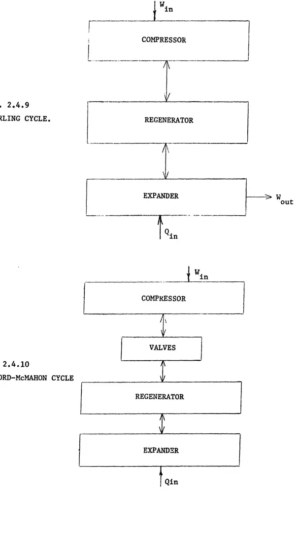
Reversible Refrigeration Cycles: (a) Ericcson; (b) Stirling
Vapour Compression Cycle . . . .. J-T Cycle (a) Schematic (b) T-S Diagram . . . .. Schematic of Ejector Cycle . . . .. Cascade Cycle for Helium Liquefaction . . . . Schematic of an Ideal Gas Cycle . . . .. Schematic of the Claude Cycle . . . .. Stirling Cycle . . . . ) Gifford-McMahon Cycle . . . . I VM Cycle . . . ..
Solvay
Cycle
...
. ...
...
.22
...
25
... ...38 ... ... 42 .43 .....
. 44 .. ee. . . .46 . . 47 . . . . .48 ... .. 50 ... ... 52 ... ... 54 ... ... 54 ... ... 56...
56
3.1 Reversible Continuum Model (a) Mass Crossflow; (b) Variable High Pressure 3.2 Typical Performance Curve for Mass Crossflow Model: Mass Flow Rate
3.3 Cold End Performance Curves for Mass Crossflow Model . . . . 3.4 Cold End Performance Curves For Mass Crossflow Model: . . . .
Fixed Pressure Ratio . . . . 3.5 Specific Heat Capacity Curve for Helium . . . .
3.6 (a) Performance Curves for Mass Crossflow Model: Liquefaction Mode . . 3.6 (b) Cold End Performance Curves for Mass Crossflow Liquefaction Model 3.7 PerformanceiCurve for Variable Pressure Model (Constant) Low Pressure .
3.8 Typical Performance Curve for Variable Pressure Model . . . . 3.9 Mass Recirculation Configuration . . . .. . ...
. . . 18 1.2 1.3 2.1 2.4.1 2.4.2 2.4.3 2.4.4 2.4.5 2.4.6 2.4.7 2.4.8 2.4.9 2.4.1( 2.4.11 2.4.12 . 61 . 63 . 64 .65 .68 . 69 . 70 . 74 . 75 · 79
3.10 Simplified Cold Fnd Configurition (S\'C) . . . 80
3.11 2-Expander Collin's Precooler with Optimail Cold End Conlfiguration . . . . 82
4.1 Typical Precooling
Stage of a Helium Refirigeration
Cycle . .
. . . 86
4.2 Model for Precooling Stage: Heat Exchange with Continuous Expansion . . . 87
4.3 Performance Curves for Ideal Gas Model, Refrigeration Mode. (a) Mass Flow Rate Verslus Temperature . . . 92
(b) Heat Exchange Area . . .. . . 93
(c) Generated Entropy ... .... 94
4.4 Performance Curves for Ideal Gas Model: RefrigeratiQn Mode (Fixed r,) . . 95
(a) Mass Flow Rate . . . 95
(b) Heat Exchange Area . . . 96
(c) Generated Entropy . . . 97
4.5 Performance Curves for Ideal Gas Model: Liquefaction Mode ... 100
(a) Mass Flow Rate . . . 100
(b) Heat Exchange Area . . . ... ... 101
(c) Generated Entropy ... 102
4.6 Cold End Performance Curves for Real Gas, Refrigeration Mode . . . . .. 104
4.7 Performance Curves for Continuous Precooling, Refrigeration Mode . . . . (Heat Exchange Area) . . . 105
4.8 Performance Curves for Continuous Precooling, Refrigeration Mode . . . . (Generated Entropy) . . . 106
4.9 Cold End Performance Curves for Real Gas Model, Refrigeration Mode . 107 4.10 (a) Performance Curves for Mass Crossflow Model: Liquefaction Mode . . 110
4.10 (b) Cold End Performance Curves for Mass Crossflow Liquefaction Model . 111
4.11
3-Expander
Saturated
Vapour
Compression
Cycle
... 115
4.12
Performance
Curves
for
Optimal
3-Expander
Cycle
. ... ... 118
5.2.1 Displacer-Piston Rod Connection Showing Engine Seals
5.2.2 Cylinder Mounting . . . . 5.2.3 (a) Valve Block .. . . . .. . . . . 5.2.3 (b) View of Valve Block . . . .
5.2.4 (a) Overall Layout of Piston Motion Control System 5.2.4 (b) Schematic of Piston Motion Control System .
5.2.5 Hydraulic Controller . . . .
5.2.6 Layout
of Limit Switch
Arrangement . . . .
5.2.7 Cutoff Switch . . . . 5.2.8 NOT Element . . . . 5.2.9 Directional Valve ... 138 ... ...140 ... ...141
...
... . .. .
142
...
144
... ... 145 ... .... 146 ... ... 148...
150
...
150
... ... 151 5.3 Layout of Experimental Set-up: Determination of Refrigeration Capacity . 1575.4.1 T-S Diagram for Defining Wet Expander Efficiency . . . .. 160
5.4.2
Layout
of
Experimental
Set-up:
Static
Heat
Test
... 163
5.4.3 Phase Relationship between Pressure at The Discharge Valve Actuator . . . .
and Inlet Valve Actuator . . . ... 165 5.4.4 Phase Relationship between Pressure in the Expander . . . .
and at the Discharge Valve Actuator . . . ... 166 5.4.5 Phase Relationship between Pressure in the Expander . . . .
and at the Inlet Valve Actuator . . . ... 167
5.4.6 Phase Relationship between Pressure at the Inlet Valve Actuator . . . .
and Displacement (Cylinder Volume) . . . ... 168
5.4.7 Phase Relationship between Pressure at the Discharge Valve Actuator . . . . .
and Displacement (Cylinder Volume). . . . .. 169 5.4.8 Ideal P-V Diagram for Expander . . . 172
5.4.9 Ideal P-V Diagram for Single Phase Expander Mode, with Blow Down . . 173 5.4.10 Ideal P-V Diagram for Single Phase Expander without Blowdown . . .. 175
El.1 Typical Cold End Calibration Curve for Allen-Bradley Resistor . . . 271 E1.2 Full Range Calibration Curve for Allen-Bradley Resistor . . . ... 272
E1.4 (a) Calibration Curves for Vapor Pressure Thermnometer . . . 275
LIST OF SYM'.1BOLS
A Area
Cp Specific Heat Capacity
CF Cost Function
CHX Cost of Heat Exchanger CLN2 Cost of LN2
CPI Consumer Price Index
F Helmholtz Free Energy
M Mass Flow Rate
NTU Number of Transfer Units
AP Pressure Drop Q Heat Transfer T Temperature AT Temperature Difference rp Pressure Ratio S Entropy U Internal Energy V Volume v Specific Volume W Work Transfer
GREEK SYMBOLS
P Dimensionless Constant ln p
77 Efficiency also Dimensionless Temperature
iQ' Dimensionless Mass Flow Rate Ratio n l
A Availability Function
r Specific Heat Ratio ,
Dimensionless Constant R x Dimensionless Constant1+ y 1JT
Joule-Thomson
Coefficient
SUBSCRIPTS c, Constant Volume ex Expander gen GeneratedI Low Pressure Stream
h High Pressure Stream
liq Liquid
n Normalizing Constant
o Initial Volume
I'LA',ES
1A Exposed Engine with control mechanism . . . 131
1B Exposed Engine with vacuum jacket in the background . . . 132
1C Close-up of Engine . . . ... 133
ID Anotherclose-lup view of the Engine ... 134
1E Piston motion control mechanism ... 135
C(hapter 1
IN'''ROI)U('TION
Tlhis chapter gives a brief history of cryogenic refrigecration and states the
purpose of this thesis.
1.1. Intro(duction
Heliunm is classified as a rare gas. It is also perhaps the most difficult gas to liquefy. Yet liquid helium has been the object of more experimemtal and theoretical research than any other fluid except, possibly, water. There are two principal reasons for this unusual attention. First, liquid helium exhibits several peculiar properties suci as superfluidity' 2 which offer challenging scientific investigation. These properties also
have potential applications that can be far-reaching. Secondly, it is an indispensable refi-igerant- for very low temperature work, close to absolute zero temperature. This application puts a high premium on liquid helium. Consequently, there has been a fascinating historical interest in the quest to liquefy helium.3--6 Currently efficient and reliable methods of producing the liquid is of prime interest because the world is on the verge of commercializing superconducting processes and devices.7
Helium was first liquefied by Kamerlingh Onnes in the physical laboratory of the University of Lciden which he had established in 1895. However, this was the culmina-tion of a series of successes in the liquefacculmina-tion of the other cryogenic fluids, in particular, and advances in cryogenic technology, in general, starting with the liquefaction of air in 1877. Therefore the history of helium liquefaction is complete only in the context of the broader history of cryogenic refrigeration. This broader history is outlined in the next section.
a more Mwidly alccepted dfinition. Nilorecover, it is a nattlral dixiding line sinlce ordi-nar) refrigerants like Freoin and hydrogen sulphide boil above this tempelrature whereas the 'permanent'gases - heliuni,hy)drogen.neon,oxygetn etc halle normial boiling points below 123K.
1.2 Ilistory of(ryogenic Refrigeration3 G-10
Any gas may be liquefied by cooling to its condensation temperature and then ex-tracting its latent heat of vaporization. However, for the cryogenic fluids, the condensa-tion temperatures are very low (4.2K at 1 atmosphere for helium) and suitable refrigera-tion at such low temperatures, tradirefrigera-tionally, has not been available. Early attempts to liquefy the cryogens therefore involved other processes.
Robert Boyle's work with gases resulted in his famous law which stipulates that the P- V curve for ideal gases be rectangular hyperbolac. While investigating the validity of Boyle's Law, van Marum discovered, at the end of the eighteenth century, that ammonia gas may be liquefied solely by compression to about seven atmospheres without any necessity of lowering its temperature.
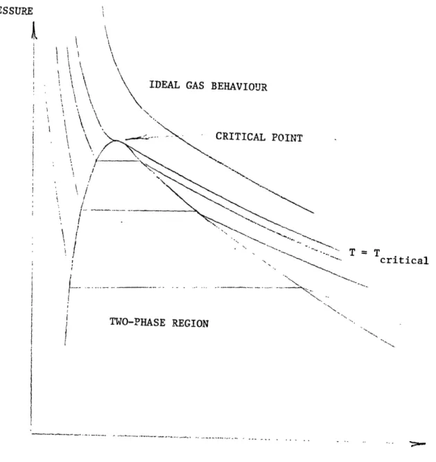
In Michael Faradays's work between 1823 and 1847, he found that both pressure and temperature play a part in the change from gas to liquid. He was able to liquefy several gases by heating one end of a sealed, bent glass tube to increase the pressure of the gas trapped in it and cooling the other end below room temperature. Finally be-tween 1861 and 1869 Thomas Andrews obtained experimental pressure-volume curves for a real gas (carbon dioxide) which showed the characteristic flat portion below the critical point Fig. 1.1. His results illustrate the Pressure-Volume relationship of real gases and indicate that isothermal compression can indeed produce liquid: if the con-stant temperature is below the critical temperature. Consequently, early attempts to liquefy the cryogens involvecd compression of the gases to very hilhl pressures.
PRESSURE ik
I
iI
I
i
=criticalcritical I -- - -- -- - ---- - - - -~- - - -I--~--TWO-PHASE REGION . I. VOLU%EFIG. 1.1 Typical Pressure-Volume
curve for a pure substance. I
These attempts were unsuccessfill because of the low critical point temnperatl.llres of these gases. 'Table 1.1 gives typical values of the critical point parametcers for some cryogens.9
Table 1.1
Critical point parameters for some cryogenic fluids
Fluid Tcriticai (K) Pcritical (atm) Tnorlal bpt. (K)
Oxygen 154.7 50.1 90.19
Nitrogen 126.1 33.49 77.395
n-Hydrogen 33.2 12.98 20.39
Helium 5.2 2.26 4.216
However, it was an effort in this direction which led Louis Cailletet, a French mining engineer to observe that expansion produces cooling when his experimental ap-paratus sprang a leak and the compressed gas escaped into the atmosphere. Subsequently he precooled high pressure oxygen gas in a strong-walled glass tube, released the pres-sure by opening a valve on the apparatus and thereby produced liquid oxygen droplets on December 2,1877.
This was the first time ever a so-called 'permanent'gas had been liquefied. Coincidentally Raoul Pictet, a Swiss physicist, also succeeded in liquefying oxygen on December 22,1877 by a completely different method now called the cascade method. This coin-cidence is interesting for three reasons. First, there was the initial historical confusion over who first liquefied oxygen which was justly resolved in favor of Cailletet. Secondly the different professions of the two men is representative of the two sources of con-tributions to cryogenic refrigeration research: Cailletet typifies the industrial world and Raoul Pictet the research scientist in an institutional laboratory. Thirdly the two processes used have been developed into the two practical liquefaction methods in use today-the methcd of Cailletet has been developed into well-engineered industrial cryogenic liquefaction plants: the method of Pictet has been developed into the cascade
scheime used for tile la!orator) liquefliction of cryogcns. I !.N pl~ants also use a vlariation or the cascade method.
'1The liquid produced by Cailletet in 1877 was in the frmn of mist ethich soon
evaporated. Wroblewski and Olsze% ski were Polish scientists investigating the physical properties of liquefied gases at the Cracow University Laboratory in the samle decade. The were therefore interested in bulk quantities of liquids and introduced two tech-niques to achieve this for air. First the) pumped on the refrigerant used for precooling the gas to fiurther reduce tilhe lowest temperature. Then they developed the a apor shield-ing concept to minimize heat leaks fiom ambient to the test apparatus thereby enhanc-ing prolonged storage of the liquid. Their design consisted of a series of concentric tubes, closed at one end, surrounding the experimental test tube. The cold vapor rising from the liquid flowed through the annular spaces between the tubes intercepting some of the heat travelling toward the cold test tube. Armed with this improvement not only did they succeed in obtaining liquid oxygen in bulk quantities in April 1883, they were also successful in producing liquid nitrogen for the first time a few days later. However their attempts to liquefy hydrogen always resulted in droplets of the liquid: the heat leak to their test apparatus was still large. It thus remained for James Dewar to intro-duce innovations in insulation techniques and subsequently succeed in producing liquid hydrogen in bulk quantities and even go further to produce solid hydrogen.
James Dewar made three particularly significant contributions. He introduced both vacuum insulation, which drastically minimizes heat loss through convection, and the idea of changing the emissivity of radiating surfaces to reduce radiation losses. His device was a double-walled glass vessel with a silvered inner surface. These develop-ments enabled him to liquefy hydrogen in bulk quantities in 1898. However, they were not enough to enable him to produce solid hydrogen until he further cut down on the radiation heat loss by another innovation: the radiation shielding technique. His
produce solid
h)
drogen by pumping the vapor ofil he liquid.11lc success of Cailletet in producing liquid b expansion of a precooled high pres-sure gas led to pioneering efforts in the industrial application of air iquefalction in three centers. In Germany, Linde established the Linde Company for air separation and by 1897 had developed a practical cycle for liquefing air in bulk quantities. Essentially Linde precooled the high pessure gas using a set of counterflow heat exchangers (Fig. 1.2) and throttled the high pressure gas using a Jule lompson valve. (It is surpris-ing that although Joule and Thompson had experimented %with the J-T valve process much earlier, it was Cailletet's observation that actually led to the application of the throttling process in cryogenic refrigeration). In Britain, W. Hampson independently used the same cycle (Fig.1.2) for air liquefaction and actually filed a patent for his device in England two weeks before Linde filed his in Germany. The cycle has since become known as the Linde-Hampson cycle. Meanwhile, in France, Georges Claude was developing a work-producing expansion engine to expand the high pressure gas and thus provide refrigeration by extracting work from the gas. By 1902 he had developed an air liquefaction system using an expansion engine.
The use of expansion engines in air refrigeration'0 dates back to 1849 when a
Florida physician, John Gorrie published a report about his ice making deavice for cool-ing hospitals. It is even claimed that the British Engineer Richard Trevithick built several successful engines ,also for ice making, much earlier although no description of his device was ever published. Charles Siemens incorporated modifications to the Gorrie system involving heat exchangers to obtain a space cooling device in England. The credit for setting forth the essentials of the space cooling refrigerator using air expansion engines however goes to William Thompsom (Lord Kelvin). In any case it is the sys-tematic and persistent effort of George Claude to overcome technical difficulties such as heat leaks and lubrication which led to the successful application of expansion machines in cryogenic liquefaction plants. Consequently he is often cited for introducing the use of cryogenic expansion engines. By 1907 the Claude air liquefier was producing neon as
W. in
V
COMPRESSOR / Rr__
E.~~ ?:
Ii _ C__ _ -+ :---- - I I I1 ,.. EGENEATIVE HEAT EXCHAINGER. LIQUID RESERVOIR Fresh air I intake. I J-T VALV 1 <i I\
J/ I I _ ! I I I I I--I -4" I Ia by product.
'The Linde-Hampson cycle fr air liquefaitction as well as the Claude sstemn had been refined by 1902. Effective insulation protocols had been stablished . I.iquid h3drogen had been produced in large quLiantities and Dewar had even produced solid hydrogen. ilie stage was thus set for the liquefaction of helium which was seen as the gateway towards the march to absolute 7ero. he principal investigators actively engaged in this effort were Olszewski . James Dewar, Morris Travers and Kamerlingh Onnes. They had all tried to use Cailletet's method to liquefy helium and had filed. It was clear therefore that a Linde-Hampson type cycle was required. Kalmerlingh Onnes had an advantage over the other investigators . He had methodically prepared for this onslaught by training skilled technicians. He founded a school for instrument makers and glassblowers in the Leiden laboratory. He built a large liquefaction plant for oxygen, nitrogen and air and followed it up with a hydrogen plant capable of producing four liters of liquid an hour, in 1906. Finally, by June 1908 work on building the helium liquefier had been completed and a high purity gas obtained. On July 10, 1908 he liquefied helium. This indeed was the climax of developments in the preceding thirty years. However, the success is also a tribute to his skill and careful planning especially considering the human resources involved in the operation and the complexity of the cascade machinery for helium.
Although Claude had established the use of work-producing expansion engines for air liquefaction as far back as 1902, it was not until 1934 that the first successfuil attempt was made to liquefy helium by the Claude process, by Kapitza. However, it was the monumental contribution of Sam Collins in 1946 which revolutionalized low tempera-ture research to the extent that the period before 1946 is now referred to as BC (Before
Collins) in cryogenic circles.
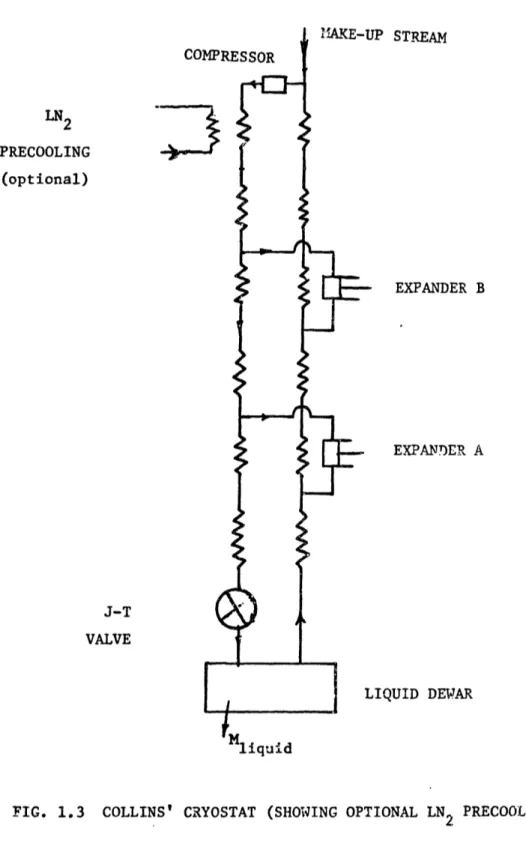
Collins built a practical, dependable helium liquefier using expansion engines which made helium available to most low temperature research centers. The design of the
Collins cryostat (Fig.l.3) w'as based on a second l;iw anallsis. BH considering the flow of entropy in the cycle, he estimated the mass flow to be extracted and fId thlrough the expansion engines. He 'as thereby able to derive a configuration for the liquefier which constitutes an efficient c cle. lie design and fhbrication of the cryostat also incorporated solme ingenious features," whiclh made the cryostat reliable. n'e original cryostat used a Hampson-type heat exchanger but Collins later developed a compact and effective
heat exchanger, called the Joy Tube . Thus te Collins contribution is significant for
t,o reasons: the design was based on sound thernodynanic analysis demionstrating
a clear insight into entropy flow, and the facility used well-designed, well-engineered
components.
Improvements on this system have come fiom two directions. The cycle allows the
flexibility of choosing the temperature levels (expander inlet or discharge temperatures to optimize the cycle performance). Therefore cycle optimization techniques have been
developed and continually improved upon, to select these temperatures. Also efficient
and reliable components have been and are still being developed. This research is a
continuation of work in both directions.
1.3 Applications
Kamerlingh Onnes and his co-workers who first liquefied helium were interested in
investigating the properties of materials at low temperatures and in checking the validity of known natural principles at cryogenic temperatures. Such investigation has led to a catalogue of unique cryogenic phenomena which have prompted several application
ideas. Perhaps the most promising of these potential applications relate to
suiperconduc-tivity. There are two fundamental but related characteristics that underscore the
LN2 PRECOOLING (optional) J-T VALVE
4.
?P STREAM EXPANDER B EXPAND)ER A IQUID DEWARFIG. 1.3 COLLINS' CRYOSTAT (SHOWING OPTIONAL LN PRECOOLING)
extrcmely steady magnetic fields. Some of' the potential pplicatiols arising fiomll these characteristics are discussed presently.
ELECTRICAL GENERA TORS:'2 ' The basic superconducting generator con-cept has been demonstrated and advanced concon-cept designs are being developed
Without the po'er losses associated with resistance heating, superconducting generators consume about to-third less energy than conventional generators with an equixalent power outpult: because of the high current density of the superconductors, the siper-conducting generator is only about two-thirds the size of a conventional genleraltor, is lighter, and can generate higher voltages that conceivably could eliminate the use of step-up transformers in the power supply system. The superconducting generator is more resistant to short-lived line disturbances such as lightning because of its high fields. ELECTRICAL ENERGY STORAGE: 7 This promises to be an efficient means of storing, in the form of magnetic energy, excess electrical energy produced by the utility companies. The utility companies can stockpile the excess electricity generated cheaply at night and use it to meet peak daytime demands. Currently the high daytime demands are handled by expensive oil or gas-fired plants.
ELECTRICAL POWER TRANSMISSION:'" - 22 The use of superconducting cables
for power transmission dramatically increases the current carrying capacity of cables of the same size.
TRANSPORTATION:23 24 The use of superconducting magnets in the magneti-cally levitated train has been demonstrated, with the Japanese National Railways setting a world rail speed record in 1979 of 321 miles per hour with their experimental train. Superconducting magnets are mounted on the train and normally conducting magnets used as guideways. Levitation is provided by induced magnetic fields in the guideway magnets which repel the magnets on the train. Rapidly alternating magnetic fields from
was succCessfill)y tested b3 tile U.S. Naval Ship 1R&) Center in late 1980.
PURKIFICATION /SEPARATION PROCESSES: 23 The difference in magnetic sus-ceptibility of arious materials is tilhe basis of several piurification/spalratio, prcesses.
Tlhus a superconducting magnetic separator may be used to separate iron-containing components from low grade ore or in mining other hard-to-get minerals. In water purification, solids left after sewage treatments are first coagulated uIsually using alum. Magnetic particles are then added to the water and adhere to the coagulated solids. A strong magnet may subsequenltly be used to remove the solid particles. In fact, super-conducting magnets can be used to replace conventional magnets in most separation processes.
NMR MEDICAL IMAGING SYSTEM:2 5- 26 The use of superconductors in NMR medical imaging systems may well be the first commercial application of superconduc-tivity. The performance of NMR imaging systems is greatly enhanced by the use of superconductors because the associated magnetic fields are strong, spatially uniform and very steady. The use of superconductors result in image resolution of 1.3mm compared to 4mm when conventional magnets are used. Also contrasts up to 100:1 versus 32:1 and data collection time of 0.1s compared to 100s indicate the superior images that can be obtained with superconducting NMR. Capital cost of the superconducting NMR may be high but the operating cost will be low because of the minimal power consumption
rate.
FUSION/HIGH ENERGY PHYSICS:2 8 The high fields of superconducting mag-nets make them attractive in replacing conventional magmag-nets in high energy physics experiments and in plasma heating for fusion devices. Also the small size makes them attractive, especially in aerospace applications where relatively small mass is of prime importance . Applications in the bio-medical/chemical field include control of chemi-cal reactions (magnetocatalyses);and suspension/steering of magnetic objects such as the steering of magnetic catheters throu;'- the brain. Superconducting gyroscopes with
extremely small drift are also being developed.
CRYOPUMPING: This is used to create ultra high vacuum for space siulaition tests, for high va\Ctlllnl thermlal ilsLlation and for creating orking cnvironnllelnts in the semiconductor manu facturing industry.
ELECTRONIC DEVICES:2 9-3 0Several sulperconducting electronic devices are being developed. In addition to the low power dissipation, the performance characteristics of various solid state devices at cryogenic temperatures are stable, repeatable and insen-sitive to thermal cycling. These devices have wide applications such as in microwave receivers and as computer elements.
SQUIDS:3 '- 32 Superconducting Quantum Interference Devices reportedly are su-perior to all other magnetic sensors in sensitivity, frequency response, range and linearity. They can therefore perform unique functions not offered by conventional devices. But, in addition. they. can also do less demanding jobs better than conventional instru-ments and are used in highly sensitive magnetometers, gradiometers, and amplifiers-particularly for applications requiring extreme voltage sensitivity.
There is a wide variety of potential applications for superconducting technology. This reflects on the demand for a wide range of refrigeration requirements from large plants, as for the superconducting generator program, to low values of refrigeration (fraction of watts) for cooling superconducting electronic devices. The
commercializa-tion of these and other cryogenic phenomena is contingent upon the availability of
reliable and inexpensive refrigeration plants. The design of rcfiigeration devices there-fore present challenging opportunities for technological innovations to the cryogenic engineer.
1.3.1 Cryogenic Refrigeration at tle N11'T 'ryogenic 'ngineering L,ah)oratory
The monumental contribution of Professor Saim Collins in the forties was the basis for the organization of the MIT Cryogenic Engineering Laboratory where Professor Collins continued to improve helium liquefaction equipment until 1964. After Professor Smith succeeded Professor Collins in 1964, improvement in helium liquefaction were continued and a more efficient liquefier which uses a supercritical wet expander in place of the J-T valve was installed. Refrigeration research was also broadened and several other methods of refrigeration were installed. Prominent among these are the analyti-cal studies and extensive experimental work on Stirling cycle machines, 3 4. thermal
regenerators 35- 4 pulse tube refrigeration 4' and miniature refrigerators 42 using bellows
engine. Contributions from this work have greatly enhanced our understanding of these systems, essentially redefining the basic theory of operation and providing appropriate methods for analyzing these systems. More recently, and especially since the energy crisis the focus of studies in cryogenic refrigeration by Prof. Smith has shifted to a fun-damnental study of the basic refrigeration process. This effort started with a comparative analysis of Collins-type liquefiers operating at elevated pressure levels43 and also marked
the entry of the author into cryogenic refrigeration and the MIT Cryogenic Engineering
Laboratory. Current cryogenic refrigeration work in the laboratory includes magnetic refrigeration studies. It must be mentioned, however, that the laboratory has been at the forefront of other areas of cryogenic technology. The major work in the laboratory involves the superconducting generator. Since testing the world's first superconduct-ing generator with a rotatsuperconduct-ing cryostat in 196912 the laboratory has tested a 3mVA su-perconducting generator' and is currently involved in demonstrating advanced design
1.3.2 Problem Statemenl
Our preliminary study of the perfornmance of hliunl liquefaction cycles operating at
elevated pressure levels indicated a superior performance over conventional cycles. The analysis used the conventional optimization scheme for the Collins-type liquefaction systems. In this conventional technique, a particular cycle configuration is first chosen. A system of equations with the state points (pressure and temperature) and the mass flow rates as the variables is obtained by applying the first law of thermodynamics to various components of the plant and also writing the continuity (mass conservation) equation at the various nodes of the flow schematic. The number of equations (n) is
normally less than the number of variables (m) so that there is an infinite number of solutions to the system of equations, involving m-n arbitrary parameters. Consequently
the system may be optimized by a straight forward mathematical parametric optimiza-tion technique. The resulting soluoptimiza-tion is then checked for violaoptimiza-tions of the second law of thermodynamics. An improvement on this technique by Toscano et al 44 incorporates
the second law by computing the entropy generation associated with each component thereby identifying and quantifying the sources of irreversibilities in the cycle. Our preliminary analysis also used the second law of thermodynamics to judiciously initialize
some of the optimizable parameters' 5.
However, the short comings of this technique was soon apparent. The straight forward mathematical parametric optimization does not provide adequate insight into
the physical factors driving the system. An even more limiting handicap is the fact
that a cycle configuration had to be chosen first. In our analysis we thought of a number of cycle configurations and applied the procedure above to each one of them
in turn. Although we had arrived at a more efficient cycle configuration in the form of the saturated vapor compression cycle, in the end there was no guarantee that we
essentially based on a first law analysis.
These shortcomings of the conventional analysis are the basis for the final objective of this thesis: to develop an alternative design algorithm for cryogenic liquefaction cycles which is based on the second law and, in which the cycle configuration is an
output rather than an input.
Our preliminary analysis had shown that the saturated vapor compression cycle is
superior, in thermodynamic performnnance, to the conventional cycle. When used for the
production of atmospheric pressure liquid helium, it allows the cycle pressures to be chosen independently of the liquid dewar pressure and thus allows these pressures to be
selected for the best performance of the expanders and heat exchangers in the cycle and
hence better overall performance.
For refrigeration at temperatures below 4.2K, the wet expander cold-compressor
section is used to maintain subatmospheric pressure over the boiling liquid and thus allows the conversion of a standard helium liquefier to a 1.8K refrigerator without the
addition of large low pressure heat exchangers and large displacement vacuum pumps. An approximate cost estimate also indicated that a saturated vapor compressor is worth
developing. In view of these superior characteristics, the second objective of this thesis
is to investigate, experimentally, the feasibility of implementing the saturated vapor compression.
Thus the objectives of this research are:
1. To develop an alternative optimization scheme for cryogenic liquefaction cycles, based on the second law of thermodynamics and in which the configuration is an
output rather than an input.
2. To design and build a machine that can be used for investigations leading to the
The thesis stalls in chapter two with a discussion on the choice of entropy flow as
the method of analysis and the generated entropy as the performance index, followed
by a brief review of mechanical cryogenic refrigerators. In chapter three, reversible continuum models for the precooling stage of a typical refrigeration cycle are considered for synthesizing an optimum cycle configuration using the basic theory of chapter two. The new entropy flow optimization technique for designing helium liquefaction cycles is presented in chapter four. An account of the experimental work involving the design and fabrication of a reciprocating machine with a programmable hydraulic-pneumatic control and the evaluation of its performance is given in chapter five. Finally chapter six summarizes the salient points of the research.
ChapIer 2
'11
II.XlO)X NAMICNIN('
F 1111(I.R.!'
lON
C'Y1NE'I!!S
'('LS.
Tllis chapter discusses the tuse of entropy flow, analysis in cr. ogenic
refriigeration and tilhe choice of generated entropy as the perfor-mantce index for the analyses in sbsequent chapters. A brief review of several mechanical refiigerators is also given.
2.1 Introduction
Refrigeration processes are essentially heat transfer processes. Invariably all prac-tical heat transfer processes are accompanied by irreversibilities. Therefore since the keyword in this thesis is thermodynamic performance, it is important to quantify the irreversibilities in a way that lends itself to analytical optimization.
In this chapter, the generated entropy concept of the second law of thermodynamics40 is shown to be an invaluable tool for quantifying the concept of thermodynamic irre-versibility as well as efficiently identifying the origin and/or location of the irrevers-ibilities (section 2.2.1). The cycle generated entropy is next shown to be equivalent to the coefficient of performance COP as a cycle performance index (section 2.2.2). Then a general requirement for refrigeration cycles is discussed which further underscores the role of entropy in refrigeration processes (section 2.3). Finally, examples of mechanical refrigeration cycles are presented in section 2.4 to contextualize the SVC cycle which is the main concern of this thesis.
2.2.1 iEntropy Flom Analysis
The first law of thermod3ynamics defines energy as a propertn) of a system and gives the interrelationship between the change ill energy of a systeli and the energy transfer interactions associated with the system and its environment. Also the second law
intro-duces entropy as a property. It is the entropy transfer which distinguishes between heat and work transfer interactions as parallel forms of energy transfer for a thernod)ynarmic simple-system. It is onl) the transfer of energy as heat which is accompanied by entropy transfer. Further the second law directly imposes limits on the heat transfer between a system and its environment. Combining the first and second laws then reveals the
limits imposed on the work transfer interaction. To illustrate, consider a closed system experiencing an isothermal change of state from initial state (1) to a final state (2). The first law gives the energy relationship:
Q-.2- W1-2 = U2- U1. (2.1)
The second law gives Cte limit on the heat transfer
Q1.-2 < T,(S2- ), (2.2)
or alternatively
Q1-2 + ToS,. = T(S2-
S1).
(2.2))The generated entropy, s,,. is a path dependent variable. The difference between pos-sible paths is described by the strength of the inequality sign in Eq. (2.2a) or by the magnitude of s,,,n in Eq. (2.2b). For a reversible path, the equality holds in Eq. (2.2a) and S,,en = o. Thus, Sg,,, gives a quantitative description of the degree of irreversibility of the process, which is missing in the inequality statement.
or
WI .*2 + 7TS,,.,I, = - -
F]
(2.A)w1Chere y is thile [Cllllt.Z free energy and ';, is required to specify the final location on the thermal scale of the entropy generated b the irrevcrsibilit. By imposing tile ,additional restriction that the environment is at constant pressure, P,, the limit on the isothermal non-pdv work is givcln by the Gibbs free-energy:
(wVI .2),,o,, ,,,,. < - [(u + F:,v- T,,S), - (U + P,,V -- T,,S),]. (2..z)
The limit on the heat transfer is still given directly by the second law in Eq. (2.2). Further, ifthe environment is assumed to be the atmosphere, the maximum useful work available for the system atmosphere combination is given by the availability function A :7
(WI -2)u/efu, = A2 - A, (2.-a)
where
A = (U + PtrnV - T,,,S)- (U + PatmV - Tt,,,,S)minimum. (2.')
Similarly for an open system experiencing heat transfer only with a heat reservoir at
T.,,,,, again the second law directly imposes a limit on the heat transfer interaction:
Q
<
E
mTt..-
mtmS(2.
)out in
or
Qv
+ TatmSen = E ,Tt,. s- mT",MS. (2.,)out in
To determine the limit imposed on the shear work transfer combine the first and second laws to get
(
fi alua:a--
r
m(h -- 7 )--Z n(h - S) (2. a)Io il ()
where
4: (h- T,,,,S) ,-- ( - 7,t,,,,S),. (2.8)
Thus the maximum useful *work obtainable is given by the change in the availability function, (also called excrgy). Exergy is a relative quantity defined with reference to a dead state, usually the atmosphere.
In summary then, for refrigeration cycles the principal energy interaction of interest is heat transfer. Associated with this heat transfer is entropy transfer. Refrigeration cycles essentially absorb heat from some low temperature T, and reject this heat at some higher temperature. Equivalently refrigeration cycles absorb entropy at and move this entropy through a temperature gradient and reject it at some higher temperature. In the process of moving the entropy, irreversibilities occur at various temperature levels which are quantitatively given by the generated entropy. The entropy generated adds on to the entropy being moved through the temperature gradient. Thus there is a cascading effect. The total entropy eventually rejected at the hot end (or at any temperature level for that
matter) indicates the degree of irreversibility of the cycle. Thus the path of the cycle dctennines the total value of non-property s,,, which indicates the degree of departure
of the cycle from reversibility.
The entropy flow analysis is therefore the natural mode of analysis for such refrigera-tion cycles. Further for cryogenic refrigerarefrigera-tion cycles several heat reservoirs may be used at different temperature levels such as in the cascade process. Heat may be rejected at
excr!Iy analy)sis. Finally, tilhe entropy flow alnal)sis Ilnables tile cnlrop neratcd locally (and hence the irreversibilities) to be monitored thus facilitating conti InIuI analysis.
Entropy flow analysis is therefore invaluable in the design of efficient refrigeration cycles which requlires mininlizing irrcversibilitics generated over the the nlperattlre range
of interest as discussed presently.
2.2.2 (eneraltel Entropy as 'erfornlance Index
Cryogenic liqucfaction/refrigeration cycles may be optimized based on several criteria such as maximum refrigeration (liquid extraction), minimum energy (busbar), minimum plant capital cost, minimum total input power per unit mass circulated or in terms of availability ratios. In general the various criteria do not necessarily result in the same optimum condition and the actual design condition involves trade-offs between some of these criteria. For example, designing for optimum thermlodynamic perfor-mance requires expensive equipment: a reversible heat exchanger should have an in-finite heat exchange area. The basic criterion used in this research is the thermodynamic performance of the cycle as measured by irreversibility. Trade-offs will then be based on the degree to which changes in a particular system parameter affects the thermodynamic performance.
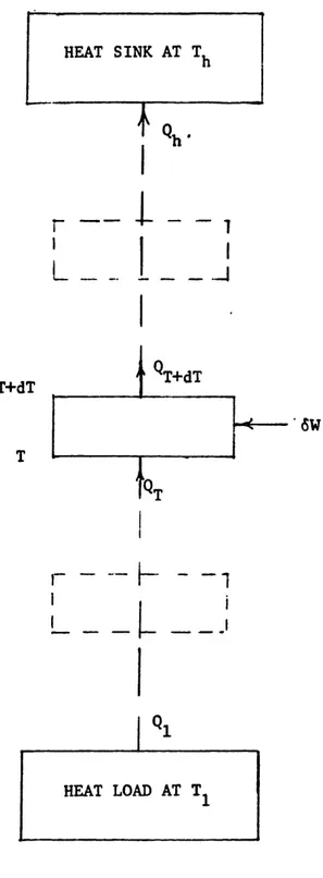
The performance of thermodynamic cycles is traditionally given by an efficiency parameter or the coefficient of performance COP. An entropy flow analysis for evaluat-ing the performance of a refrigeration system composed of a series of refrigerators (Fig. 2.1) is now discussed to establish in a simple case the relation between the generated
entropy performance index and the conventional COP.
The refrigeration system shown in Fig. 2.1 is a cascade of differential refrigerators distributed between T, and T with each refrigerator spanning a temperature dT. The work input for each stage is
I I
rL
I L - -T+dT T _ 1s ~1 -4-QT+dT CSWr --
-I
I i I .IFIG. 2.1 REFRIGERATION SYSTEM COMPOSED OF A SERIES OF REFRIGERATORS.
where 6i4r,, is the reversible work for the differential refrigerator stage.
The overall performance of te refrigeration system is indicated by the COI' which is derived in appendix A by integrating over the temperature splan of the system
coP= (2.10)
W (ThIT,-1 (2.10)
from which the COP for a reversible refrigerator is recovered for z = i
COP,', = 1 (2.11)
Th/T,- (2. The COP can be expressed in terms of entropy by substituting for the temperature ratio. The expression for this substitution is derived by first evaluating the heat transfer at any temperature T,
=Q (. (2.12)
The entropy-temperature relationship is then given by
(=
(T)-l
(2.13)
The temperature ratio in Eq. (2.10) may now be replaced by the entropy ratio in Eq. (2.13) to give
1
COP= (2.14
S~ ( r ) -- 1 Finally substituting for
s = 1+ -,
we can express
Eq. (2.14(2.)
15)
COP=
-
(2.16)
To. 1 + S, -- 1
Therefore maximizing COP is equivalent to mliniizing s.,,,,(7') given by
&,. , ,
= A ---
dT.
(2.17)T, dT
Since s,.,, is the integral over the precooling range of the local irreersibility, this example also illustrates the cascading effect of the irreversibilities associated with the refrigeration process.
The analyses in the next two chapters involve differential elements of a continuum model for the precooling stage of the refiigeration cycle. The local irreversibility given by dSe,, is integrated to determine the total irreversibility which is subsequently
mini-mized. The equivalence established here between the COP and the generated entropy illustrates the use of the integrated entropy as a perfornmance index.
2.3 General Requirement for Refrigeration
In order to further underscore the importance of the entropy flow concept in the analysis of refrigeration cycles, the dependence of refrigeration effect on the entropy changes associated with changes in a generalized variable of the refrigeration system is discussed in this section.
In the analysis of the common refrigeration cycles, the thermodynamic simple-system model is adequate for determining the cycle performance. Thus in applying the first law, only forces arising from the pressure have been taken into account in calculat-ing the reversible work f Pdv. The effects of body forces due to external force fields are
choosing the intensive variables as indclcindent ariables, til entropy changc is given by
dS =
(a'-
dT+
(- pT
(2.18)The refrigeration (Q) provided by the mechlanical refrigeration systerm at a given con-stant temperature levei T. is thus given by
6Q < TdS
<
T,(OS
dp (2.19)Thus the refrigeration effect depends on entropy changes associated with changes in the intensive mechanical work variable. This may be generalized to other refrigera-tion modes by relaxing the restricrefrigera-tions on the external force fields imposed on ther-modynamnic simple-systcms.4 8
50 The reversible work transfer may then be due to some
other conservative force such as magnetic forces. (The change in magnetic field strength associated with magnetic work transfer is the basis of refrigeration by adiabatic demag-netization.) Thus a fundamental prerequisite for any refrigeration method is that there must be an identifiable property whose changes cause changes in entropy at constant
temperature.
Magnetic refrigeration51- 54 is primarily used for providing refrigeration below 4K
in a single cycle mode. Magnetic refrigerators that provide conltinuous refrigeration are not yet well developed. By far the most widely used cryocoolers/refrigerators use mechanical cooling effect. This research deals with the efficient design of these mechanical cooling devices. The underlying principles of various types of mechanical refrigerators are discussed presently.
2.4 N.leclianicali Refrigeration (ycles
2.4.1 Reversible Refrigeration Cycles
Typically, mechanical refrigeration cycles are fluid flow systems that absorb heat Q at the refrigeration temperature T. and reject heat A, at a higher temperature T,,. For
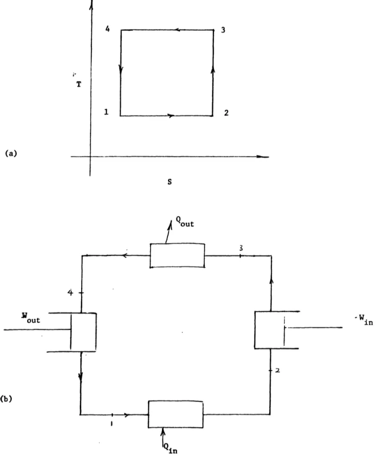
such two-heat reservoir cycles to be reversible, the entropy transferred at T (associated with the refrigeration effect) is transported, unchanged. against the tenmiperatuLre gradient, and rejected at T,,. Figures 2.4.1(a) and 2.4.2 show typical T-S diagrams for some revers-ible refrigeration cycles.5'- 59 Historically, these cycles were first developed for power cycles and by reversing the direction of executing the cycle, the corresponding refiigera-tion cycle is derived. Consequently the cycles are often qualified by "reversed" as in reversed Carnot cycle.
2.4.2 Vapor Compression Cycle (VCC)
In the reversed Carnot cycle, the isotherms are joined by constant entropy processes 2-3 and 4-1. The arrangement of components in Fig. 2.4.1(b) can conceptually be used to effect this steady flow cycle if all component steady flow processes are reversible. This is the basis of the ideal vapor compression refrigeration cycle.59 60 The working fluid is usually freon, ammonia, or hydrogen sulphide.
In the Carnot VCC, the refrigeration is provided by the latent heat of vaporization of the refrigerant. The expansion engine thus must operate in the two-phase region. This causes practical problems that degrade the performance of the engine. Therefore an expansion valve is routinely used for the expansion process. The valve also has the advantage of simplicity.
T (a) ( 4 1 3 2 S
FIG. 2.4.1 REVERSED CARNOT CYCLE: (a) T-S DIAGRAM
-w.
in
V j
-I K 1 S (a) T a
constant
1 S (b) I - - -T AJ--4 J-T valve i I
kin
...
.
T0 boundary ----Ti~in
F, II r' 1 (a) IQ in / / 3 , (b) SFIG. 2.4.3 VAPOUR COMPRESSION CYCLE : (a) SCHEMATIC
(b) T-S DIAGRAM
.L
_I_ _·__I___ ________ 1___ _______·_C_____ · --- -·---ilr
I I II -.---- i z_ T i~ T ! i 'r _
the critical temperature of tlh rfi'rigerant is greater th;an the ambient tlpclrature. This cycle is therefore commonly used for air-conditioning applications close to room tenm-peralture. Secondly, the cycle high temperature is less than the critical templeratilre of the
working fluid so that the state of the working fluid is liquid after the heat rjection stage. This cycle is therefore used ~with non-cryogelic rfirigerants.
2.4.3 Joule-Thompson Cycle
The Joule-Thompson cycle Fig. 2.4.4 is the analogous vapor compression scheme for gases with critical point temperatures far below ambient temperatures', 62. Unlike the
conventional vapor compression cycle this uses regenerative heat exchange to precool the high pressure gas before throttling. The T-S diagram for a typical Joule-Thompson cycle is shown in Fig. 2.4.4(b) and indicates a closer resemblance to the Ericsson rather than the Carnot cycle.
To understand what makes this cycle work, consider first the cold box Fig. 2.4.4 The temperature To is the boundary between the cold box and the hot end. In general the temperature T is less than T by the heat exchange AT. Therefore much of the compressor work input is above T and in the limiting case of reversible heat exchange there is no work input below T. In this case the first law of thermodynamics applied to the cold box gives:
Q = - m(h,p - p)To. (2.20)
Thus the enthalpy difference at the To boundary accounts for the refrigeration Q. In general the enthalpy change is due to a pressure effect as well as a temperature effect:
Qout 1 TO BOUNDARY ___~~~~~~~ 0._ ~~~~~~~~~~~~~~~~~~~~~~~~~~~~~~~~ t X -1 5 >
?
' 2-4 3 (a) i _ ~~~~~~~~~~~~~~- -i I~~~~~~~~~~~~~ 1 I, T at TL3 STAGE COMPRESSION UNIT
5
S
(b)
FIG. 2.4.4 J-T CYCLE: (a)SCHEMATIC; (b) T-S DIAGRAM
i 6
t--- Wi in--
'.W
in
1 2 TL - .- --- ·--- --- ·I·---··--·-··----· ·---L---) CF-
--- - 1
... __ _where -(ah = CP (2 22)
\(BPj,)=
CT
(2.23)
(9O(h \=
AP'
NtdP~)TY
t)h ~(2.24) = --j Cp (2.25)Since qc, o, the heat exchange AT has a negative effect on the refrigeration poten-tially available diminishing it by mC,,AT. If j, > o then the Up effect is positive and this is responsible for any refrigeration produced. Thus it is the non-ideality at To that makes the cycle work since p, # o. The temperature T must lie below the Joule-Thompson inversion curve (,j, > o).
Joule-Thompson cycle refrigerators have been miniaturized with correspondingly low cool down times of the order of seconds.6 3 These miniature J-T refrigerators (few
millimeters diameter, few centimeters long) often use bottled high-pressure gas and are well-suited for cooling small electronic devices: they have negligible vibrational/magnetic noise since there are no moving mechanical parts. By incorporating an ejector into the
cold end of the J-T cycle, lower temperatures may be reached.
Refiigeration with working fliuds which have low inversion temperatures uses a modified Joule-Thompson cycle, the cascade method, in which fluids with decreasing critical point temperatures are successively used to provide precooling Fig. 2.4.6. Nitrogen and hydrogen are used in succession in the liquefaction of helium by this method. This is the method used by Karnerlingh Onnes to liquefy helium in 1908.
HELIUM STAGE W I I i I I ! -I ,ER C > 1 I
FIG. 2.4.6 A CASCADE CYCLE FOR HELIUM LIQUEFACTION. i i i LIQUID HELIUM DEWAR AMMONIA STAGE NITROGEN STAGE HYDROGEN STAGE Q. q W W J-T VALVE X t HEAT EXCHANC J I <1" I 1-, 1-
2.4.4 Ideal Gas Cycle
It is the non-ideality effect of the working fuid, indicated by 4J, > o, which provides the refrigeration in the J-T cycle. Therefore for helium refrigeration at temperatures above say 80 K, where helium approximates ideal gas behaviour, the J-T expansion process cannot be used. In general for an ideal gas cycle, mechanical work-producing-expansion processes are used as in the Carnot cycle configuration of Fig.2.4.1. Usually additional precooling is provided by regenerative heat exchange in counterflow heat exchangers.
There is a dependence of work distribution in the cold box on the fluid properties. For the reversible vapor compression cycle, the cold box requires work input whereas, in contrast, the reversible ideal gas cycle provides a work output. To determine the nature of this dependence, consider the cold box shown in Fig. 2.4.7. The expander work is derived from the first and second laws of thermodynamics and simplifies to
We=mf(To-
(,)
dP+
f
vdP.
(2.26)The entropy term can be substituted from the Maxwell's relation
-= - Lp , (2.27)
and the expander work becomes
We
-{
(T.
T)f(-
dP+
vdiP].
(2.28)
P
Therefore the isobaric coefficient (&v/OT)p (or equivalently (as /P)T) of the working
.--
Win __ T. BOUNDARY ff ._ ___ .__ __.1
i ni
i ! iiI //\
I%/
QlFIG. 2.4.7 SCHEMATIC OF AN IDEAL GAS CYCLE.
______ Qout