Publisher’s version / Version de l'éditeur:
Bulletin of the American Meteorological Society, 2018-02-12
READ THESE TERMS AND CONDITIONS CAREFULLY BEFORE USING THIS WEBSITE.
https://nrc-publications.canada.ca/eng/copyright
Vous avez des questions? Nous pouvons vous aider. Pour communiquer directement avec un auteur, consultez la première page de la revue dans laquelle son article a été publié afin de trouver ses coordonnées. Si vous n’arrivez pas à les repérer, communiquez avec nous à PublicationsArchive-ArchivesPublications@nrc-cnrc.gc.ca.
Questions? Contact the NRC Publications Archive team at
PublicationsArchive-ArchivesPublications@nrc-cnrc.gc.ca. If you wish to email the authors directly, please see the first page of the publication for their contact information.
NRC Publications Archive
Archives des publications du CNRC
This publication could be one of several versions: author’s original, accepted manuscript or the publisher’s version. / La version de cette publication peut être l’une des suivantes : la version prépublication de l’auteur, la version acceptée du manuscrit ou la version de l’éditeur.
For the publisher’s version, please access the DOI link below./ Pour consulter la version de l’éditeur, utilisez le lien DOI ci-dessous.
https://doi.org/10.1175/BAMS-D-16-0047.1
Access and use of this website and the material on it are subject to the Terms and Conditions set forth at WIVERN: a new satellite concept to provide global in-cloud winds, precipitation and cloud properties.
Illingworth, A. J.; Battaglia, A.; Bradford, J.; Forsythe, M.; Joe, P.; Kollias, P.; Lean, K.; Lori, M.; Mahfouf, J.-F.; Mello, S.; Midthassel, R.; Munro, Y.; Nicol, J.; Potthast, R.; Rennie, M.; Stein, T. H. M.; Tanelli, S.; Tridon, F.; Walden, C. J.; Wolde, M.
https://publications-cnrc.canada.ca/fra/droits
L’accès à ce site Web et l’utilisation de son contenu sont assujettis aux conditions présentées dans le site LISEZ CES CONDITIONS ATTENTIVEMENT AVANT D’UTILISER CE SITE WEB.
NRC Publications Record / Notice d'Archives des publications de CNRC: https://nrc-publications.canada.ca/eng/view/object/?id=a10cbafb-a84a-400a-a781-8b5ec0789f5d https://publications-cnrc.canada.ca/fra/voir/objet/?id=a10cbafb-a84a-400a-a781-8b5ec0789f5d
Bulletin of the American Meteorological Society
EARLY ONLINE RELEASE
This is a preliminary PDF of the author-produced
manuscript that has been peer-reviewed and
accepted for publication. Since it is being posted
so soon after acceptance, it has not yet been
copyedited, formatted, or processed by AMS
Publications. This preliminary version of the
manuscript may be downloaded, distributed, and
cited, but please be aware that there will be visual
differences and possibly some content differences
between this version and the final published version.
The DOI for this manuscript is doi: 10.1175/BAMS-D-16-0047.1
The final published version of this manuscript will replace the
preliminary version at the above DOI once it is available.
If you would like to cite this EOR in a separate work, please use the following full citation:
Illingworth, A., A. Battaglia, J. Bradford, M. Forsythe, P. Joe, P. Kollias, K. Lean, M. Lori, J. Mahfouf, S. Mello, R. Midthassel, Y. Munro, J. Nicol, R. Potthast, M. Rennie, T. Stein, S. Tanelli, F. Tridon, C. Walden, and M. Wolde, 2018: WIVERN:
AMERICAN
METEOROLOGICAL
SOCIETY
A new satellite concept to provide global in-cloud winds, precipitation and cloud properties. Bull. Amer. Meteor. Soc. doi:10.1175/BAMS-D-16-0047.1, in press.
WIVERN: A new satellite concept to provide global in-cloud winds,
1
precipitation and cloud properties.
2
3
A.J. Illingworth*1, A. Battaglia2, J. Bradford3, M. Forsythe4, P. Joe5, P. Kollias6, K. Lean7, M. 4
Lori8, J-F Mahfouf9, S. Mello5, R Midthassel10, Y. Munro11, J. Nicol1, R. Potthast1,12, M.
5
Rennie7, T.H.M. Stein1, S. Tanelli13, F. Tridon2, C.J. Walden3, M.Wolde14. 6
7
Affiliations: 8
1 Department of Meteorology, University of Reading, UK
9
2University of Leicester, Leicester, & National Centre for Earth Observation, UK.
10
3Science and Technology Facilities Council, UK
11
4Met Office, UK
12
5Environment and Climate Change Canada (ECCC), Canada
13
6Stony Brook University, Stony Brook, NY, USA
14
7European Centre for Medium-Range Weather Forecasts, Reading, UK
15
8HPS-GmbH Munich, Germany
16
9MétéoFrance, France.
17
10European Space Agency, European Space Research and Technology Centre, NL
18
11Airbus Defence and Space Limited, UK
19
12Deutscher Wetterdienst, Germany
20
13Jet Propulsion Laboratory, California Institute of Technology, USA
21
14National Research Council, Canada
22
23
24
Manuscript (non-LaTeX) Click here to download Manuscript (non-LaTeX) double-space-text-figs-16-Dec-2017.docx
* Corresponding author address: Anthony J. Illingworth, Department of Meteorology, 25
University of Reading, Earley Gate, PO Box 243, Reading RG6 6BB, UK. 26 Tel: +44 118 378 6508 27 E-mail: a.j.illingworth@reading.ac.uk 28 29
ABSTRACT 30
This paper presents a conically scanning space-borne Dopplerized 94GHz radar Earth 31
Science mission concept, WIVERN, ‘Wind VElocity Radar Nephoscope’. WIVERN aims to 32
provide global measurements of in-cloud winds using the Doppler shifted radar returns from 33
hydrometeors. The conically scanning radar could provide wind data with daily revisits 34
poleward of 50°, 50-km horizontal resolution and approximately 1km vertical resolution. The 35
measured winds, when assimilated into weather forecasts and provided they are 36
representative of the larger scale mean flow, should lead to further improvements in the 37
accuracy and effectiveness of forecasts of severe weather and better focusing of activities to 38
limit damage and loss of life. It should also be possible to characterize the more variable 39
winds associated with local convection. Polarization diversity would be used to enable high 40
wind speeds to be unambiguously observed; analysis indicates that artifacts associated with 41
polarization diversity are rare and can be identified. Winds should be measurable down to 1 42
km above the ocean surface and 2 km over land. The potential impact of the WIVERN winds 43
on reducing forecast errors is estimated by comparison with the known positive impact of 44
cloud motion and aircraft winds. The main thrust of WIVERN is observing in-cloud winds, 45
but WIVERN should also provide global estimates of ice water content, cloud cover and 46
vertical distribution continuing the data series started by CloudSat with the conical scan 47
giving increased coverage. As with CloudSat, estimates of rainfall and snowfall rates should 48
be possible. These non-wind products may also have a positive impact when assimilated into 49 weather forecasts. 50 51 52 CAPSULE (20-30 words) 53
A new satellite concept with a conically scanning W-band Doppler radar to provide in-cloud 54
winds, together with estimates of global rainfall, snowfall and cloud properties. 55
56
According to the World Meteorological Organization (WMO), wind-storms are by far the 57
largest contributor to economic losses caused by weather related hazards, resulting in 58
approximately 500 billion USD (adjusted to 2011) of damage over the last decade globally 59
(Zhang 2016). With more than 50% of the Earth’s population concentrated in coastal 60
developments and mega-cities, extreme weather events have an increasing potential to cause 61
significant and recurring damage in terms of both loss of life and economic loss. As such, 62
Disaster Risk Reduction has been singled out by the WMO as their number one strategic 63
priority, highlighting the importance of improving the accuracy and effectiveness of forecasts 64
and early warnings of high-impact meteorological environmental hazards (Zhang 2016). 65
Baker et al. (2014) provide an excellent review of the need for global wind measurements and 66
argue that the measurement of the three-dimensional global wind field is the final frontier that 67
must be crossed to significantly improve the initial conditions for numerical weather 68
forecasts, and quote WMO as determining that global wind profiles are “essential for 69
operational weather forecasting on all scales and at all latitudes”. Assimilation of additional 70
wind observations from the 94 GHz radar on the proposed future WIVERN satellite into 71
weather forecast models should significantly improve weather prediction skill allowing better 72
focus of mitigation activities with respect to timing, location and assigning resources. 73
74
Particularly striking examples of the advantages of mitigation activities are the tropical storm 75
“Nargis” that hit Myanmar in 2008, when no preventive action was taken and 138,000 died, 76
and the subsequent more powerful storm “Phaillin” that struck the E Coast of India in 77
October 2013 but caused only 43 fatalities because timely warnings were issued, and a mass 78
evacuation of those living in the coastal regions was organized. In Europe, the windstorms in 79
1999 were estimated to have caused €18.5B of damage, and in 2009 on 24 January the very 80
deep depression ‘Klaus’ caused 28 deaths through drowning as it crossed the coast of western 81
France leaving 1.7 million people without electricity. A succession of rapidly deepening 82
depressions forming over the western Atlantic crossed the UK during December 2015 and 83
January 2016 with the heavy rain and flooding resulting in insurance losses of about €1.5B. 84
85
WMO has outlined the systematic observation requirements for satellite-based products 86
(GCOS 2006) as part of their Rolling Requirements Review process and also maintains 87
requirements in the Observing Systems Capabilities Analysis and Review tool (OSCAR 88
2016). The relevant numerical weather prediction (NWP) requirements for winds are 89
summarized in Table 1. One conically-scanning WIVERN radar placed in Low Earth Orbit 90
could measure the line-of-sight (LOS) component of the horizontal wind and should be able 91
to satisfy the breakthrough requirements in Table 1 for in-cloud winds, except for the 6-hour 92
observing cycle that would require multiple satellites. To achieve the observation 93
requirements of having a fine vertical resolution and a short observing cycle, we currently 94
envisage (Table 2) a 94 GHz (3.2 mm wavelength) radar with a 2.9 by 1.8 m elliptical 95
antenna producing a narrow, conically scanning pencil beam at 38° nadir and 41° off-96
zenith at the surface with an orbit altitude of 500 km and a surface footprint of approximately 97
1 km in diameter. These parameters are chosen as a compromise between the need to have a 98
higher orbit and thus a broader ground track to reduce the satellite revisit time, and the 99
consequent requirement of a much larger antenna to maintain the 1 km vertical resolution 100
when the slant path to the surface is increased. The 2.9 m elliptical antenna would have a 101
beamwidth of 0.11° in the horizontal and 0.08° in the vertical, so, in combination with a 3.3 102
μs pulse length (500 m round-trip slant path), the vertical resolution (-3 dB) would be about 103
800 m assuming both the antenna beam pattern and pulse shape are Gaussian. 94 GHz is the 104
preferred frequency as a 35 GHz radar would have a pencil beam 2.7 times wider with 105
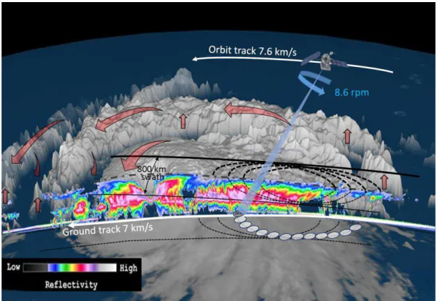
consequent loss of vertical resolution. As indicated by the sketch in Fig. 1, the antenna would 106
rotate once every 7.5 seconds tracing out a circular ground track 800 km in diameter 107
advancing 50 km for each revolution. 108
109
The WIVERN mission will be complementary to other observing systems providing unique 110
insights into the structure of winds within clouds and precipitating systems. The impact on 111
Numerical Weather Prediction (NWP) is expected to be on features in the models that are 112
long-lasting when compared to the revisit times, so it will be necessary to identify convective 113
motions that are not representative of the large-scale flow. The Aeolus Doppler wind Lidar 114
satellite mission (Stoffelen et al. 2005) is expected to measure line-of-sight winds in clear air, 115
through optically thin clouds/aerosol and from the top of optically thick clouds/aerosol, but it 116
lacks the penetrating capability of a radar for measuring within most clouds. To improve 117
NWP forecasts the need is for wind observations upstream of the areas were the wind damage 118
may occur 24 to 48 hours later; McNally (2002) has shown that these ‘meteorologically 119
sensitive areas’ are often cloudy. Fig. 2 shows the coverage expected in one day for the 120
notional WIVERN configuration of a 500nkm orbit tracing out an 800 km diameter ground 121
track that results in a revisit time of about once a day for latitudes poleward of 50° and more 122
frequent visits over the polar regions. These regions have become an important area for 123
climate and weather studies as demonstrated by the recently launched WMO “Polar 124
Prediction Project” that aims to promote cooperative international research enabling 125
development of improved weather and environmental prediction services for the polar 126
regions. In the Arctic the fast warming, the decrease in ice cover and the recent opening of 127
the Northwest Passage have attracted attention. The limited number of ground based profiling 128
observations in the Arctic regions indicate the ubiquitous presence of light precipitation often 129
limited to the lowest 4 km whose properties may be sensitive to the local and mid-latitude 130
aerosol transported from mid-latitudes. WIVERN observations would provide pan-Arctic 131
coverage and reveal the true physical and dynamic characteristics of the clouds and 132
precipitation in these data sparse regions. 133
134
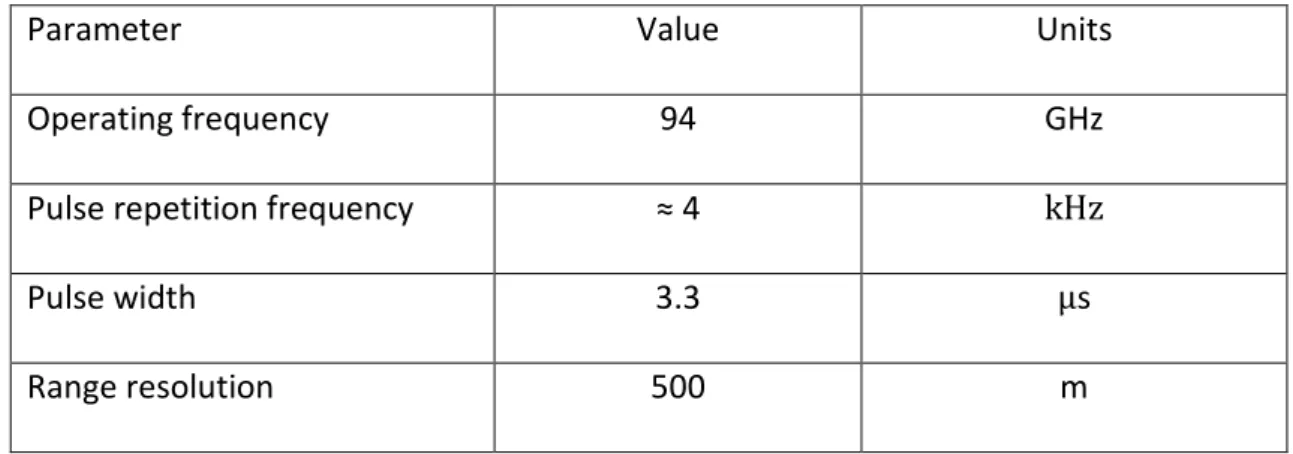
THE WIVERN CONCEPT AND PREDICTED DOPPLER PERFORMANCE. 135
WIVERN would utilize a 94 GHz transmitter similar to the one that has been operating 136
beyond expectations on the nadir-pointing CloudSat Cloud Profiling Radar (Stephens et al. 137
2008, Tanelli et al. 2008) since its launch in 2006. CloudSat transmits 3.3 μs (500 m) pulses 138
at a pulse repetition frequency (PRF) of approximately 4 kHz with 1800 W peak power (at 139
beginning of life) and 24 W mean radiated power. By integrating the pulses for 0.16 s, 140
equivalent to a distance of 1.09 km along track, during which about 600 pulses are 141
transmitted, it was therefore possible during CloudSat’s prime mission to detect targets with 142
reflectivities above -30 dBZ and a single pulse signal-to-noise ratio (SNR) of 0 dB for an 143
echo of ≈ -16 dBZ. The proven performance of CloudSat can be used both to estimate the 144
accuracy of the retrieved LOS speeds from WIVERN, and the climatology of radar 145
reflectivity profiles around the globe from several years of CloudSat data can be used to 146
predict the number of occasions that WIVERN would observe accurate winds. An 147
improvement in the sensitivity of WIVERN compared to CloudSat can be expected, because 148
of the shorter slant path to the ground (≈ 650 km vs CloudSat’s ≈ 710 km) and the larger 149
antenna (1.8 m by 2.9 m for WIVERN vs CloudSat’s circular 1.8 m). This should lead to a 150
single pulse SNR of 0 dB for a return of ≈ -19 dBZ, and for integration lengths of 1, 5 and 10 151
km the reflectivity threshold for 0dB SNR will be -24dBZ, -27.5dBZ and -30.5dBZ, 152
respectively. 153
154
The EarthCARE satellite (Illingworth et al. 2015) will use the conventional pulse pair 155
technique to detect the nadir Doppler velocity of the hydrometeors, using a PRF of 7.5 kHz, 156
so that only one pulse at a time is present in the troposphere, but this leads to a folding 157
velocity of just 6m s-1 and a noisy Doppler estimate because of the low correlation of the
158
phases of the pulse pair echoes. As explained in the sidebar, ‘Why polarization diversity’, 159
WIVERN overcomes this dilemma by estimating the Doppler velocity using the polarization-160
diversity pulse-pair (PDPP) technique (Pazmany et al. 1999) and will transmit a pair of pulses 161
one with horizontal polarization (H) the other with vertical (V), with a short separation, Thv.
162
A value of 20 μs is proposed for Thv so that the folding velocity is 40 m s-1 and large enough
163
to comfortably exceed the errors of the winds calculated in the NWP models. The pulse 164
separation would be 3 km along the slant path or 2.3 km in the vertical. 165
166
WIVERN would trace out a quasi-circular ground track of diameter 800 km on the ground, 167
advancing 50 km along track for each rotation with the footprint traveling at 335 km s-1 or 1
168
km in 3 ms. If it were to use the same 4 kHz PRF as CloudSat, in each km it could transmit 169
10 H-V pulse pairs each with a 20 μs separation to measure Doppler, interleaved with 2 170
single H or V pulses to measure the LDR of the targets to flag any potential problems of cross 171
talk between the two polarizations. The ten pulse pairs would alternate between H-V and V-H 172
to distinguish between phase shifts due to Doppler and to differential phase shift on 173
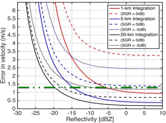
backscatter (Pazmany et al. 1999). The predicted Doppler accuracies for 1, 5 and 20 km 174
integrations are displayed in Fig. 3. The measured sight component (LOS) of the wind can be 175
converted to the horizontal line-of sight winds (HLOS) winds if the vertical wind component 176
is assumed to be zero. To satisfy the WMO requirement of a horizontal wind component 177
(HLOS) of 2 m s-1 an LOS wind accuracy of 1.35 m s-1 is needed, this can be achieved for 20 178
km integration if the echoes are > -20 dBZ, and for 5 km they should be above -15 dBZ, 179
provided there are no ghosts caused by cross talk between H and V returns. Note that factors 180
such as beam pointing knowledge and non-uniform beam filling (discussed later) may well 181
prevent the theoretical accuracies < 0.5 m s-1 being achieved for the higher dBZ values. 182
183
To gauge the number of sufficiently accurate wind observations expected from the proposed 184
WIVERN satellite and their susceptibility to ghosts, an analysis of reflectivity profiles 185
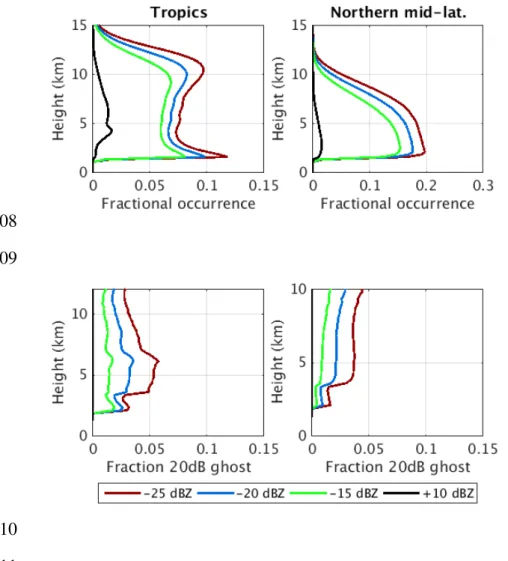
averaged over a 20 km along track integration for four years of CloudSat data is displayed in 186
Fig. 4. The upper panel shows that, averaged over the tropics and northern mid-latitudes, 187
clouds with echoes > -20dBZ are present for about 10% of the time between heights of 1 and 188
10 km, and this fraction does not change markedly for reflectivity thresholds of 25, 20 and -189
15 dBZ. These figures are for 20 km integration but change by less than 0.2% for shorter 190
integrations down to 1 km. For clouds 10 km deep, the sloping WIVERN sample at cloud top 191
will be displaced by 7 km horizontally compared to the ground footprint, the insensitivity of 192
the CloudSat statistics to the integration length suggests that this horizontal displacement and 193
areas of broken cloud will not bias the WIVERN observations. The vertical resolution of 194
WIVERN winds should be better than 1km, so, for a 20 km integration and before thinning, 195
on average one wind with an accuracy better than 2 m s-1 (HLOS) should be detected every 196
60 ms or 1.4 million per day. 197
198
‘Ghost’ echoes caused by cross-talk between the H and V returns may occur when there are 199
high reflectivity depolarizing targets 2 km above or below much weaker targets. The phases 200
of the ghost echo are uncorrelated with the true return signal so their effect will be to increase 201
the random error in the velocity estimate at each gate; this may occur over several 202
neighbouring gates but these random errors should not introduce any bias as the ghost echoes 203
decorrelate between successive pulse pairs. The lower panel in Fig. 4 is a plot of CloudSat 204
observations for each height level, ‘h’, of the fraction of the time that there is a denser cloud 205
with a reflectivity 20 dB greater at a height either 2 km above or below ‘h’. For clouds with 206
reflectivities above -15 dBZ this occurs about 2% of the time. As a worst case we assume that 207
the LDR of the denser clouds is -15 dB, then on 2% of occasions there would signal-to-ghost 208
ratio (SGR) of -5 dB; Fig. 3 shows that the LOS velocity accuracy of 1.35 m s-1 could still be 209
achieved for 20 km integration for dBZ > -10dBZ. We conclude that significant ghost echoes 210
from hydrometeor returns should be rare. In the next section we will present some 211
observations to support this conclusion. We will also consider the more serious problem of 212
ghost echoes and biases in the velocity estimates in gates close to the surface as a result of 213
surface clutter, and the biases due to both the vertical wind shear and by the satellite motion 214
when there is non-uniform beam filling. 215
216
If the winds from WIVERN are to be assimilated it will be necessary to identify regions 217
where LOS winds are affected by convection and are not a representative component of the 218
large-scale horizontal wind. Anderson et al. (2005) have analyzed aircraft observations of 219
tropical convection and define an updraft core as a region of diameter > 500 m having a 220
vertical velocity > 1 m s-1 and find that 90% of such cores have diameters of less than 3 km in 221
diameter. One year’s continuous observations of profiles of vertical velocity and reflectivity 222
made with the zenith-pointing 35 GHz cloud radar at Chilbolton, UK, confirm that regions of 223
up and down drafts exceeding 1 m s-1 are absent in stratiform clouds, and confined to 224
convective regions where the reflectivity values exceed +10 dBZ. From Fig. 3 we conclude 225
that the LOS velocity should be accurate to 1.35 m s-1 for each km along the ground track 226
provided Z is above -5 dBZ. We propose that convective regions should be identified by 227
significant changes in LOS velocities on the km scale and flagged as non-representative for 228
global NWP data assimilation users. These fluctuations of the observed LOS velocities 229
should be of interest to those studying the characteristics and statistical properties of 230
convective processes and for validating cloud-resolving models. The detailed evolution of 231
individual convective clouds cannot be observed from a single satellite in low earth orbit so 232
such studies are best conducted from aircaft. 233
234
GCOS has recently recommended (GCOS, 2017) a satellite be launched to continue the data 235
set that CloudSat has been gathering on cloud reflectivity profiles since its launch in 2006 236
and to be continued by EarthCARE. WIVERN should be able to provide such data. Miller 237
and Stephens (2001) show that a minimum detectable signal of -28 dBZ should detect a 238
fraction of the true cloud field sufficient to reconstruct the instantaneous top-of-the 239
atmosphere to within Clouds of the Earth’s Radiant Energy system (CERES) requirements. 240
WIVERN should achieve -27.5 dBZ sensitivity for 5km along ground track integration (50 241
pulse pairs) corresponding to 15 ms integration time; whereas CloudSat and EarthCARE will 242
have a 5km nadir along track reflectivity sample about every 0.8 s suggesting that WIVERN 243
would obtain about a fifty fold increase of IWC profiles. 244
245
The hydrometeor cloud targets are not perfect tracers of the wind, so a correction would be 246
needed to account for their terminal velocity. Battaglia and Kollias (2015) reported that the 247
error in the mean terminal velocity of ice clouds is a function of their reflectivity and is < 0.2 248
m s-1 up to 10 dBZ and that the random error for Z < -5 dBZ is 0.5 m s-1; this should 249
introduce a random error of < 1 m s-1 into the inferred horizontal component of the wind.
250
For rainfall at 94 GHz Mie scattering by the larger raindrops leads to a Doppler velocity of 251
about 4 ± 1 m s-1 (Lhermitte 1990) so a correction accurate to < 1m s-1 of the HLOS winds 252
should be achievable. When the radar gate straddles the melting layer, the terminal velocity 253
changes rapidly, but such occasions can be flagged by the high values of the depolarization 254
ratio, LDR, resulting from the irregular rocking motion of the wet oblate melting snowflakes. 255
256
POTENTIAL SPURIOUS SIGNALS FROM THE DOPPLER RADAR. 257
Ground clutter. Surface clutter contamination can affect the hydrometeor Doppler signal; if 258
the signal to clutter ratio (SCR) is 15 dB it will lead to a 3% bias of the hydrometeor velocity 259
towards the surface zero velocity. The shape of the clutter signal is determined by the 260
combined effect of the WIVERN antenna pattern, its pulse-shape, and the illumination 261
geometry while its intensity is driven by the surface backscattering properties (Meneghini and 262
Kozu 1990). A recent aircraft campaign funded by ESA and conducted in Canada using the 263
NRC Airborne W-band radar has characterized the surface return at WIVERN incidence 264
angles (410) both for ocean and flat land surfaces (full details in Battaglia et al. 2017). Over
265
ocean the normalized backscattering cross sections () are over 30 dB smaller than at nadir 266
with typical values of -25 dB but roughly ranging between -35 dB and -15 dB with larger 267
(smaller) values in presence of strong (weak) wind and when looking upwind (crosswind). 268
Sea surfaces are moderately depolarizing at such angles with an LDR about -15 dB. Ocean 269
backscattering properties are characterized by a strong angular dependence but land surfaces 270
are more constant with of the order of -10 dB. Forest-covered and rural surfaces present 271
very similar results, whilst urban surfaces generate slightly higher values of . 272
273
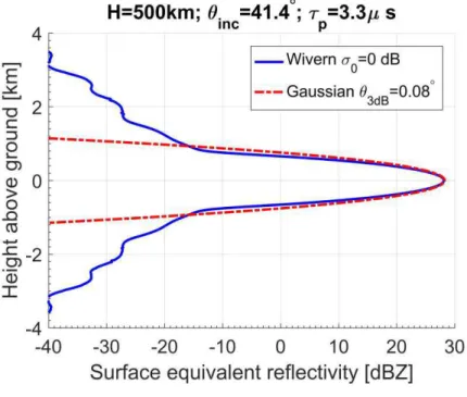
The clutter expected for a WIVERN configuration when observing a flat surface with 0
274
dB is illustrated in Fig 5a for the WIVERN antenna pattern which was derived in the ESA-275
DORA ITT study (inset of Fig. 5b). The first antenna sidelobe at 0.150 is 20 dB below the
276
maximum are clearly affecting the surface clutter above 1 km altitude. Clutter signals scale 277
with and are therefore expected to be about 10 dB (25 dB) lower than those depicted in 278
Fig. 5a over flat land (the ocean). If snow-covered surfaces have lower than 0 dB (still to 279
be determined by observations) the plot in Fig. 5a suggests that it will be possible to produce 280
snow retrievals similar to CloudSat, with clutter contamination only in the last km close to 281
the surface for Zsnow > -10 dBZ, and at lower altitudes for higher reflectivities. LOS winds
282
must be derived only in regions with large signal-to-clutter ratios (15 dB or above). For 283
reflectivities 3dB above the minimum detection threshold this means that the surface signal 284
must be lower than -30 dBZ. For characteristic values of sea and land this seems to be 285
achievable at heights above 1 and 2 km, respectively 286
287
Cross polarization interference and the effect of “ghost” echoes. The ability of the 288
polarization diversity scheme to derive wind velocities relies on limiting the coupling 289
between the polarizations both at the hardware level typically reducing values to < -25 dB, 290
while the wave propagates and scatters in the atmosphere. At the WIVERN incidence angles, 291
atmospheric targets like melting hydrometeors and columnar crystals can produce LDR up to 292
-12 dB (Wolde and Vali 2001) whilst surface clutter tends to depolarize more over land (LDR 293
values of -9±3 dB) than over sea (characteristic value of -15 dB, Battaglia et al. 2017). The 294
effect of cross-polarization is to produce an interference signal in each co-polar channel 295
depending on the temporal shift between the H and V pair and the strength of the cross-polar 296
power (which is given by the product of the LDR and the co-polar power) and appear as 297
``ghost echoes’’ (Battaglia et al. 2013). The phases of ghost echoes are incoherent with 298
respect to the echoes of interest so do not bias the velocity estimates, but increase their 299
random error as a function of the signal to ghost ratio (SGR) (Pazmany et al. 1999); as 300
illustrated by the dashed lines in Fig. 3 when the SGR falls to 0 and -5 dB this random error 301
increases rapidly for shorter integration lengths. By replacing two in ten of the pulse pairs by 302
a single H or V pulse, the LDR of the targets can be monitored and used to flag occasions 303
when there may be cross talk between the H and V echoes. 304
305
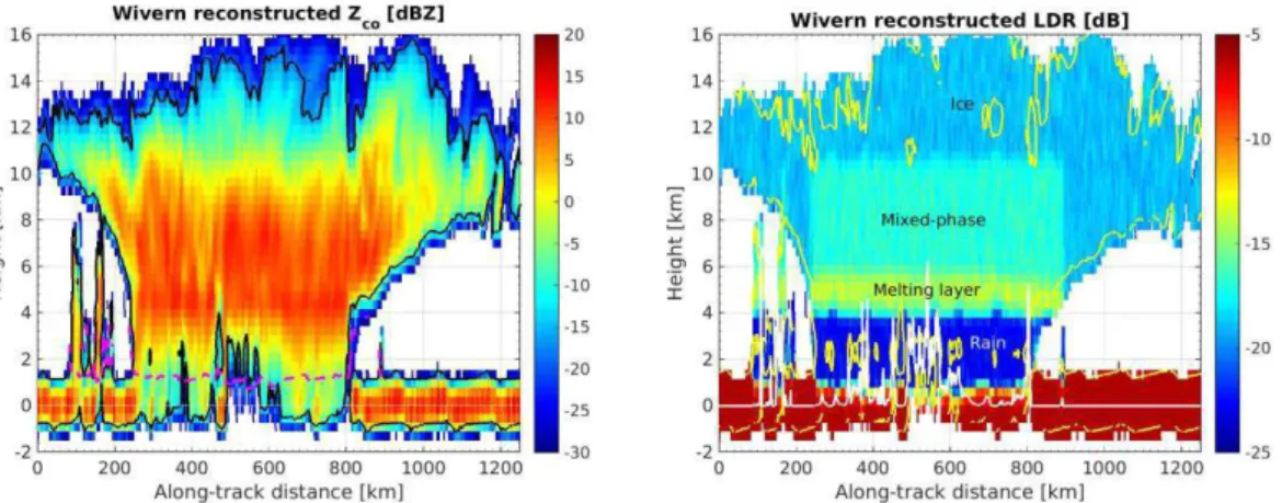
Figure 6 shows simulated WIVERN observations of reflectivity and LDR of a stratiform 306
precipitating system over the Pacific observed on the 10 January 2008 reconstructed by tilting 307
and wrapping the vertical CloudSat curtain so as to be along the WIVERN scanning 308
direction. CloudSat effective reflectivity and attenuation are derived from the 2C-RAIN 309
product. The reconstruction accounts for the WIVERN observation geometry, its antenna 310
pattern and assumes a 5 km integration length. LDR values sampled from normal 311
distributions are used for rain, ice crystals, melting layer particles and mixed-phase clouds, 312
with means of -23, -19 –14 and -17 dB and standard deviations of 2, 1.5, 1.5 and 1.5 dB, 313
respectively. These values have been selected based on a climatology collected at the 314
Chilbolton Observatory. Clutter with the shape shown in Fig. 5a and representative of flat 315
land surfaces, having normally distributed with mean value of -8 dB and standard 316
deviation 4 dB, has been included. The reflectivity (panel a) clearly shows a region of strong 317
attenuation in correspondence to the precipitation core (~2-6 mm h-1) located around 600 km. 318
The black line contours the region where Doppler velocities estimates are expected to have 319
accuracies better than 2 m s-1 when adopting a T
hv equal 20 µs. The SCR is typically >20 dB
320
(magenta line) for heights above 2 km where bias in velocities will be negligible. Ghost 321
echoes (see sidebar 2) are expected when the SGR is < 3dB (yellow line in right panel) and 322
are confined to the high reflectivity gradients at the cloud boundaries (where Doppler will be 323
too noisy anyway) and close to the surface (that would be much reduced over the sea). 324
325
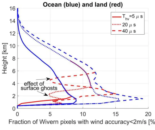
A month of CloudSat data (Jan 2008) have been used to simulate WIVERN profiles and the 326
ghosts generated by Thv values of 5, 20 and 40 μs taking into account the SNR, the SGR, and
the SCR for each 5 km along track integration length in order to assess the fraction of profiles 328
for which WIVERN is expected to produce winds with accuracy better than 2 m s-1 (Fig. 7. 329
The fraction is much lower for the 5 μs Thv values because the increased noise error maps
330
into a large velocity error. Overall Fig. 7 shows that in the mid-troposphere (3-8km) 331
WIVERN would provide a useful measurement 10% of the observation time, but reduced to 332
5% over land at heights near to 2 and 4km where the bright land surfaces produce ghost 333
echoes for Thv of 20 and 40 μs, respectively, indicating that 20 μs may be optimum.
334
335
Ground-based validation of theoretically predicted wind errors and biases. The degree to 336
which ghost echoes and/or vertical gradients in reflectivity combined with vertical wind shear 337
can lead to increased random errors or biases in the wind estimates made from space by 338
WIVERN, can be assessed using recent observations made with the 94 GHz radar at 339
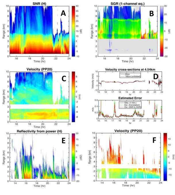
Chilbolton in Southern England pointing 45° off-zenith with a time resolution of six seconds 340
and gate length of 60 m. The case of 27 June 2017 (Fig. 8, panels A to D) is chosen because 341
of the large gradient in received power exceeding 20 dB for the 3 km/20 μs separation of the 342
H-V pulse pair (panel A); this will lead to signal to ghost (SGR) ratios of 0 dB and -5 dB for 343
LDR values of -20 dB and -15 dB (not shown – but in the melting layer at 4 km range they 344
reached -15 dB resulting in the SGR of -5 dB at 7.5 km range). The velocity estimated with 345
Thv = 20 μs (panel C) at a height of 4.54 km where SGR is at its lowest is plotted in black in
346
panel D (upper trace) whereas the ‘true’ velocity from the H-H pulse pairs separated by 160 347
μs (when there will be no ghost echoes) is in red; the increased gate-to-gate random noise 348
introduced by the ghosts in the black trace when SGR is low is very clear when compared to 349
the smooth red trace. The lower trace in panel D shows that the observed increases in the rms 350
error for a Thv = 20 μs agree very well with two independent theoretical predictions of the
351
error (see Fig. 3); one based on the SNR and SGR computed via the LDR estimate, and a 352
second based on the drop in observed correlation between the H-V returns due to the increase 353
in the noise. This plot confirms that ghosts increase the random error of the wind estimate but 354
do not introduce any bias. Ghosts are observed relatively frequently from the ground, because 355
of the ~10 dB change in received power from the same target at a range of 1 km and 3 km. so 356
they are useful for validating the theory, but ghosts should be much less frequent from space, 357
because of the negligible fractional change in range of the targets (see Fig. 4b). Biases in the 358
radar-derived winds may arise when there is a vertical wind shear that coincides with a large 359
vertical gradient of radar reflectivity; this is the case in panels A and C where at a slant range 360
of 4.5 km the reflectivity across the bright band changes by 10 dB in 1 km and the vertical 361
wind shear is about 5 m s-1. These radar observations are taken every six second with a gate
362
length of 60 m. From the average winds at this resolution, the true velocity for a WIVERN 363
sample volume of 800 m length by 10 minutes (equivalent to a horizontal distance of 10km 364
from the satellite if the horizontal advection velocity is 1 km min-1) can be computed and the 365
bias derived by comparing this ‘true’ velocity with the reflectivity weighted mean velocity 366
that would be detected by WIVERN. From this image WIVERN would obtain 550 wind 367
samples with an rms LOS wind error of 0.16 m s-1 and an average bias of 0.07 m s-1, but for 368
data assimilation purposes the data would be thinned. The case above was chosen because of 369
the marked bright band, but panels E and F illustrate the case of 28 Aug 2017 when a region 370
of wind shear of 20 m s-1 per km and reflectivity gradients of up to 20 dB km-1 descended by 371
2-3 km in 10 hours. The biases can also be predicted from changes in velocity from 372
neighboring samples at the WIVERN resolution and the observations rejected when this 373
exceeds 0.3 m s-1. The result is that ~ 20% of the WIVERN samples are rejected, and the
374
remaining WIVERN observations have a bias of 0.05 m s-1 and an rms error of 0.34 m s-1. 375
376
Non-Uniform beam filling (NUBF). For fast-moving space borne Doppler radar, reflectivity 377
gradients within the radar sampling volume can introduce a significant source of error in 378
Doppler velocity estimates (Tanelli et al. 2002). When adopting slant-viewing geometry the 379
situation is illustrated in Fig. 5b, with the shading of the WIVERN sampling volume 380
indicating the strength of the backscattered signal. The red and green arrows indicate the 381
apparent velocity introduced to the WIVERN volume due to the motion of the satellite (green 382
toward and red away from the satellite); as a result, for the case illustrated, a downward bias 383
will be produced. Notional studies have demonstrated that such biases can be mitigated by 384
estimating the along-track reflectivity gradient (Schutgens 2008, Kollias et al. 2014; Sy et al. 385
2014). For WIVERN the relevant gradients are those along the direction in the plane 386
generated by the satellite velocity and by the antenna boresight and is orthogonal to the latter 387
(identified by in Fig. 5b). As a consequence, NUBF effects are linked to reflectivity 388
gradients along different directions depending on the scanning position of the rotating 389
antenna, with NUBF velocity biases expected to be linearly proportional to such reflectivity 390
gradients with a coefficient of the order of 0.1-0.15 m s-1 dB-1 km (Battaglia and Kollias 391
2015). When side-looking, the relevant reflectivity gradients are those along-track, which can 392
be estimated from the reflectivities measured along the scanning track and used to mitigate 393
the NUBF effect. However, such mitigation is increasingly less feasible when moving from 394
side to forward/backward-looking angles where the relevant reflectivity gradients correspond 395
to a direction that is orthogonal to the scanning track. However, thanks to the WIVERN 396
conical scanning geometry, on average, the biases looking in opposite directions with respect 397
to the satellite motion cancel out and NUBF leads only to an increase in the random error of 398
the wind. A high-resolution (0.5 km horizontally and 0.3 km vertically) synthetic reflectivity 399
field obtained from a WRF simulation of hurricane Isabel has been used to estimate the 400
NUBF-induced errors of WIVERN measurements. Preliminary results show that errors 401
should be less than 0.5 m s-1 for side-looking and 2 m s-1 for forward/backward-looking 402
angles. More work is needed in order to properly characterize the variability of the wind and 403
of the 94 GHz reflectivity field at the WIVERN sub-pixel scale. Data sets obtained via 404
airborne of ground-based 94 GHz Doppler radars could be used to test the detrimental NUBF 405
effect on Doppler measurements. 406
407
Pointing Accuracy. The rotating antenna will introduce a sinusoidal component of the 408
satellite velocity with an amplitude of about 5,000 m s-1. If the bias is to be less than 0.5 m s-1 409
then the radar electrical boresight elevation and azimuthal angles should be known to < 100 410
μrad. If the radar is used as an altimeter, the elevation angle can be continually monitored by 411
measuring the range as the antenna scans over the sea; for a slant range of 651 km, an error of 412
100 μrad would manifest itself as an apparent change in range of the sea surface of 42 m. For 413
a point target with an SNR> 20 dB, Skolnik (1981, page 402) shows that changes in the time 414
of the leading edge of the return echo can be estimated to within 5% of the echo rise time; 415
simulations using distributed scatterers on the sea surface confirm that this accuracy can be 416
maintained by averaging 100 pulses (10 km along the ground track). Turning to the 417
requirement to know the azimuthal angle to 100 μrad, equivalent to a distance along the 418
scanning ground track of just 65 m, or about one tenth of the beamwidth, an error of 100 μrad 419
in pointing knowledge will result in a sinusoidal velocity error with maxima of ± 0.5 m s-1 420
when pointing across track. More studies are needed on this topic, but we propose two 421
approaches. Firstly, when pointing precisely across track ground clutter will appear to be 422
stationary and averaging over many scans should identify the precise angle at which this 423
happens, and, secondly, we will use regions of light winds where the ECMWF analysis 424
provides winds accurate to better than 1 m s-1 to make small adjustments to the azimuthal 425
pointing knowledge to remove the systematic biases when pointing across track.. 426
427
Multiple scattering. When dealing with space-borne millimetric radars, in the presence of 428
highly attenuating media, the multiple-scattering signal can overwhelm the single scattering 429
contribution (Battaglia et al. 2010) with very detrimental effects both on retrieval and 430
Doppler products (Battaglia and Kollias 2014). Studies based on CloudSat have demonstrated 431
that multiple scattering is not negligible in the presence of high-density ice (hail and graupel) 432
or moderate/intense rain, (Battaglia et al. 2011). With an LDR mode, segments of the profiles 433
affected by multiple scattering can be easily flagged (e.g. by the condition LDR>-10 dB, see 434
Battaglia et al. 2007) and excluded from further wind analysis. Indeed air motions in these 435
conditions would not be assimilated into the model even if they had been properly retrieved, 436
as they are not representative of the large scale flow and are transient features compared to 437
the revisit time of the satellite. 438
439
440
THE IMPACT OF WIND OBSERVATIONS ON GLOBAL NWP MODELS. 441
The main impact of the WIVERN wind observations should be realized through their 442
assimilation into global NWP models. The ‘Forecasting Sensitivity to Observations’, ‘FSOI’ 443
technique (Langland and Baker 2004), implemented in the ECMWF model by Cardinali 444
(2009), is a very powerful tool that enables, for the first time, quantification of the impact of 445
individual observations that are assimilated in to the NWP forecast model in reducing the 446
“forecast error” obtained by comparing the T+24 forecasts of temperature, wind, humidity 447
and surface pressure with their corresponding analyses. The contributions of the top five 448
observation types in reducing this forecast error for the Met Office, ECMWF and 449
MétéoFrance global models are displayed in Table 3. This shows that both the in-situ aircraft 450
observations and the “Atmospheric Motion Vectors” (AMVs, the winds derived from the 451
movement of cloud or water vapour features in successive satellite images), make an 452
important contribution to reducing forecast errors, second only to the humidity and 453
temperature structure provided by the IR and microwave sounders. 454
455
The initial high resolution AMV wind observations are thinned in the ECMWF global model 456
to provide, at most, a single wind estimate for each 200 by 200 km horizontal ‘box’, a vertical 457
thinning of 50-175 hPa that varies with height, and a 30 minute temporal thinning. This 458
thinning is to account for the spatial and temporal correlation of AMV winds errors over 459
large distances due to errors in the height assignment. The figures for the Met Office are 460
similar: 200 by 200 km, 100 hPa and two hours. ECMWF blacklist AMV winds over land 461
below 500 hPa, while the Met Office is not quite so strict with a height limit over land 462
usually closer to 600 hPa north of 20°N. If observations are assimilated at too high a 463
horizontal density, the fact of not accounting for spatial correlations of observation errors in 464
the analysis can also degrade the resulting forecasts (Liu and Rabier 2002). Aircraft winds do 465
not suffer from problems associated with strong spatial correlations and screening over land, 466
and in the ECMWF model are used for a height range that extends down to within 1 km of 467
the surface and are currently thinned to 70 km in the horizontal and 15 hPa; this will be 468
reduced to 35 km and 7.5 hPa in 2018. Currently, about half of all aircraft winds are below 469
500 hPa. The case studies discussed in Fig. 8 suggest that the radar-derived winds should 470
have similar error characteristics to aircraft winds but may be rather larger because of their 471
800m vertical resolution. 472
473
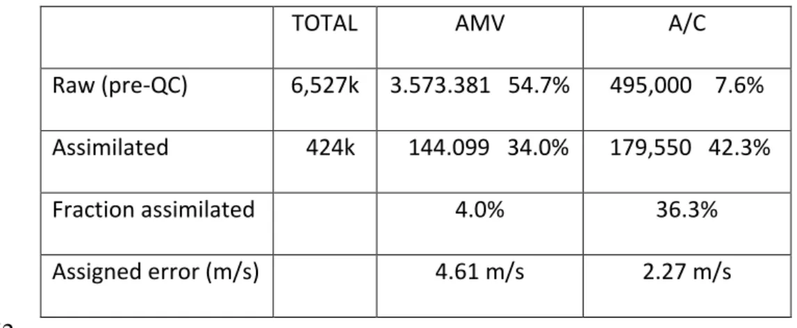
Table 4 compares the contributions of the AMV winds and the in-situ aircraft measurements 474
to the ECMWF global model and shows that when AMV winds are assimilated they are, on 475
average, assigned a random error of 4.6 m s-1 for the zonal component of the wind, but for the 476
in-situ aircraft winds the error is only 2.3 m s-1. Combined with the larger thinning of the 477
AMV winds, the net result is that only 4% of the AMV observations are assimilated as 478
opposed to 36% of the aircraft observations. The CloudSat analysis summarized in Figs. 4 479
and 7 indicatesthat about 1.3 million winds with a resolution of 20 km along track would be 480
obtained each day. If these were thinned to 50 km, similar to the ECMWF value planned for 481
aircraft winds in 2018, then the number assimilated could be about 500,000 per day. By 482
comparison with the figures in Table 4, this suggests that their impact on the forecast should 483
be significant. 484
485
The winds from WIVERN are only line of sight but Horányi et al. (2015a) have demonstrated 486
that, with a state of the art data assimilation system and real observations, HLOS winds such 487
as would be obtained from an aircraft provide about 70% of the impact of a vector wind, and 488
that in the tropics the impact of wind data is much greater than the mass information. 489
McNally (2002) provides further evidence for the potential impact of in-cloud winds. He 490
investigated the sensitivity of the weather forecasts to errors in the analysis of the current 491
atmospheric state that subsequently develop into significant medium-range forecast errors. 492
The main obstacle was the presence of cloud in these ‘sensitive’ areas; depending on the 493
amount and altitude of cloud cover the information from infrared (IR) sounders (advanced or 494
otherwise) could be severely limited. 495
496
If winds are to be assimilated it is extremely important that the systematic errors of the 497
observations are not too large relative to the random errors. Simulations carried out to predict 498
the potential impact of the winds from the Aeolus satellite by Horanyi et al. (2015b) have 499
shown that assimilating winds that are biased by 1-2 m s-1 when the random error standard 500
deviation is around 2 m s-1 will actually degrade the forecast unless the bias can be estimated 501
and removed prior to assimilation. Our analysis suggests that winds from WIVERN should 502
only be biased when they are affected by ground clutter and that such regions should be easy 503
to identify. 504
505
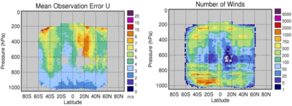
The mean observation error and the number of AMV winds from Meteosat 10 that were 506
assimilated into the Met Office model for the month of December are plotted in Fig. 9. The 507
AMV error is a combination of error in the tracking step and an error in speed due to an 508
uncertainty in the height assignment as discussed by Salonen et al. (2012); Forsythe and 509
Saunders (2008) describe how the assigned AMV velocity error increases with the vertical 510
wind shear in the model. For heights above 500 hPa and for all latitudes, the mean 511
observation error is mostly in the range 5 to 9 m s-1. The maximum number of assimilated 512
winds is found at around 900 hPa over the Southern Oceans, followed by heights of 200-400 513
hPa at all latitudes, with a lower number of winds in mid-levels. The vertical distribution of 514
ECMWF assimilated winds is also bimodal with fewer winds between 400 and 700h Pa. 515
Analysis of CloudSat data (Figs 4and 7) suggests that one advantage of the WIVERN winds 516
should be the absence of the current mid-level gap in coverage. 517
518
The actual numbers of AMV U-component winds assimilated into the ECMWF model during 519
a 12-hour cycle in October 2016 are displayed in Fig 10 for each 10° by 10° area over the 520
globe. The numbers are expressed as the number of observations per 106 km2 area with the 521
data having been thinned to 200 by 200 km ‘boxes’ in the horizontal, so that along the 522
equator, a value of 100, would be equivalent to 4 winds per box in the 12 hour period. When 523
predicting the performance of WIVERN we assume a thinning to 80km, close to the current 524
ECMWF value for aircraft winds, and use the CloudSat data to calculate for every 80 km 525
along-track segment how often there is a cloud echo of at least 5km length where the 526
reflectivity exceeds -18 dBZ, for which (from Fig. 3) we expect the velocity error to be less 527
than 2 m s-1. CloudSat has only a small footprint at nadir, so to simulate the 800km wide 528
circular ground path, we multiply these numbers by 11, and calculate on average the number 529
of winds per 106 km2 area in a 12 hour period as displayed in Fig. 10. This Fig. indicates that 530
the number of WIVERN winds assimilated should be of similar magnitude to the current 531
AMV winds. 532
533
Recent experience at Météo-France has shown that increasing the vertical resolution of 534
observations in the 4D-Var data assimilation system of the global ARPEGE NWP model, has 535
always had a positive impact in terms of analyses and forecasts, even though vertical 536
correlation errors are neglected. One example is the increase of vertical resolution of GNSS-537
Radio-Occultation (RO) bending angle measurements obtained from limb sounding 538
instruments. For each occultation, about 200 measurements are available between 50 km and 539
the Earth’s surface, and when the number assimilated was increased by a factor of 4, the fit of 540
the model to the observations was improved both in the analyses and in the short-range 541
forecasts of the model. A second study involved the impact of high-resolution radio sondes 542
when the sonde data were sampled to reflect the vertical grid of the ARPEGE model, and 543
again there was a better fit of the model to the observations both for the analysis and the 544
background. These findings indicate the additional benefit to NWP from an active radar 545
providing profiles of winds at each km height level through clouds, rather than a single wind 546
measurement from near cloud top from passive sensors. 547
548
ADDITIONAL PRECIPITATION AND CLOUD PRODUCTS.
549
The main thrust of the WIVERN mission is to provide winds, but the satellite would also 550
measure profiles of reflectivity over the 800 km wide ground track. CloudSat, with its 551
approximately 1 km nadir-only footprint, has provided a unique cloud and IWC climatology 552
that has been invaluable for validating NWP and climate models (e.g. Li et al. 2012) and also 553
the best climatology of light rainfall over the oceans (e.g. Berg et al. 2010; L’Ecuyer and 554
Stephens, 2002; Haynes et al. 2009). The rainfall is estimated by measuring the attenuation of 555
the ocean surface return for the nadir pointing CloudSat; but for WIVERN the ocean surface 556
return at 41° incidence is much lower, so heavy rain will totally attenuate the surface return, 557
and rainfall estimates will probably be restricted to lighter rainfall. Much of the snowfall 558
over polar regions has values of Z well below 20 dBZ and cannot be detected by the radars on 559
the GPM satellite, but, with its sensitivity limit of -30 dBZ, CloudSat has provided the best 560
global snowfall climatology to date (e.g. Liu 2008; Palerme et al. 2014). The performance of 561
WIVERN for measuring snowfall will depend critically on the level of ground clutter and the 562
radar reflectivity of the snow (see Fig. 5). More work is required to establish the accuracy and 563
errors of rain and snowfall rates from WIVERN. Finally Janiskova et al. (2012) and 564
Janiskova (2015) have demonstrated that the assimilation of CloudSat reflectivities into the 565
ECMWF model has a slight positive impact on the subsequent forecast; we can expect a 50-566
fold increase in coverage from the 800-km wide ground track of WIVERN. 567
568
CHALLENGE AND SUMMARY
569
We expect that the proposed polarization diversity Doppler radar for WIVERN would be able 570
to provide the horizontal component line-of-sight winds with an accuracy of 2 m s-1, 50-km 571
resolution in the horizontal and < 1km resolution in the vertical over an 800-km wide ground 572
track, for clouds having a 20 km along track extent and a reflectivity exceeding -20 dBZ. 573
Previous studies suggest that line-of-sight winds have 70% of the value of full vector winds 574
(Horanyi et al. 20015a) and that ‘sensitive’ areas where observations are needed to improve 575
forecasts are often cloudy (McNally 2002). Preparatory mission studies confirm that any 576
artifacts associated with the polarization diversity technique should be rare and can easily be 577
identified and rejected. Recent radar observations from aircraft suggest that ground clutter 578
may introduce a bias into winds being measured below 1 km over the ocean and 2 km over 579
the land, but more studies are needed to establish their magnitude and frequency of 580
occurrence; knowledge of these boundary layer winds may be less crucial for 24 or 48-hour 581
forecasts. Analysis, using the global climatology of cloud echoes obtained from CloudSat, 582
indicates that the number of winds suitable for assimilation into operational weather forecasts 583
should be comparable with the currently available aircraft winds and have similar error 584
characteristics and so should have a significant impact in reducing forecast errors. At present 585
there is a lack of wind observations between 400 and 700 hPa; analysis suggests that 586
WIVERN should not suffer from this mid-level gap in coverage. Recent ground based 587
polarization radar observations indicate that ghost echoes lead to increased random errors of 588
the wind estimates but should be rare and can be identified and flagged, and that biases in 589
wind estimates due to reflectivity gradients in the presence of wind shear can also be 590
identified and should be < 1 m s-1. Further airborne and ground-based studies are needed to
591
confirm these results and to obtain and a more precise estimate of the occurrence of degraded 592
winds due to non-uniform beam filling, and the extent of the blind zone over the ocean, and 593
different land surfaces. It should be possible to identify areas of significant convection by the 594
variability of the line of sight winds on the km-scale; such regions will not be suitable for 595
assimilation into global forecast models but should provide statistical characteristics of 596
convective motions. The WIVERN configuration with a 800 km wide ground track would use 597
a similar transmitter to the one that has been operating well above expectations over the last 598
decade on CloudSat, and would rely on well established polarization diversity techniques for 599
deriving Doppler velocities and a 2.9 by 1.8 m 94 GHz antenna comparable in size to the 600
antenna developed in a recent ESA study. 601
602
ACKNOWLEDGEMENTS
603
We thank the National Research Council of Canada Convair Aircraft flight crew for 604
conducting the project flights, Cuong Nguyen for data processing and Andrew Pazmany of 605
ProSensing for the implementation of the PDPP mode on the NRC Airborne W-band Radar. 606
We acknowledge access to the Chilbolton Facility for Atmospheric and Radio Research 607
funded by the Natural Environment Research Council in the UK. The work performed by S. 608
Tanelli was carried out at Jet Propulsion Laboratory, California Institute of Technology under 609
a contract with the National Aeronautics and Space Administration. Support from the 610
CloudSat Project, Precipitation Measurement Missions program and NASA Weather Focus 611
Area are gratefully acknowledged. We also benefitted from support by ESA contracts 612
4000113508 “Dual Polarization 94GHz antenna for Spaceborne Doppler Radar” and 613
4000114108 “Doppler Wind Radar Demonstrator’ and CEOI-UKSA contract 614 RP10G0327E13. 615 616 REFERENCES 617 618
Andersen, N.F., C.A. Grainger, and J.L. Smith, 2005: Characteristics of strong updrafts in 619
precipitation systems over the central tropical Pacific ocean and in the Amazon. J. 620
Appl. Met., 44, 731-738. 621
Baker, W.E., and Coauthors, 2014: Lidar-measured wind profiles: The missing link in the 622
global observing systems. Bull. Amer. Meteor. Soc., 92, 543-564. 623
Battaglia, A., M. O. Ajewole and C. Simmer, 2007: Evaluation of radar multiple scattering 624
effects in Cloudsat configuration. Atmospheric Chemistry and Physics, 7, 1719-1730. 625
Battaglia, A., and Coauthors, 2010: Multiple scattering in radar systems: a review. J. Quant. 626
Spec. Rad. Transf., 111 (6), 917-947. 627
Battaglia, A., T. Augustynek, S. Tanelli and P. Kollias, 2011: Multiple scattering 628
identification in spaceborne W-band radar measurements of deep convective cores. J. 629
Geophys, Res., 116, D19201, doi:10.1029/2011JD016142. 630
Battaglia A., S. Tanelli, and P. Kollias, 2013: Polarization diversity for millimeter space-631
borne Doppler radars: an answer for observing deep convection? J. Atmos. Ocean 632
Technol., 30, 2768–2787, doi: http://dx.doi.org/10.1175/JTECH-D-13-00085.1. 633
Battaglia, A., and P. Kollias, 2015: Using ice clouds for mitigating the EarthCARE Doppler 634
radar mispointing. IEEE Trans. Geo. Rem. Sens., 53, 2079-2085m doi: 635
10.1109/TGRS.2014.2353219. 636
Battaglia, A. and P. Kollias, 2015: Error analysis of a conceptual cloud doppler stereoradar 637
with polarization diversity for better understanding space applications. J. Atmos. 638
Ocean Technol., 32, 1298–1319, doi: http://dx.doi.org/10.1175/JTECH-D-14-00015.1. 639
Battaglia, A., S. Wolde, L. Pio D’Adderio, C. Nguyen, F. Fois, A.J. Illingworth, and R. 640
Midthassel, 2017: Characterization of surface radar cross sections at W-band at slant 641
angles. IEEE Trans. Geo. Rem. Sens., 55, 3846-3859. 642
Berg, W., T. L’Ecuyer, J. M. Haynes, 2010: The Distribution of Rainfall over Oceans from 643
Spaceborne Radars. J. Appl. Met. and Climatol, 49, 535-543 doi: 644
10.1175/2009JAMC2330.1. 645
Cardinali, C., 2009: Monitoring the observation impact on the short-range forecast. Q. J. R. 646
Meteorol. Soc. 135: 239–250. doi: 10.1002/qj.366. 647
Forsythe, M., R. Saunders, 2008: AMV errors: a new approach in NWP. Proceedings of the 648
9th International Wind Workshop, Annapolis, Maryland, USA, 14-18 April 2008. 649
GCOS, 2006: Systematic observation requirements for satellite-based products for climate. 650
http://www.wmo.int/pages/prog/gcos/Publications/gcos-107.pdf. 651
GCOS, 2017: 22nd Session of the GCOS/WCRP Atmospheric Observational Panel for 652 Climate. https://www.wmo.int/pages/prog/gcos/AOPC-22/Report-Exeter-AOPC-653 22_final.pdf. 654
Haynes, J.M., and Coauthors, 2009: Rainfall retrieval over the ocean with spaceborne W-655
band radar. J. Geophys, Res.,114, doi:10.102/2008/D009973. 656
Hor´anyi, A., C. Cardinali, M. Rennie and L. Isaksen, 2015a: The assimilation of horizontal 657
line-ofsight wind information into the ECMWF data assimilation and forecasting 658
system. Part II: The impact of degraded wind observations. Q. J. R. Meteorol. Soc., 659
141, 1233-1243. doi: 10.1002/qj.2551.
660
Hor´anyi, A., C. Cardinali, M. Rennie, L. Isaksen L. 2015b: The assimilation of horizontal 661
line-ofsight wind information into the ECMWF data assimilation and forecasting 662
system. Part II: The impact of degraded wind observations. Q. J. R. Meteorol. Soc., 663
141, 1233-1243. doi: 10.1002/qj.2551.
664
Illingworth, A. J., and Coauthors, 2015: The EarthCARE satellite: The next step forward in 665
global measurements of clouds, aerosols, precipitation and radiation. Bull. Amer. 666
Meteor. Soc., 96, 1311-1332. doi: http://dx.doi.org/10.1175/BAMS-D-12-00227.1. 667
Janisková, M., P. Lopez and P. Bauer, 2012: Experimental 1D + 4D-Var assimilation of 668
CloudSat observations. Q. J. R. Meteorol. Soc., 138, 1196–1220. 669
Janisková, M., 2015: Assimilation of cloud information from space-borne radar and lidar: 670
experimental study usinga 1D+4D Var technique. Q. J. R. Meteorol. Soc., 114, 2708-671
2725. doi:10.1002/qj.2558. 672
Kollias, P., S. Tanelli, A. Battaglia and A. Tatarevic, 2014: Evaluation of EarthCARE
673
Cloud Profiling Radar Doppler Velocity Measurements in Particle Sedimentation
674
Regimes. J. Atm. Ocean. Tech., 31, 366-386.
Langland R., and N.L. Baker, 2004: Estimation of observation impact using the NRL 676
atmospheric variational data assimilation adjoint system. Tellus, 56A, 189-201. 677
Liu, G., 2008: Deriving snow cloud characteristics from Cloudsat observations. J. Geophys. 678
Res., 113, D00A09, doi:10.1029/2007JD009766. 679
Liu, Z.-Q., and F. Rabier, 2002: The interaction between model resolution, observation 680
resolution, and observation density in data assimilation : a one dimensional study. Q. J. 681
R. Meteorol. Soc., 128, 1267-1386. 682
L’Ecuyer, T. S., and G. L. Stephens, 2002: An estimation-based precipitation retrieval 683
algorithm for attenuating radars. J. Appl. Meteorol., 41, 272-285. 684
Lhermitte, R., 1990: Attenuation and Scattering of Millimeter Wavelength Radiation by 685
Clouds and Precipitation. J. Atm. Ocean. Tech., 7, 464-479.
686
Li, J.-L., and Coauthors, 2012: An observationally based evaluation of cloud ice water in 687
CMIP3 and CMIP5 GCMs and contemporary reanalyses using contemporary satellite 688
data. J. Geophys. Res., 117, D16105, doi:10:1029/2012JD017640. 689
McNally AP., 2002: A note on the occurrence of cloud in meteorologically sensitive areas 690
and the implications for advanced infrared sounders. Q. J. R. Meteorol. Soc., 128, 2551-691
2556. 692
Meneghini, R., and T. Kozu, 1990: Spaceborne weather radar. Artech House. 199 pp. 693
. 694
Miller, S.D. and G.L.Stephens, G.L.,2001: CloudSat instrument requirements as determined 695
from ECMWF forecasts of global cloudiness. J. Geophys. Res., 106, D16 17,713-696
17,733. 697
OSCAR, 2016: A web based resource developed by WMO in support of Earth Observation 698
applications, studies and global coordination. https://www.wmo-sat.info/oscar/ 699
Palerme, C., and Coauthors, 2014: How much snow falls on the Antarctic ice sheet? The 700
Cryosphere, 8, 1577-1587. 701
Pazmany, A, J., and Coauthors, 1999: Polarization Diversity Pulse-Pair Technique for 702
Millimetre-Wave Doppler Radar Measurements of Severe Storm Features. J. Atmos. 703
Ocean Technol.,16, 1900–1910, 1999. 704
Salonen, K., J. Cotton, N. Bormann and M. Forsythe, 2012: Characterizing AMV Height-705
Assignment Error by Comparing Best-Fit Pressure Statistics from the Met Office and 706
ECMWF Data Assimilation Systems. J. Appl. Meteor. Climatol., 54, 225-242, doi: 707
10.1175/JAMC-D-14-0025.1. 708
Schutgens, N. A., 2008: Simulated Doppler radar observations of inhomogeneous clouds. J. 709
Atmos. Oceanic Technol., 25, 26–42, doi:10.1175/2007JTECHA956.1. 710
Stephens, G. L., and Coauthors, 2008: CloudSat mission: Performance and early science after 711
the first year of operation. J. Geophys. Res.,113, D009982. 712
Skolnik, M.I., 1981: Introduction to radar systems, McGraw-Hill, 579pp. 713
Stoffelen, A., and Coauthors, 2005: The atmospheric dynamics mission for global wind 714
measurement. Bull. Amer. Meteor. Soc., 86, 73-87. 715
Sy O. O., and Coauthors, 2014: Simulation of EarthCARE Spaceborne Doppler Radar 716
Products using Ground-based and Airborne Data: Effects of Aliasing and Non-Uniform 717
Beam-filling. IEEE Trans. Geosci. Rem. Sens, 99, 1-17, doi: 718
10.1109/TGRS.2013.2251639. 719
Tanelli, S., E. Im, S. L.Durden, L. Facheris, D. Giuli, 2002: The Effects of Nonuniform Beam 720
Filling on Vertical Rainfall Velocity Measurements with a Spaceborne Doppler Radar. 721
J. Atmos. Oceanic Technol., 19, 1019-1034. 722
Tanelli, S., S.L. Durden, E. Im, K.S. Pak, D. G. Reinke, P. Partain, J.M. Haynes, and R. T. 723
Marchand, 2008: CloudSat’s Cloud Profiling Radar After Two Years in Orbit: 724