HAL Id: hal-02361665
https://hal.archives-ouvertes.fr/hal-02361665
Submitted on 28 Dec 2020
HAL is a multi-disciplinary open access
archive for the deposit and dissemination of sci-entific research documents, whether they are pub-lished or not. The documents may come from teaching and research institutions in France or abroad, or from public or private research centers.
L’archive ouverte pluridisciplinaire HAL, est destinée au dépôt et à la diffusion de documents scientifiques de niveau recherche, publiés ou non, émanant des établissements d’enseignement et de recherche français ou étrangers, des laboratoires publics ou privés.
Use of physiological information based on grayscale
images to improve mass spectrometry imaging data
analysis from biological tissues
S. Mas, A. Torro, N. Bec, L. Fernández, G. Erschov, C. Gongora, C.
Larroque, Pierre Martineau, A. de Juan, S. Marco
To cite this version:
S. Mas, A. Torro, N. Bec, L. Fernández, G. Erschov, et al.. Use of physiological information based on grayscale images to improve mass spectrometry imaging data analysis from biological tissues. Analytica Chimica Acta, Elsevier Masson, 2019, 1074, pp.69-79. �10.1016/j.aca.2019.04.074�. �hal-02361665�
1
Use of physiological information based on grayscale images to improve mass 1
spectrometry imaging data analysis from biological tissues. 2
S. Mas1,2*, A. Torro3, N. Bec3,4, L. Fernández1,5, G. Erschov3, C. Gongora3, C.
3
Larroque3,6, P. Martineau3, A. de Juan2 and S. Marco1,4
4
1
Signal and Information Processing for Sensing Systems, IBEC, Baldiri Reixac 4-8,
5
08028 Barcelona, Catalonia, Spain
6
2
Chemometrics Group. Department of Chemical Engineering and Analytical Chemistry.
7
UB. Av. Diagonal, 645. 08028 Barcelona, Catalonia, Spain
8
3
Institut de Recherche en Cancérologie de Montpellier (IRCM), INSERM U1194,
9
Université de Montpellier, Institut régional du Cancer de Montpellier (ICM),
10
Montpellier, F-34298, France.
11
4
Institute for Regenerative Medicine & Biotherapy (IRMB), INSERM U1183, CHRU of
12
Montpellier, 80 Rue Augustin Fiche, Montpellier, F-34295, France
13
5
Department of Electronics and Biomedical Engineering, Universitat de Barcelona,
14
Marti i Franqués 1, Barcelona 08028, Spain.
15
6
Supportive Care Unit, Institut du Cancer de Montpellier (ICM), 208 Rue des
16
Apothicaires, Montpellier, F-34298, France
17
18
19
*Corresponding author: Sílvia Mas Garcia, Signal and Information Processing for 20
Sensing Systems, Institute for Bioengineering of Catalonia (IBEC), Baldiri Reixac 4-8,
21
Barcelona 08028, Spain. Telf: +34 934 031118. [email protected]
2
Abstract 1
The characterization of cancer tissues by matrix-assisted laser desorption
ionization-2
mass spectrometry images (MALDI-MSI) is of great interest because of the power of
3
MALDI-MS to understand the composition of biological samples and the imaging side
4
that allows for setting spatial boundaries among tissues of different nature based on
5
their compositional differences.
6
In tissue-based cancer research, information on the spatial location of necrotic/tumoral
7
cell populations can be approximately known from grayscale images of the scanned
8
tissue slices. This study proposes as a major novelty the introduction of this
9
physiologically-based information to help in the performance of unmixing methods,
10
oriented to extract the MS signatures and distribution maps of the different tissues
11
present in biological samples. Specifically, the information gathered from grayscale
12
images will be used as a local rank constraint in Multivariate Curve
Resolution-13
Alternating Least Squares (MCR-ALS) for the analysis of MALDI-MSI of cancer
14
tissues. The use of this constraint, setting absence of certain kind of tissues only in clear
15
zones of the image, will help to improve the performance of MCR-ALS and to provide
16
a more reliable definition of the chemical MS fingerprint and location of the tissues of
17
interest.
18
The general strategy to address the analysis of MALDI-MSI of cancer tissues will
19
involve the combination of MCR-ALS and K-means clustering. The resolution method
20
will provide the distribution maps and MS signatures of each tissue in the sample and
21
the resolved distribution maps for each biological component will be submitted as initial
22
information to K-means segmentation to obtain further information on the boundaries of
23
the different tissues studied. Such an approach is more powerful than the direct use of
24
K-means on the raw MSI spectra, since resolved non-biological signal contributions are
3
not used, and the weight given to the different biological components in the
1
segmentation process can be modulated by suitable preprocessing methods.
2 3
Keywords 4
MCR-ALS, K-means, local rank constraints, MALDI-MSI, grayscale images.
5 6
4
1. Introduction 1
Mass Spectrometry Imaging (MSI) is a powerful tool extensively applied in the field of
2
biomedical research that provides exceptional advantages to analyze tissue specimens in
3
detail. MSI incorporate information of a broad variety of analytes, ranging from small
4
(e.g., drugs and their metabolites) to large molecules (e.g. proteins, peptides) and
5
provide visualization of their spatial distribution. Mass spectrometry capabilities
6
combined with microscopic information assists in the comprehension of molecular
7
processes in specific cell types within a tissue.
8
Among MSI techniques, Matrix-Assisted Laser Desorption/Ionization (MALDI)-MSI is
9
the most commonly employed in the field of tissue-based research [1–4]. The method
10
MALDI-MSI, as developed by Caprioli et al. [5], permits the analysis of hundreds to
11
thousands of molecules directly from tissue sections after matrix deposition and
12
introduction of the sample into the ionization chamber. For each pixel, a complete mass
13
spectrum is acquired. Since this spectrum may contain hundreds of distinct
14
biomolecular ions, the information content of a MALDI-MSI data set is extremely
15
complex. Therefore, the application of chemometric tools is necessary to successfully
16
interpret MALDI images [6].
17
Two of the most important aspects to be investigated on sections of biological material
18
are the identity and distribution of the biological components and the presence of
19
sample regions with similar properties, often defined by tissue boundaries. The ideal
20
approaches to achieve these two objectives are factor analysis and segmentation
21
analysis, respectively. In the framework of MSI data, the most well-known factor
22
analysis method is the principal component analysis (PCA) [7–10]. Other methods have
23
also been applied, such as probabilistic latent semantic analysis [8,9], independent
24
component analysis (ICA) [8,10] and non-negative matrix factorization (NMF) [10].
5
Recently, MCR-ALS has been proven to adapt particularly well to MALDI image
1
resolution due to the ability to incorporate dedicated image constraints and to the
2
chemical meaning of the resolved distribution maps and spectral information associated
3
with the image constituents [10–12].
4
In the case of segmentation methods, unsupervised algorithms are commonly applied
5
when insufficient or no prior knowledge is available, such as often occurs in
tissue-6
based cancer research. Among them, K-means is widely used for large image data sets
7
because it is computationally lighter than hierarchical approaches [13,14].
8
Recently, combination of MCR (factor analysis method) and K-means clustering
9
(segmentation method), has been proposed as general strategy for the characterization of
10
biological tissues in infrared and Raman images [15–17]. Piqueras et al. demonstrated
11
that the use of MCR score as starting information in K-means allows a compound-wise
12
selection and preprocessing of the input information to be submitted to the segmentation
13
algorithm and, for this particular scenario, presents advantages in the interpretability of
14
the class centroids fo[15]. MCR scores are chemically meaningful because they are
15
concentrations of the pixel constituents in the images. This could help to explain that the
16
meaning of centroids coming from MCR scores are easy to interpret. Moreover, the
17
application of this strategy in the simultaneous analysis of several images coming from
18
different samples provided a better differentiation among tissue subparts or among
19
tissues in different conditions [16]. Therefore, the application of this proposed
20
methodology improved the efficiency of the information obtained when K-means
21
method was applied directly on the raw image spectra.
22
Nevertheless, resolution of hyperspectral images under constraints, like non-negativity,
23
does not always guarantee unique solutions because of the rotation ambiguity inherent
24
to the bilinear model decompositions of MCR [18,19]. The introduction of selectivity
6
and local rank constraints, i.e., information on the absence of one or more image
1
constituents in certain pixels, are among the most powerful constraints to decrease the
2
rotational ambiguity in resolution results. Some examples of introduction of these
3
constraints to hyperspectral images have already been reported [20,21]. However, the
4
presented work proposes for the first time the introduction of local rank constraints
5
based on the information provided by biological grayscale images (scanned images of
6
the tissues) in the MCR resolution. Thus, the spatial information from biological
7
grayscale images will be used to force certain components to be absent in some pixels.
8
To do so, grayscale images will be registered to their MALDI-MSI data acquisition.
9
This multimodal registration technique will be used for anatomical labeling of the data
10
and will be later coded under the form of local rank constraints.
11
Application of the combination of MCR followed by K-means for the simultaneous
12
analysis of MALDI-MSI data and the benefits from setting this local rank constraint to
13
obtain best-defined images and less ambiguous profiles will be shown in a real example
14
corresponding to fifteen tissues of colorectal cancer images.
15
2. Experimental
Human colon adenocarcinoma cell lines sensitive HCT116 (S) and resistant
HCT116-16
SN50 (R) to Irinotecan (chemotherapy drug) were used as a model of sensitive and
17
resistant experimental tumors. Clonogenic tumor xenografts were generated by a
18
subcutaneous injection of both unique cell lines in athymic mice whereas a model of
19
heterogeneity was created injecting various mixtures of R and S clones. The tumors
20
were then collected, sliced, and analyzed utilizing MALDI-MSI. The complete
21
methodology is described in more detail in the following subsections.
22
2.1 Materials and Methods 23
7
2.1.1 Chemicals and cell lines 1
Acetonitrile (ACN) and trifluoroacetic acid (TFA) were purchased from ThermoFisher
2
Scientific (France). α-cyano-4-hydroxycinnamic acid was purchased from LaserBio
3
Labs (France).
4
HCT116 (S) cell line was purchased from the American Type Culture Collection
5
(ATCC, Manassas, Virginia). HCT116-SN50 (R) cell line was obtained from a clone of
6
HCT116 as previously described in [22,23]. Cells were grown in RPMI1640 with
L-7
glutamin supplemented with 10% fetal calf serum at 37°C under an atmosphere with 5%
8
CO2.
9
2.1.2 Tumor xenografts in nude mice 10
In vivo experiments were conducted by accredited researchers (Dr Adeline
Ayrolles-11
Torro n°I-34UnivMontp-F1-12, Dr Celine Gongora n° 34-142) in compliance with the
12
French regulation and ethical guidelines for experimental animal studies. Six weeks old
13
female athymic mice were purchased from Harlan laboratories and were maintained in a
14
specific pathogen-free facility in an accredited establishment (Agreement n°
34-172-15
27). Mice were xenografted subcutaneously in both flanks with 3.106 HCT116 or
16
HCT116-SN50 alone or with mixture of these cells lines. Cells of the two lines of
17
interest were mixed in 3 ratios 90% HCT116-10% HCT116-SN50; 50% HCT116-50%
18
HCT116-SN50; 10%HCT116-90%HCT116-SN50. When tumors reached
19
approximately 0.5cm3 in diameter, mice were euthanized and tumors were excised and
20
frozen in liquid nitrogen.
21
2.1.3 MALDI-MSI analysis 22
Sample preparation
8
Frozen xenograft tumors were cut at 10µm thick slices with a HM 550 OVPD cryostat
1
(Fisher Scientific, Illkirch, France) operating at -20°C. Consecutive sections were
2
mounted on ITO coated conductive glass slides for IMS and on Superfrost Plus slides
3
(Microm) for immunochemistry experiments. Then, ITO slides were allowed to thaw
4
and were desiccated in a vacuum desiccator. The MALDI matrix application was as
5
follows: a 5 mg/ml solution of α-cyano-4-hydroxycinnamic acid dissolved in 50% ACN
6
and 0.1% TFA was sprayed on each tissue section (SunChrom SunCollect Maldi
7
spotter) with a distance in x of 0.5mm and in y of 2mm, Z offset at 1 and speed low7.
8
Twenty-two layers were applied at 10, 15, 20, 25 µl/min with a pause of 15 seconds
9
between each layer.
10
Data acquisition
11
Scanned images
12
The scanned images were acquired at 2400 dpi resolution with an Epson Perfection
13
4990 Photo Scanner (Seiko Epson, Nagano, Japan) into a tiff format as RGB images
14
stored in a x×y×3 matrix with data type uint8 (containing all whole numbers from 0 to
15
255). These scanned images were prior to MALDI-MSI acquisition.
16
MALDI images
17
All imaging mass spectrometry experiments were performed with a 4800 Plus MALDI
18
TOF/TOFTM Analyzer (AB Sciex) and the image acquisition was achieved using the
19
4800-imaging tool software (MSI imaging). Imaging of tumor sections was carried out
20
in a reflector positive mode, in the mass range of m/z 250-2000, with a resolution of
21
50000 points of m/z and 100µm in a 100µm x 1000 µm raster. The laser intensity was
22
set at 80% of full laser intensity as selected within the 4000 Series ExplorerTM. At each
23
position of the tissue section, an averaged mass spectrum is generated from 1000
9
consecutive laser shots. The mass spectrum measured even for each pixel could not
1
have exactly the same size (number of measured m/z values) because only the non-zero
2
values were stored to reduce the size of the file acquired.The number of measured m/z
3
for each pixel could range between 50000 and 30000. The irregular MALDI images
4
(x×y×mz) were stored in Analyze7.5 format.
5
2.1.4 Data description 6
Different tumor samples and replicates of sections of the same tumor were analyzed in
7
order to obtain accurate results and identify differences of experimental origin. A total
8
of 15 images was analyzed: 3 slices of 100 % R cell line from the same tumor and
9
another slice from a different tumor (mice); 3 slices of 100 % S cell line from the same
10
tumor and another slice from a different tumor (mice); 2 slices of 50 % S and 50 % R, 3
11
slices of 90 % S and 2 slices of 90 % (R) of different tumors (mice). Description and
12
image labelling is summarized in table 1.
13
For each analysis, one scanned image and one MALDI image were provided. The size
14
(x×y number of pixels) of both scanned and MALDI images is also described in table 1
15
3. Data analysis
3.1 Data pretreatment 16
In MALDI-MSI, the data generated can be arranged in a data cube in which the x- and
17
y- axis correspond to the pixel coordinates and the z-axis corresponds to the m/z values
18
registered in each pixel MS. Data preprocessing is needed to improve the signal quality
19
and to compress the raw data acquired into a list of useful peaks associated with
10
relevant m/z values for further analysis. In this work, almost all the data preprocessing
1
was performed using the MALDIquant R package [24].
2
First, the raw data was imported into the R environment and, for each pixel, the
3
spectrum was smoothed using a moving average filter and the baseline was corrected
4
using the Statistics-sensitive Non-linear Iterative Peak-clipping algorithm (SNIP) [25].
5
Afterwards, the Median Absolute Deviation (MAD) was adopted as a noise estimation
6
method, and all masses with signals above a signal-to-noise (S/N) ratio threshold of
7
2.5MAD, were identified as relevant peaks. This led to the identification of a list of
8
masses and associated intensities for each pixel and helped to reduce the size of the
9
data. Peaks of different m/z spectra of the same image or different images are associated
10
with the same nominal m/z value by using a tolerance of 0.002 Da. Finally, the dataset
11
including all 15 images was further reduced by keeping only the peaks present in at
12
least 30 % of the spectra and, hence, avoiding artifacts and noise contributions The final
13
dataset contained 758 different peaks between 250 and 1200 Da. For each pixel, the
14
number of detected and preserved peaks ranged between 132 and 667 with a median
15
value of 477. The most frequent peak (798.50 Da) was found in 98.9 % of the analyzed
16
pixels, and 60.7 % of the peaks were present in at least half of the pixels.
17
For further analysis, this data set was imported to Matlab R2013b environment using a
18
homemade script. A matrix D (n,m) of dimension n equal to (x × y) pixels by m m/z
19
values was generated per each image. A multiset structure containing all 15 images was
20
built, appending the 15 blocks of individual image pixel mass spectra one on top of each
21 other. 22 23 3.2 Image registration 24
11
Spatially-related properties identified in the grayscale images from tissue slices could be
1
used to label the related parts in the MALDI images. Therefore, grayscale images were
2
registered to their related MALDI-MSI by using the MATLAB Image Processing
3
Toolbox 8.3 (R2013b) “imregister” function. This intensity-based automatic
4
registration uses an optimization algorithm to find the best transformation to register
5
two input images [26]. We used the “rigid” transformation (only involving translation
6
and rotation transforms) to register all grayscale images to MSI.
7
Before applying the registration, the pixels in the grayscale images were binned by a
8
factor of nine in x and y to have the same pixel size as the MALDI images. RGB
9
scanned images were converted to grayscale images with gray levels from 0 to 255 by
10
rbg2gray MATLAB function. This function converts RGB images to grayscale by
11
eliminating the hue and saturation information while retaining the luminance. MALDI
12
image cubes (x × y × z) were used to obtain 2D global intensity maps by adding all the
13
mass intensity values for each image pixel. Finally, the MALDI 2D global intensity
14
maps were converted to an image containing values in the range 0 (black) to 1.0 (white)
15
by mat2gray MATLAB function. Afterwards, we rescaled this intensity image
16
multiplying by 255 to be matched with the analogous grayscale images coming from the
17
scanner of tissue slices.
18
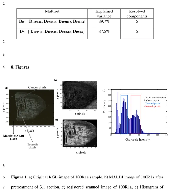
As an example, figure 1a, b and c show an original scanned grayscale image of 100R1a,
19
its related MALDI 2D global intensity map and its corresponding registered scanned
20
image, once binned to the MALDI pixel size, respectively. The scanned image in figure
21
1a reveals three different pixel types according to the gray intensity. Black color pixels
22
correspond to MALDI matrix, the dark gray pixels (external region) are attributed to the
23
region in which tumor cells have grown and light gray pixels (central region)
24
correspond to necrotic tissue.
12
1
FIGURE 1 2
This difference among gray color intensity in the physiological grayscale image was
3
used as a criterion for tissue recognition. Histograms were computed from all the pixels
4
in the physiological grayscale images and the peaks and valleys in the histogram were
5
used to locate the boundaries among clusters related to MALDI matrix, tumor parts and
6
necrotic parts. The tissue assignment in the physiological images was then used to label
7
the related MALDI pixels. Figure 1d shows the histogram corresponding to the
8
registered grayscale image in Figure 1c. The black rectangle includes all the pixels with
9
information of the biological material that was considered for further analysis. The
10
region framed in blue represents the grey intensity range in which tumor parts are
11
clearly located and the red framed region includes the grayscale values associated with
12
necrotic pixels. Pixels with grayscale intensities between both regions were not
13
assigned either to tumor or to necrotic parts to avoid incorrect labeling. Pixels outside
14
the black rectangle are related to background. This background would correspond to
15
MALDI matrix pixels, which give no information; therefore, they were not used for
16
further analysis. It is worth to mention that visually inspection of selected pixels was
17
made to ensure the correct labeling.
18
3.3 Multivariate Curve Resolution—Alternating Least Squares (MCR-ALS) 19
MCR-ALS decomposes the matrix of MS pixel spectra D into a bilinear model, where
20
all MS spectra in the image can be described by the sum of the MS fingerprints of the
21
different pure image constituents weighted according to their relative concentrations in
22
the different pixels. This model is expressed by the following equation in matrix form:
23
D(n,m)=C(n,nc)ST(nc,m)+E(n,m) Equation 1
13
where D (n,m) is the matrix of MS pixel spectra obtained after the pretreatment
1
described in section 3.1, C(n,nc) is the matrix of the relative amounts or concentration
2
of the nc components in the n pixels and ST is the pure MS spectra matrix associated
3
with these nc components. E is the matrix associated with noise or experimental error
4
(variance not explained by the nc resolved components). The indexes n and m refer to
5
the number of pixels analyzed from the image and the number of m/z channels in each
6
MS spectrum, respectively.
7
With the aim to recover the bilinear model expressed in Equation 1, an iterative
8
alternating least squares optimization under constraints is used to obtain both C and ST
9
matrices with a minimum error in the reproduction of the original data set (D). In order
10
to initialize the iterative procedure, a previous determination of the number of pure
11
signal contributions in the raw data set and the generation of C or ST estimates is
12
required.
13
During the alternating least-squares optimization, constraints are used to introduce
14
information useful to provide chemically meaningful C and ST profiles and to decrease
15
the ambiguity in the final solutions obtained [19,27]. In image resolution,
non-16
negativity in the concentration and in the spectral direction are the most commonly used
17
constraints. Normalization of pure spectra in ST is also a common constraint used to
18
avoid scaling fluctuations in the profiles during the optimization. Moreover, the use of
19
local rank constraints can be extremely helpful to improve the reliability of MCR-ALS
20
solutions. Local rank information indicates the absence of one or more constituents in
21
the different pixels. In tissue-based cancer research, local rank information about the
22
presence/absence of different tissues (tumor or necrotic) in samples can be obtained
23
from the grayscale images, as mentioned in section 3.2. In these cases, the use of this
24
physiologically-based local rank information can help to decrease the inherent MCR
14
ambiguity and, consequently, to define better the location and chemical structure of
1
tissue type. The local rank information in terms of compound identification is translated
2
into a ‘mask’ matrix. This matrix, sized as C (n pixels × nc of components), is used
3
to encode the local rank constraints, i.e., the information on the missing components in
4
the different pixels, setting them to have a concentration value equal to zero or smaller
5
than a very low predefined value [19,27].
6
A great advantage of MCR-ALS is the possibility to analyze simultaneously several
7
images in a single multiset structure to provide more reliable results, less affected by
8
ambiguity phenomena [19,28,29]. In a biomedical context, this means that resolved
9
spectral contributions will define much better general trends of the population of
10
samples analyzed together than if images were analyzed individually. In this study, the
11
multiset structure was obtained by appending the pixel MS blocks of the different
12
MALDI images one on top of each other to form a column-wise augmented matrix,
13
Daug. The decomposition Daug = CaugST + E provides a single matrix ST of pure spectra,
14
valid for all the images in the multiset, and a matrix Caug, formed by as many
15
submatrices Ci as images in the multiset. The profiles in each of these Ci submatrices
16
can be refolded conveniently to recover the related distribution maps of every
17
constituent in each image. A multiset structure also obeys the bilinear model seen in
18
Equation 1.
19
The percentage of explained variance is used to indicate the fit quality of the MCR-ALS
20
results. This parameter is calculated according to the expression:
21
∑
∑
ij 2 ij ij * 2 ij 2 d d × 100 = (%) r Equation 2 2215
1
where dij* are the values of the data set reproduced by the bilinear model and dij the
2
original values in the raw data set D. The number of components included in the
MCR-3
ALS model should be compromise between this maximum variance explained by the
4
model, model simplicity, and model interpretability
5
More details about the MCR-ALS method are given in [28,30,31] and a GUI to use the
6
algorithm is freely available at http://mcrals.info.
7 8
3.4 K-means (segmentation analysis) 9
K-means clustering is an algorithm which works by partitioning the observations of a
10
dataset into k clusters [32]. In image analysis, the pixels in the dataset are partitioned
11
into groups according to their similarity, expressed by a similar spectral shape,
12
composition, chemical and/or biological properties.
13
In this study, a single K-means analysis was performed on the 15 images
14
simultaneously. This multiset segmentation analysis allowed finding clusters
15
consistently present in all images and, thus, related to relevant biological structures of
16
the samples analyzed. MCR scores coming from the augmented Caug matrix obtained by
17
MCR-ALS have been used as the pixel input information for K-means analysis because
18
they are excellent compressed and noise-filtered representations of the pixel
19
composition. Besides, each column in Caug has constituent-specific information and this
20
allows performing K-means on some or all the signal contributions resolved by
MCR-21
ALS. When using Caug for segmentation, the number of sought clusters should be equal
22
or slightly higher than the number of MCR contributions used in the K-means analysis.
16
The K-means algorithm basically consists of three steps: 1. Initialization, where few
1
pixels are randomly selected and used as cluster centroids. 2. Assignment of every pixel
2
of the data set to its nearest centroid, and 3. Updating of the centroid position based on
3
the groups formed. Steps 2 and 3 are iteratively performed until centroids do not shift
4
any longer and clusters are stable or when a present number of iterations is exceeded. In
5
this work, 100 replicates with random initial centroid positions were performed to
6
achieve more reliable results and Euclidean distance was used as a similarity criterion
7
for pixel assignment to clusters. Finally, suitable segmentation maps were obtained
8
refolding the part of the segmentation vector that relates to each image. Segmentation
9
maps can be used to be compared with physiological images.
10
Moreover, the use of MCR scores provides chemically meaningful spectra of the
11
components and, hence, allows interpreting easily the centroid properties in each
12
segmentation class. This is an advantage in comparison with the centroids coming from
13
PCA scores, which are difficult to interpret because these composition-related values
14
are abstract and lack chemical sense.
15
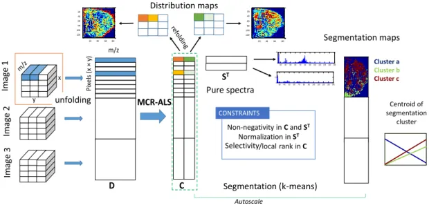
Figure 2 presents a schematic illustration of the combination of MCR-ALS with
K-16
means for the simultaneous analysis of MALDI images previously described. First,
17
multiset MCR-ALS is applied to the images of biological tissues to provide basic
18
spectral signatures and distribution maps of the biological contributions. Finally,
19
multiset K-means analysis is applied to obtain consistent tissue clusters (relevant
20
biological parts) common to all samples. MCR scores from biological constituents in
21
MSI images were used as input pixel information for segmentation analysis.
22
Autoscaling was applied to each concentration profile in each submatrix Ci of the Caug
23
matrix, to balance the importance of all biological constituents present in each image in
17
the segmentation analysis. This strategy might be considered as generally applicable for
1
mass spectrometry imaging data analysis.
2 3
FIGURE 2 4
4. Results and discussion 5
This section will include the results obtained from both image resolution and
6
segmentation approaches. Firstly, the information gathered from the comparison of the
7
analysis of the two types of tumor by MCR-ALS will be showed. Secondly, advantages
8
of the implementation of the new constraint in the simultaneous MCR-ALS analysis of
9
all 15 images will be presented. Finally, the results achieved from the multiset image
10
segmentation and a final interpretation of the chemical results will be offered. 4.1.
11
Resolution analysis (MCR-ALS) 12
The first MCR-ALS analysis was oriented to identify significant contributions with a
13
specific “mass signature” for each tumor type (R or S). To do so, two multisets as
14
described in section 3.3. were built, each containing images related to a particular kind
15
of tumor and were analyzed separately. The first multiset was formed by the four
16
images corresponding to the tumors of 100% R, DaugR= [D100R1a; D100R1b; D100R1c;
17
D100R2], and the second multiset by the four images corresponding to the tumors of
18
100% S, DS= [ D100S3a; D100S3b; D100S3c; D100S4].
19
MCR-ALS was applied separately to each multiset structure (DR and DS) following the
20
steps explained in section 3.3 and the following bilinear models were obtained:
21
DaugR = CaugR*STR Equation 2
22
DaugS = CaugS*STS Equation 3
18
and using non-negativity constraints in concentration and spectra profiles and spectra
1
normalization in matrix STR or S (using the Euclidean norm).
2
Table 2 lists the number of resolved components and the explained variance obtained
3
from the MCR-ALS analyses of both multisets. Resolution of five contributions was
4
necessary in both cases. The inclusion of a different number of contributions gave
5
worse data fits or unreliable spectra or distribution maps (see Figure S1 in
6
Supplementary information for resolved spectra and distribution maps for these two
7
MCR-ALS analyses). Four contributions were related to biological regions of the
8
tissues; two associated with tumoral parts and two corresponding to necrotic parts,
9
according to the morphology seen in the related grayscale images. The need of two
10
biological contributions to describe the tumoral part of the sample and two additional
11
ones for the description of the necrotic regions of the samples is not surprising if we
12
take into consideration the heterogeneity associated with this kind of tissues. Moreover,
13
an additional non-biological contribution was needed to improve the resolution results
14
in both multiset structures. This extra contribution could be attributed to instrumental
15
background or could be originated to compensate for variations linked to slight
16
differences of sample preparation. Actually, the high noise of MSmass spectra and
17
possible experimental differences in the tissue preparation also justify that the explained
18
variance by the models does not exceed 90%.
19 20
TABLE 2 21
22
A correlation coefficient matrix generated by comparing by pairs the resolved spectra of
23
the components of both multisets (STR and STS) by Pearson correlation shows a high
19
correlation between analogous biological components of the two tumor cell lines R and
1
S (see correlation matrix shown below).
2 3
4
Where Rc1/Rc2 and Sc1/Sc2 were the spectra corresponding to tumoral contribution 1/2
5
of DR and DS, respectively. Rn1/Rn2 and Sn1/Sn2 were the spectra corresponding to
6
necrotic contribution 1/2 of DR and DS, respectively. Finally, Rb and Sb were the
7
spectra corresponding to background contribution of DR and DS, respectively.
8
No significant differences between the composition of tumors R and S were found.
9
Thus, resolved mass spectral signatures of the four biological contributions related to
10
tumor and necrotic parts were rather similar in both R and S tumoral tissues. Indeed, in
11
tumoral contributions, Rc and Sc, correlation coefficient values were equal or higher
12
than 0.9, whereas the lowest correlation coefficient between necrotic contributions, Rn
13
and Sn, was 0.8. Only the non-biological contributions, Rb and Sb, presented expected
14
differences in the spectral signatures, due to the noise random nature. Limits in the
15
selectivity of the MS detection system and the fact that both R and S clones are closely
16
related, since they derived from the same original HCT116 cell line, could be the
17
reasons to explain why a specific distinction and identification of “mass signatures” for
18
each tumor type was not possible. Owing to this limitation, the interpretation of the
19
differences among the R and S tumor compounds obtained was no longer the main goal
20 Rc1 Rc2 Rn1 Rn2 Rb Sc1 0,9 0,0 0,4 0,1 0,0 Sc2 0,0 1,0 0,1 0,1 -0,1 Sn1 0,6 0,0 0,8 0,4 0,4 Sn2 0,1 0,2 0,7 0,9 -0,1 Sb 0,5 0,0 0,6 0,4 0,2
20
of the work. However, some general interpretation, valid for R and S tumors, can still be
1
done. Therefore, salient masses in the tumor signatures to masses around 750-800 could
2
be assigned to glycosyldiradylglycerols, glycerophosphocholines or
3
glycerophosphoglycerols and around 520-525 with oxidized glycerophospholipids or
4
fatty acyl glycosides. Relevant masses in the necrotic signatures to masses around
400-5
430 could be assigned to sterols/fatty esters.
6
The spectral similarity between both tumors R and S suggested the possibility of
7
performing a simultaneous treatment of all 15 images corresponding to homogeneous
8
(100% R or S) and heterogenous (different percentages of R and S) tumor tissues in
9
order to obtain more reliable mass spectral signatures and distribution maps to integrally
10
describe the tumor and necrotic contributions common to both kind of R and S tumor
11
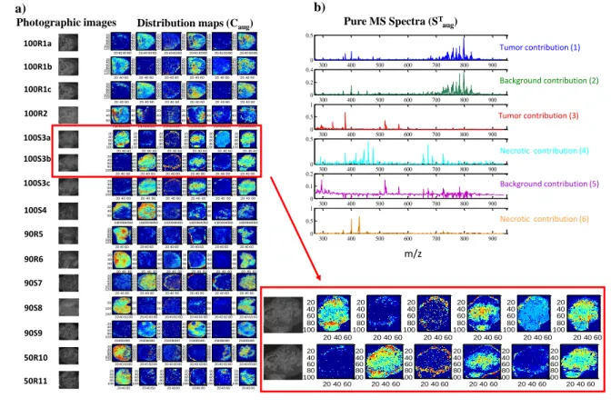
samples [19,28,29]. Therefore, MCR-ALS analysis of the multiset formed by the 15
12
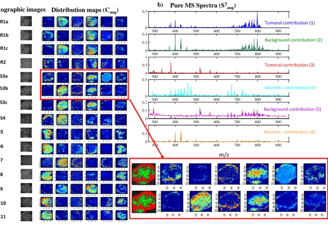
images was performed. Figures 3a and b show the MCR-ALS resolved distribution
13
maps and pure spectra of the analyzed multiset. Results were clearly showed through
14
the example of two images (100S3a and 100S3b) with a higher magnification and the
15
full set of magnified distribution maps were provided as supplementary information (see
16
Figure S2). Related scanned grayscale images of all samples analyzed with MSI are also
17
shown (left plots in figure 3a). As mentioned in section 3.2, these physiological
18
grayscale pictures show the region in which tumoral cell populations have grown (dark
19
gray color) and the region where necrosis has been produced (light gray color).
20
Therefore, these grayscale images help to associate each resolved MCR contribution
21
with a particular kind of tissue types (tumoral or necrotic). A
22 23
FIGURE 3 24
21
1
Now, in contrast to the analysis of either DR or DS multiset structures, resolution of six
2
components is proposed. As in the resolution of DR and DS multisets, the four
3
components associated with relevant biological parts (tumor and necrotic) were
4
observed. Looking at their related grayscale images, blue (component 1) and red
5
(component 3) could be approximately associated with tumor contributions and cyan
6
(component 4) and orange (component 6) with necrotic contributions. Moreover, two
7
non-biological contributions (green and violet) were again required to perform the
8
analysis and to cope with spectral differences due to instrumental and experimental
9
variability. As expected, two non-biological spectral contributions were needed instead
10
of one, in agreement with the lack of correlation between the Rb and Sb contribution
11
resolved in the DR and DS multisets.
12
After the preliminary simultaneous MCR-ALS analysis of all 15 images, visual
13
inspection of the distribution maps showed that the contributions 1 (blue) and 6 (orange)
14
corresponding to a tumor contribution and a necrotic contribution, respectively, were
15
blending with each other throughout the resolution. In some images corresponding to
16
homogenous tumors (both 100% R and 100% S) the tumor contribution 1 was found in
17
regions associated with necrotic tissue that should not be present and likewise for the
18
necrotic contribution 6 that was present in parts of the tissues attributed to tumor tissue
19
(see distribution maps of Figure 3).
20
The preliminary MCR-ALS analysis of the fifteen images was not fully satisfactory but
21
provided better spectral signatures for the contributions to be modelled than the raw
22
image and an approximate identification of the biological and non-biological
23
contributions of the data set. The resolved spectral signatures were used as initial
24
estimates in a second MCR-ALS analysis and the information provided by the
22
concentration profiles was used as an auxiliary source of information to set local rank
1
constraints, as described below.
2
Since spatial information of tumor and necrotic parts can be identified in the grayscale
3
images of tissue slices, this information was used to force the presence/absence of
4
tumor/necrotic contributions throughout the resolution. Once tumor and necrotic pixels
5
were identified using the image registration between grayscale and MS images (See
6
section 3), a masking local rank matrix was built to be used as a constraint (see section
7
3.2 for more detail in the implementation of this constraint). Taking as a basis the
8
preliminary results obtained by MCR-ALS analysis using only non-negativity
9
constraints, pixels related to necrotic parts were forced to be absent in component 1
10
(blue tumor contribution) and pixels corresponding to tumor cell populations were
11
forced to be absent in component 6 (orange necrotic contribution) in the images
12
corresponding to both 100% R and 100 % S. Please note that the use of this constraint
13
does not need either that all pixels in all images be constrained nor that all biological
14
contributions be subject to local rank conditions. The use of this constraint in small
15
areas clearly characterized as necrotic or tumor in simpler samples, such as 100% R or
16
100% S, is sufficient to improve significantly the results of the whole multiset.
17
Figure 4 shows the resolution results for the simultaneous analysis of all 15 images
18
using non-negativity, normalization and local rank information. The variance explained
19
obtained in the resolution using only non-negativity and normalization constraints was
20
86.8 % and now with the use of the local rank constraint is 85.5 %. The similarity
21
between the two values indicates that the new constraint introduced is correct and does
22
not perturb the natural behavior of the data set. Resolved distribution maps
23
corresponding to 100S3a and 100S3b were again zoomed for better visualization and
24
the full set of magnified distribution maps were provided as supplementary information
23
(see Figure S3). Moreover, pixel selection from the registered scanned images of
1
necrotic (green color) and tumoral regions (red color) were also showed for these two
2
examples (left side of the zoomed plot in Figure 4).
3 4
FIGURE 4 5
6
By examination of the MCR-ALS results, the positive effect of local rank constraints in
7
the definition of MS signatures and in the morphology of the distribution maps of the
8
different biological contributions can be clearly seen . Now, in contrast to the resolution
9
only using non-negativity and normalization constraints, tumor contribution 1 and
10
necrotic contribution 6 are no longer mixed with each other and are located in their
11
correct physiological regions. Besides, the resolved profiles are more accurate and show
12
less ambiguity due to the effect of the local rank constraint.
13
Once the MCR-ALS analysis on the all 15 images was performed, the MCR scores
14
(Caug, distribution maps of sample constituents) were used for segmentation analysis.
15 16
4.2 Multiset image segmentation. K-means cluster analysis. 17
Multiset image segmentation analysis was the next step in the strategy proposed (see
18
figure 2), mainly performed to look for clusters present in all analyzed images. As
19
mentioned before, K-means analysis was carried out using resolved MCR scores of the
20
multiset structure (see Figure 4). The fact of using MCR scores allows selecting the
21
information to be included in the segmentation process. In this case, only the four
22
biological contributions related to tumor and necrotic parts (contributions 1, 3, 4 and 6)
23
were selected and the background contributions (2 and 5) were left aside.
24
The individual profiles of the four biological contributions of each submatrix Ci of the
1
Caug matrix were autoscaled to balance the importance of each biological contribution
2
present in each image of the multiset in the segmentation analysis. Doing it by block
3
(each Ci separately), global intensity differences among MS images were also
4
compensated. Autoscaled concentration profiles Ci were segmented simultaneously into
5
four classes. In this case, a number of clusters equal to the number of biological
6
contributions was selected. No reliable patterns of necrotic and cancer regions were
7
achieved when the number of clusters in the segmentation procedure was increased.
8
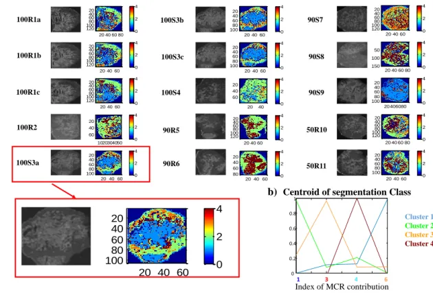
Figure 5 shows the segmentation results obtained by using the preprocessed MCR
9
scores previously described. Zoom in an example (image 100S3a) was provided in
10
Figure 5 for a better evaluation of the results and magnified results of the full set can be
11
seen in supplementary information (see Figure S4).
12 13
FIGURE 5 14
15
The fact that K-means assign each pixel to only one cluster [32] helps to attribute that
16
cluster to a single tissue type and, hence, be more easily comparable with the grayscale
17
images. In figure 5 grayscale images were presented (left side of the pair images in
18
Figure 5) for comparison with their related segmentation maps (right side of the pair
19
images in Figure 5). It can be observed that the grayscale images match the location of
20
tumor and necrotic parts with their related segmentation maps. Clusters 2 (green) and 3
21
(orange) correspond to the tumor parts, they have the same spatial distribution of the
22
dark grey regions in the scanned image. Similarly, cluster 1 (blue) and 4 (brown) were
23
associated with the necrotic parts. However, this information is richer than that provide
25
by the grayscale images, since heterogeneity within the same kind of tissue (tumor or
1
necrotic) can be appreciated.
2
Centroid profiles using MCR scores in segmentation analysis are interpretable and,
3
hence, it is possible to know which component or mixture of components is represented
4
in each cluster. In our case, cluster 2 and 3 display dominance of contribution 1 and 3 of
5
MCR contributions (tumor contributions), respectively, and low relative presence of
6
other compounds, as expected. Likewise, cluster 1 and 4 show dominance of
7
contribution 4 and 6 of MCR contributions (necrotic contributions). It must be reminded
8
that segmentation clusters can be potentially formed by pure compound pixels or by
9
pixel mixtures, whereas distribution maps from image resolution display the distribution
10
of each pure image constituent. Since image constituents overlap (specially species 1
11
and 4), clusters are formed by some pixels with constituent mixtures of different
12
composition. As mentioned before, an important asset is that MCR scores only include
13
information related to biological contributions of the samples and discard information
14
associated with background contributions. This benefit cannot be obtained if
15
segmentation procedures are directly applied to raw MS image spectra.
16
The results from the combination of MCR with segmentation analysis could be
17
potentially compared with conventionally stained sections to support determination of
18
both anatomical and histopathological features and to provide a better chemical
19
characterization of the compounds or mixtures of compounds involved in every sample
20
region.
21
In future works, the incorporation of more selective MS detection systems and the use
22
of conventionally stained sections is planned to allow for a more specific identification
23
and location of biological regions to incorporate local rank constraints and for a better
24
definition of the MS spectral signatures obtained to describe tumor heterogeneity.
26
1
5. Conclusions 2
The strategy of combining multiset resolution and segmentation has been shown to
3
work for the analysis of biological tissues based on the use of hyperspectral images. For
4
the first time, this strategy was applied to MALDI-MSI data and spatial information
5
from grayscale images was used to set local rank constraints in the MCR-ALS
6
resolution. This constraint improved significantly the morphology of the constituent
7
distributions maps resolved by the MCR-ALS, helped in the suppression of the
8
ambiguity in the results obtained and, therefore, contributed to a better definition of the
9
related MS signatures for every biological contribution.
10
From the grayscale images, relevant features corresponding to anatomical areas of
11
interest (tumoral or necrotic areas) could be identified. The use of this information to
12
force certain components to be absent in particular pixels through MCR-ALS multiset
13
analysis allowed providing reliably spectral signatures to define biological parts
14
common in all the samples and to provide MCR scores for subsequent segmentation
15
analysis. The results of image segmentation distinguished different tissue types (within
16
tumor or necrotic areas) and their spatial distribution matched consistently with the
17
grayscale images. Therefore, the segmentation maps and the chemical information
18
linked to them could be eventually compared with the outcomes of standard
19
histopathological staining protocols.
20
It is essential to stress the twofold benefit of using in a combined way physiological
21
grayscale images and MSI measurements. On the one hand, the results obtained from
22
MSI analysis by MCR-ALS are clearly improved by the easy setting of local rank
23
constraints based on the visual location of different tissues in grayscale images. On the
27
other hand, the plain information in grayscale images, only marking the boundaries
1
among tissue regions, is greatly enhanced by the MS signatures provided after
MCR-2
ALS application associated with the different tissue regions. Such a detailed MSI
3
analysis also provides more insight on the intrinsic heterogeneity of tissue regions, often
4
necessarily described by more than one biological contribution.
5
The strategy proposed was shown to work for a case study including fifteen
6
experimental tumors with different grade of heterogeneity but can be generally
7
applicable in any study of biological material based on mass spectrometry imaging data
8 analysis. 9 10 6. Acknowledgements 11
This work is part of the BEST Postdoctoral Program, funded by the European
12
Commission under Horizon 2020’s Marie Skłodowska-Curie Actions COFUND
13
scheme (Grant Agreement no. 712754) and by the Severo Ochoa program of the
14
Spanish Ministry of Science and Competitiveness (Grant SEV-2014-0425 (2015-2019)).
15
A.J. acknowledges financial support from the Catalan government through project 2017
16
SGR 753 and the Spanish government through project CTQ2015-66254-C2-2-P.7. We
17
would like to acknowledge, the Departament d’Universitats, Recerca i Societat de la
18
Informació de la Generalitat de Catalunya (expedient 2017 SGR 1721); the Comissionat
19
per a Universitats i Recerca del DIUE de la Generalitat de Catalunya; and the European
20
Social Fund (ESF). Additional financial support has been provided by the Institut de
21
Bioenginyeria de Catalunya (IBEC). IBEC is a member of the CERCA
22
Programme/Generalitat de Catalunya. This publication has been also funded with
28
support from the French National Research Agency under the program “Investissements
1
d’avenir” Grant Agreement LabEx MAbImprove: ANR-10-LABX-53.
2 3
References 4
[1] E.H. Seeley, R.M. Caprioli, MALDI imaging mass spectrometry of human tissue:
5
Method challenges and clinical perspectives, Trends Biotechnol. 29 (2011) 136–
6
143. doi:10.1016/j.tibtech.2010.12.002.
7
[2] R.R. Drake, T.W. Powers, E.E. Jones, E. Bruner, A.S. Mehta, P.M. Angel,
8
MALDI Mass Spectrometry Imaging of N-Linked Glycans in Cancer Tissues, 1st
9
ed., Elsevier Inc., 2017. doi:10.1016/bs.acr.2016.11.009.
10
[3] T.J.A. Dekker, B.D. Balluff, E.A. Jones, C.D. Schöne, M. Schmitt, M. Aubele,
11
J.R. Kroep, V.T.H.B.M. Smit, R.A.E.M. Tollenaar, W.E. Mesker, A. Walch, L.A.
12
McDonnell, Multicentre matrix-assisted laser desorption/ionization mass
13
spectrometry imaging (MALDI MSI) identifies proteomic differences in breast
14
cancer-associated stroma., J. Proteome Res. (2014). doi:10.1021/pr500253j.
15
[4] A. Buck, S. Halbritter, C. Späth, A. Feuchtinger, M. Aichler, H. Zitzelsberger,
16
K.P. Janssen, A. Walch, Distribution and quantification of irinotecan and its
17
active metabolite SN-38 in colon cancer murine model systems using MALDI
18
MSI, Anal. Bioanal. Chem. 407 (2015) 2107–2116.
doi:10.1007/s00216-014-19
8237-2.
20
[5] * Richard M. Caprioli, and Terry B. Farmer, J. Gile, Molecular Imaging of
21
Biological Samples: Localization of Peptides and Proteins Using MALDI-TOF
22
MS, 69 (1997) 4751–4760. doi:10.1021/AC970888I.
29
[6] T. Alexandrov, MALDI imaging mass spectrometry: statistical data analysis and
1
current computational challenges., BMC Bioinformatics. 13 Suppl 1 (2012) S11.
2
doi:10.1186/1471-2105-13-S16-S11.
3
[7] H.B. Mann, D.R. Whitney, On a Test of Whether one of Two Random Variables
4
is Stochastically Larger than the Other, Ann. Math. Stat. 18 (1947) 50–60.
5
doi:10.1214/aoms/1177730491.
6
[8] M. Hanselmann, M. Kirchner, B.Y. Renard, E.R. Amstalden, K. Glunde, R.M.A.
7
Heeren, F.A. Hamprecht, Concise representation of mass spectrometry images by
8
probabilistic latent semantic analysis, Anal. Chem. 80 (2008) 9649–9658.
9
doi:10.1021/ac801303x.
10
[9] H.C. Diehl, B. Beine, J. Elm, D. Trede, M. Ahrens, M. Eisenacher, K. Marcus,
11
H.E. Meyer, C. Henkel, The challenge of on-tissue digestion for MALDI MSI- a
12
comparison of different protocols to improve imaging experiments, Anal.
13
Bioanal. Chem. 407 (2015) 2223–2243. doi:10.1007/s00216-014-8345-z.
14
[10] Y. Gut, M. Boiret, L. Bultel, T. Renaud, A. Chetouani, A. Hafiane, Y.M. Ginot,
15
R. Jennane, Application of chemometric algorithms to MALDI mass
16
spectrometry imaging of pharmaceutical tablets, J. Pharm. Biomed. Anal. 105
17
(2015). doi:10.1016/j.jpba.2014.11.047.
18
[11] C. Bedia, R. Tauler, J. Jaumot, Analysis of multiple mass spectrometry images
19
from different Phaseolus vulgaris samples by multivariate curve resolution,
20
Talanta. 175 (2017) 557–565. doi:10.1016/j.talanta.2017.07.087.
21
[12] J. Jaumot, R. Tauler, Potential use of multivariate curve resolution for the
22
analysis of mass spectrometry images, Analyst. 140 (2015).
23
doi:10.1039/c4an00801d.
30
[13] D. Trede, S. Schi, M. Becker, S. Wirtz, K. Steinhorst, J. Strehlow, M. Aichler,
1
J.H. Kobarg, J. Oetjen, A. Dyatlov, S. Heldmann, A. Walch, H. Thiele, P. Maass,
2
T. Alexandrov, Excluído-Exploring Three-Dimensional Matrix-Assisted Laser
3
Desorption/ Ionization Imaging Mass Spectrometry Data: Three-Dimensional
4
Spatial Segmentation of Mouse Kidney, Anal. Chem. 84 (2012) 6079–6087.
5
[14] T. Alexandrov, J.H. Kobarg, Efficient spatial segmentation of large imaging mass
6
spectrometry datasets with spatially aware clustering, Bioinformatics. 27 (2011)
7
i230–i238. doi:10.1093/bioinformatics/btr246.
8
[15] S. Piqueras, L. Duponchel, R. Tauler, A. De Juan, Resolution and segmentation
9
of hyperspectral biomedical images by Multivariate Curve
Resolution-10
Alternating Least Squares, Anal. Chim. Acta. 705 (2011) 182–192.
11
doi:10.1016/j.aca.2011.05.020.
12
[16] S. Piqueras, C. Krafft, C. Beleites, K. Egodage, F. von Eggeling, O.
Guntinas-13
Lichius, J. Popp, R. Tauler, A. de Juan, Combining multiset resolution and
14
segmentation for hyperspectral image analysis of biological tissues, Anal. Chim.
15
Acta. 881 (2015) 24–36. doi:10.1016/j.aca.2015.04.053.
16
[17] J. Felten, H. Hall, J. Jaumot, R. Tauler, A. de Juan, A. Gorzsás, Vibrational
17
spectroscopic image analysis of biological material using multivariate curve
18
resolution–alternating least squares (MCR-ALS), Nat. Protoc. 10 (2015) 217–
19
240. doi:10.1038/nprot.2015.008.
20
[18] J. Jaumot, R. Tauler, MCR-BANDS: A user friendly MATLAB program for the
21
evaluation of rotation ambiguities in Multivariate Curve Resolution, Chemom.
22
Intell. Lab. Syst. 103 (2010) 96–107. doi:10.1016/j.chemolab.2010.05.020.
23
[19] R. Tauler, A. Smilde, B. Kowalski, Selectivity, local rank, three‐way data
31
analysis and ambiguity in multivariate curve resolution, J. Chemom. 9 (1995)
1
31–58. doi:10.1002/cem.1180090105.
2
[20] A. De Juan, M. Maeder, T. Hancewicz, R. Tauler, Use of local rank-based spatial
3
information for resolution of spectroscopic images, J. Chemom. 22 (2008) 291–
4
298. doi:10.1002/cem.1099.
5
[21] X. Zhang, A. De Juan, R. Tauler, Local rank-based spatial information for
6
improvement of remote sensing hyperspectral imaging resolution, Talanta. 146
7
(2016) 1–9. doi:10.1016/j.talanta.2015.08.017.
8
[22] L. Candeil, I. Gourdier, D. Peyron, N. Vezzio, V. Copois, F. Bibeau, B. Orsetti,
9
G.L. Scheffer, M. Ychou, Q.A. Khan, Y. Pommier, B. Pau, P. Martineau, M. Del
10
Rio, ABCG2 overexpression in colon cancer cells resistant to SN38 and in
11
irinotecan-treated metastases, Int. J. Cancer. 109 (2004) 848–854.
12
doi:10.1002/ijc.20032.
13
[23] C. Gongora, N. Vezzio-Vie, S. Tuduri, V. Denis, A. Causse, C. Auzanneau, G.
14
Collod-Beroud, A. Coquelle, P. Pasero, P. Pourquier, P. Martineau, M. Del Rio,
15
New Topoisomerase I mutations are associated with resistance to camptothecin,
16
Mol. Cancer. 10 (2011) 1–13. doi:10.1186/1476-4598-10-64.
17
[24] S. Gibb, K. Strimmer, Maldiquant: A versatile R package for the analysis of mass
18
spectrometry data, Bioinformatics. 28 (2012) 2270–2271.
19
doi:10.1093/bioinformatics/bts447.
20
[25] M.H.Ã. Zhu, L.G. Liu, Y.S. Cheng, T.K. Dong, Z. You, A.A. Xu, Nuclear
21
Instruments and Methods in Physics Research A Iterative estimation of the
22
background in noisy spectroscopic data, 602 (2009) 597–599.
23
doi:10.1016/j.nima.2009.01.174.
32
[26] B.G. Sharma, A. Thé, Automating Image Registration with MATLAB,
1
Mathworks.Com. (2013) 1–7.
2
[27] a. de Juan, R. Tauler, Chemometrics applied to unravel multicomponent
3
processes and mixtures, Anal. Chim. Acta. 500 (2003) 195–210.
4
doi:10.1016/S0003-2670(03)00724-4.
5
[28] R. Tauler, Multivariate curve resolution applied to second order data, Chemom.
6
Intell. Lab. Syst. 30 (1995) 133–146. doi:10.1016/0169-7439(95)00047-X.
7
[29] R. Tauler, M. Maeder, A. de Juan, Multiset Data Analysis: Extended Multivariate
8
Curve Resolution, in: Compr. Chemom., Elsevier, 2009: pp. 473–505.
9
doi:10.1016/B978-044452701-1.00055-7.
10
[30] R. de Juan, Anna; Rutan, S. and Tauler, Two-Way Data Analysis: Multivariate
11
Curve Resolution – Iterative Resolution Methods, in: B. Brown, S. D. ; Tauler, R.
12
and Walczak (Ed.), Compr. Chemom., Elsevier, 2010: pp. 325–344.
13
[31] J. Jaumot, A. de Juan, R. Tauler, MCR-ALS GUI 2.0: New features and
14
applications, Chemom. Intell. Lab. Syst. 140 (2015).
15
doi:10.1016/j.chemolab.2014.10.003.
16
[32] T.N. Tran, R. Wehrens, L.M.C. Buydens, Clustering multispectral images: a
17
tutorial, Chemom. Intell. Lab. Syst. 77 (2005) 3–17.
18 doi:10.1016/j.chemolab.2004.07.011. 19 20 21 22
33 1 2 3 4 5
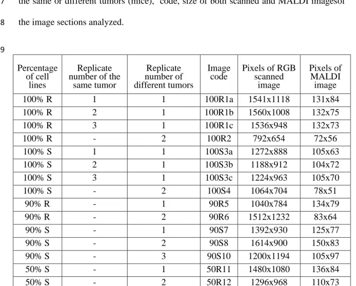
Table 1. Percentage of both R and S cell lines in xenografts, replicate number of either 6
the same or different tumors (mice), code, size of both scanned and MALDI imagesof
7
the image sections analyzed.
8 9 Percentage of cell lines Replicate number of the same tumor Replicate number of different tumors Image
code Pixels of RGB scanned image Pixels of MALDI image 100% R 1 1 100R1a 1541x1118 131x84 100% R 2 1 100R1b 1560x1008 132x75 100% R 3 1 100R1c 1536x948 132x73 100% R - 2 100R2 792x654 72x56 100% S 1 1 100S3a 1272x888 105x63 100% S 2 1 100S3b 1188x912 104x72 100% S 3 1 100S3c 1224x963 105x70 100% S - 2 100S4 1064x704 78x51 90% R (10% S) - 1 90R5 1040x784 134x79 90% R (10% S) - 2 90R6 1512x1232 83x64 90% S (10% R) - 1 90S7 1392x930 125x77 90% S (10% R) - 2 90S8 1614x900 150x83 90% S (10% R) - 3 90S10 1200x1194 105x97 50% S (50% R) - 1 50R11 1480x1080 136x84 50% S (50% R) - 2 50R12 1296x968 110x73 10 11
Table 2. Number of resolved components and variance explained by MCR-ALS 12
analysis of Dr and Ds multiset structures.