HAL Id: insu-02271293
https://hal-insu.archives-ouvertes.fr/insu-02271293
Submitted on 9 Sep 2019
HAL is a multi-disciplinary open access
archive for the deposit and dissemination of
sci-entific research documents, whether they are
pub-lished or not. The documents may come from
teaching and research institutions in France or
abroad, or from public or private research centers.
L’archive ouverte pluridisciplinaire HAL, est
destinée au dépôt et à la diffusion de documents
scientifiques de niveau recherche, publiés ou non,
émanant des établissements d’enseignement et de
recherche français ou étrangers, des laboratoires
publics ou privés.
Building a Weakly Outgassing Comet from a
Generalized Ohm’s Law
J. Deca, Pierre Henri, A Divin, A. Eriksson, M. Galand, A. Beth, K.
Ostaszewski, M. Horányi
To cite this version:
J. Deca, Pierre Henri, A Divin, A. Eriksson, M. Galand, et al.. Building a Weakly Outgassing Comet
from a Generalized Ohm’s Law. Physical Review Letters, American Physical Society, 2019, 123 (5),
�10.1103/PhysRevLett.123.055101�. �insu-02271293�
Jan Deca∗
Laboratory for Atmospheric and Space Physics (LASP), University of Colorado Boulder, Boulder, Colorado 80303, USA and
Institute for Modeling Plasma, Atmospheres and Cosmic Dust, NASA/SSERVI, Moffet Field, California 94035, USA
Pierre Henri
LPC2E, CNRS, Orl´eans, 45071, France
Andrey Divin
Physics Department, St. Petersburg State University, St. Petersburg, 198504, Russia
Anders Eriksson
Swedish Institute of Space Physics (IRF), Uppsala 751 21, Sweden
Marina Galand and Arnaud Beth
Department of Physics, Imperial College London, London SW7 2AZ, UK
Katharina Ostaszewski
Institute for Geophysics and Extraterrestrial Physics (IGeP), Technische Universtit¨at Braunschweig, Braunschweig 38106, Germany
Mih´aly Hor´anyi
Laboratory for Atmospheric and Space Physics (LASP), University of Colorado Boulder, Boulder, Colorado 80303, USA
Institute for Modeling Plasma, Atmospheres and Cosmic Dust, NASA/SSERVI, Moffet Field, California 94035, USA and
Department of Physics, University of Colorado Boulder, Boulder, Colorado 80309, USA (Dated: August 20, 2019)
When a weakly outgassing comet is sufficiently close to the Sun, the formation of an ionized coma results in solar wind mass loading and magnetic field draping around its nucleus. Using a 3D fully kinetic approach, we distill the components of a generalized Ohm’s law and the effective electron equation of state directly from the self-consistently simulated electron dynamics and identify the driving physics in the various regions of the cometary plasma environment. Using the example of space plasmas, in particular multi-species cometary plasmas, we show how the description for the complex kinetic electron dynamics can be simplified through a simple effective closure, and identify where an isotropic single-electron fluid Ohm’s law approximation can be used, and where it fails.
Numerical models that seek to describe the evolution 1
of plasma without self-consistently including the electron 2
dynamics, such as (multi-)fluid and hybrid simulation 3
approaches [1], need to rely on a relation that prescribes 4
the behavior of the unresolved species. Typically a 5
generalized Ohm’s law (GOL) is assumed [2], combined 6
with a closure relation such as a polytropic or a double 7
adiabatic evolution [3, 4]. In this letter, we show how a 8
GOL can unravel the hidden mysteries of multi-species 9
plasma environments, such as the solar wind plasma 10
interaction with a weakly outgassing comet [5–7]. We 11
indicate where reduced plasma models can be applied, 12
e.g., to gain more direct access to the ongoing physics 13
and/or to decrease the needed amount of computational 14
resources, and show the consequences of this compromise. 15
∗mailto: [email protected]
16
The Rosetta spacecraft caught up with comet 17
67P/Churyumov-Gerasimenko (hereafter 67P) at a 18
heliocentric distance of 3.6 AU [8, 9]. At a few hundreds 19
of kilometers from the cometary nucleus, the Rosetta 20
plasma instruments, quite unexpectedly, picked up 21
the signatures of a plasma environment dominated 22
by cometary matter [10, 11], even though 67P had an 23
outgassing rate of one to two orders of magnitude smaller 24
than 1P/Halley at a similar heliocentric distance [12–15]. 25
This meant that even at large heliocentric distances the 26
weakly outgassing nucleus of 67P mass-loads the solar 27
wind plasma [5, 6]. 28
29
Various ionization processes, such as electron-impact 30
ionization, photo-ionization, and charge exchange, 31
contribute to the shape of the near-cometary environ-32
ment [16–18]. Rosetta observed a radial dependence of 33
2
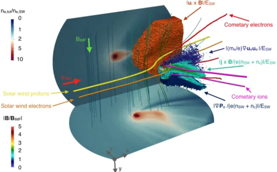
FIG. 1. Illustration of the solar wind interaction with a weakly outgassing comet rep-resentative of 67P/Churyumov-Gerasimenko at a heliocentric distance of 4.0 − 4.5 AU. For each simulated species, velocity streamlines representative of its dynamics are plotted. The var-ious isovolumes represent where the respective components of the generalised Ohm’s law are significant with respect to the four-fluid behavior of the sys-tem. The projections repre-sent the total electron density on two perpendicular planes through the center of the nu-cleus. Refer to Fig. 2 for exact numbers and scaling.
the plasma density with distance from the nucleus [19, 20] 34
or, in other words, there exists a continuously changing 35
ratio between the cometary and the upstream solar wind 36
plasma density throughout 67P’s plasma environment, 37
both along the Sun-comet direction as well as in the 38
meridian plane [21–23]. To first order, for a weakly 39
outgassing comet, the dynamical interaction that de-40
termines the general structure of the cometary plasma 41
environment is representative of a four-fluid coupled 42
system (illustrated in Fig. 1), where the solar wind 43
electrons move to neutralize the cometary ions and the 44
cometary electrons organize themselves to neutralize the 45
solar wind ions [7]. 46
47
In addition to a detailed understanding of the kinetic 48
dynamics that governs the solar wind interaction with 49
a weakly outgassing comet, in this letter we provide 50
feedback to (multi-)fluid [24–29] and hybrid [16, 30–37] 51
models where the electrons dynamics is prescribed 52
through a GOL combined with an electron closure 53
relation. Using a fully kinetic, self-consistent approach 54
for the electron dynamics, however, we can work the 55
other way around and compute the various terms of 56
the GOL directly from the simulation output. Our 57
simulation model does not assume any GOL. This allows 58
us to identify the compromises that a simplified electron 59
pressure tensor brings to the electron dynamics and 60
to establish where it is justified to adopt a GOL that 61
mimics the electron dynamics. As the locations of the 62
solar wind and cometary species in phase space changes 63
throughout the cometary plasma environment, so will 64
the balance between the different contributions to the 65
total electric field in the GOL in response to the physical 66
processes that dominate each region. 67
68
To simulate the solar wind interaction with comet 67P 69
Plasma parameters Te,sw[eV] 10 ne,sw[cm−3] 1
Tp,sw[eV] 7 np,sw[cm−3] 1
Te,c[eV] 10 vsw[km s−1] 400
Tp,c[eV] 0.026 ωpl,e[rad s−1] 13165
mp,sw/me,sw 100 BIMF[nT] 6 mp,c/mp,sw 20 Q [s−1] 1025 Simulation setup Domain size [km3] 3200×2200×2200 Resolution [km3] 10×10×10 Time step [s] 4.5×10⁻⁵
TABLE I. Overview of the plasma parameters and setup of the computational domain. The subscripts ‘e, sw’ and ‘e, c’ represent solar wind and cometary electron quantities, respec-tively, and ‘p, sw’ and ‘p, c’ represent solar wind proton and cometary ion quantities, respectively. ωpl,e is the upstream
electron plasma frequency.
we use the semi-implicit, fully kinetic, electromagnetic 70
particle-in-cell code iPIC3D [7, 38]. The code solves the 71
Vlasov-Maxwell system of equations for both ions and 72
electrons using the implicit moment method [39–41]. We 73
assume a setup identical to Deca et al. [7] and generate 74
cometary water ions, and cometary electrons that result 75
from the ionization of a radially expanding atmosphere. 76
We adopt an outgassing rate of Q = 1025s−1, which for
77
67P translates into a heliocentric distance of roughly 78
4.0 − 4.5 AU [42]. These choices are in part motivated 79
by our desire to obtain electron acceleration in a 80
laminar, collisionless regime [43, 44], to minimize the 81
impact of wave dynamics such as observed closer to 82
the Sun [35, 45, 46], and to most accurately capture 83
the effects of the reduced outgassing rate. Solar wind 84
protons and electrons are injected at the upstream and 85
side boundaries of the computational domain following 86
the algorithm implemented by Deca et al. [47]. The solar 87
wind protons and electrons are sampled from a (drifting) 88
Maxwellian distribution assuming 64 computational 89
particles per cell per species initially. The number 90
of computational particles injected representing the 91
cometary species is scaled accordingly. An overview of 92
all simulation and plasma parameters is given in Table I. 93
In the remainder of this work only time-averaged results 94
are shown, computed by taking the mean output over 95
10,000 computational cycles (0.45 s) after the simulated 96
system has reached steady-state. 97
98
The GOL, equivalent to a mass-less electron equation 99
of motion, provides a useful approximation of the electric 100
field, E, in the plasma frame of reference (here the comet 101
frame) in terms of the magnetic field, B, the ion mean 102
velocity, ui, the current density, j, the plasma total
num-103
ber density, n, defined as the sum of the solar wind and 104
cometary densities, n = nsw+ nc, and the electron
pres-105
sure tensor, Πe, derived from the electron momentum
106 equation [2]: 107 E = −(ui× B) + 1 en(j × B) − 1 en∇ · Πe, (1) where e is the electron electric charge. Its limit of 108
validity assumes (1) typical spatial scales, λ, much larger 109
than the electron inertial length, de, and the electron
110
Debye length, λD,e, such that quasi-neutrality is satisfied
111
(λ λD,e, de), and (2) typical frequencies, ω, much
112
smaller than the electron plasma frequency, ωpl,e, and
113
the electron gyrofrequency, ωcy,e, (ω ωcy,e ωpl,e).
114
The electric field is then composed of the convective 115
electric field (associated with the ion motion, ui), the
116
Hall electric field (associated with the ion-electron 117
dynamical decoupling), and the ambipolar electric field 118
(providing the main contribution to the parallel electric 119
field), respectively. The contribution to the electric 120
field that is associated with the electron inertia is 121
omitted here, but included in the discussion below. In 122
addition, the GOL (Eq. 1) is formally modified due to 123
mass-loading. The contribution of the latter, however, is 124
negligible in the cometary environment simulated here. 125
To compute Eq. 1 we make use of the macro-particle 126
positions, charges and velocities to obtain the moments 127
(density, mean velocity, and the nine pressure tensor 128
components) for each species. After ensuring that 129
charge-neutrality is maintained (accounting for both 130
solar wind and cometary plasma), we derive the total ion 131
velocity, the total charge current and the total electron 132
pressure tensor to retrieve the different terms that would 133
appear in a GOL. 134
135
The magnitudes of the different terms of Eq. 1 are 136
shown in Fig. 2 along the plane containing the cometary 137
nucleus and the direction parallel (left column) and 138
perpendicular (right column) to the upstream interplan-139
etary magnetic field. Also included in the figure are the 140
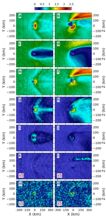
FIG. 2. 2D profiles of electric fields, normalized to vsw×
BIMF = 2.4 mV/m, along the plane through the cometary
nucleus and the direction parallel (left panels) and perpendic-ular (right panels) to the upstream interplanetary magnetic field. (a,b) Total electric field; (c,d) ion convective electric field; (e,f) electron convective electric field; (g,h) Hall electric field; (i,j) ambipolar electric field; (k,l) electron inertial term; (m,n) residual field. Note, the colors in panels k,l,m, and n are scaled by a factor 5 with respect to the other panels. The coordinate system is cometocentric with the +x direc-tion along the solar wind flow and the +y direcdirec-tion along the interplanetary magnetic field. With exception of panel m, the left-hand panels include also field lines representative of the magnetic topology.
4 convective electric field generated by the solar wind and
141
cometary electron species combined, and the residual 142
after subtracting the contributions from the electron 143
inertia and all right-hand side terms of Eq. 1 from the 144
total simulated electric field. Upstream and away from 145
the interaction region, the total electric field (panels a 146
and b) is dominated by the convective term generated by 147
the motion of the solar wind protons and the cometary 148
water ions in the comet frame (panels c and d). Closer 149
to the cometary nucleus the situation becomes more 150
complex. As the solar wind plasma becomes more and 151
more mass-loaded by cold cometary ions and the solar 152
wind protons are deflected perpendicular to the magnetic 153
field and away from the cometary nucleus [7, 48], the 154
ions decouple from the magnetic field while the electrons 155
remain frozen-in (panels e and f). The dark red shading 156
in the upper right corner of panel f corresponds to the 157
region where the cometary electrons are picked-up (see 158
also Fig. 1), creating an electron current that induces 159
the magnetic field pile-up upstream of the cometary 160
nucleus [14]. The difference between the ion and electron 161
convective electric fields is the Hall electric field (panels 162
g and h). 163
164
Two more significant regions are noticeable in the 165
total electric field: (1) an area where the electric field 166
magnitude strongly drops, corresponding to the location 167
upstream of the nucleus where the solar wind electrons 168
couple most effectively with the cometary ions, and 169
(2) a banana-shaped region just downstream of the 170
cometary nucleus where the Hall electric field is most 171
pronounced, serving to redirect the solar wind electrons 172
into following the cometary ions through their pick-173
up process. Both regions are most clearly seen in Fig. 2b. 174
175
In the regions where the electron pressure gradient 176
dominates a strong ambipolar electric field is present, 177
e.g., near the outgassing cometary nucleus [43, 44, 49]. 178
Here the electric field can do work and accelerate elec-179
trons parallel to the magnetic field towards the comet 180
(panels i and j). Hence, providing further evidence that 181
the ambipolar electric field generates the suprathermal 182
electron population close to the comet [7, 43, 44]. 183
Note that the analysis presented here cannot exclude 184
an extra electron acceleration source through lower-185
hybrid-waves [50]. In addition, in the perpendicular 186
direction (panel j) a symmetric structure is not expected 187
because of the near-comet cross-field acceleration, i.e., 188
the beginning of the pick-up process. 189
190
We find that the role of the electron inertia in the 191
time-averaged electric field (me
e ∇ · (ueue), neglected
192
in Eq. 1) has a negligible contribution in the balance 193
of the total electric field close to the cometary nucleus 194
(panel k). On the other hand, it may play a limited 195
role at the inner edge of the region where the solar wind 196
ions are deflected (panel l). Splitting up the pressure 197
tensor in its diagonal and non-diagonal components 198
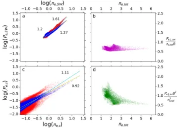
FIG. 3. Electron pressures in the near-cometary environment as a function of the electron number density for (a) the solar wind and (c) the cometary electrons. (b,d) The adiabatic in-variants calculated in a 50 km radius around the nucleus [3] as a function of the electron number density. Note that this radius has been selected empirically in order to most clearly show the influence of the cometary interaction. Each dot in the scatter plots represents one computational cell. The paral-lel electron pressure is colored red, the perpendicular electron pressure blue. The slope of the best linear fit through the respective population is indicated as well using the comple-mentary color.
(not shown here), the non-diagonal contribution to the 199
electron pressure tensor (i.e., the electron gyroviscosity, 200
typically described by an artificial viscous term in 201
electron fluid models) is entirely localized downstream of 202
the comet and bound to the XZ-plane perpendicular to 203
the magnetic field. This narrow area corresponds to the 204
region of space characterized by strong electron velocity 205
shears. 206
207
Finally, evaluating the residual electric field, no 208
structures above the simulation noise level are present 209
(panels m and n), confirming that the assumptions made 210
to derive the GOL are valid at the comet, at least at the 211
assumed spatial and frequency scales. Note that in case 212
a realistic ion-electron mass ratio is adopted, the residual 213
component would be even smaller. Hence, the observed 214
(already negligible) contribution can be considered an 215
upper limit. The GOL constructed here describes well 216
the physical processes and the electron dynamics at play 217
in the solar wind interaction with a weakly outgassing 218
comet at steady-state. Note that the further away from 219
the cometary nucleus, and hence from the region where 220
electron kinetics dominates, the better the classic GOL 221
approximation becomes. This justifies, as expected, the 222
use of reduced models for large scale descriptions. 223
224
Now that the validity of the GOL (Eq. 1) has been 225
verified using self-consistent fully kinetic simulations, 226
we concentrate on the only remaining term that carries 227
information on the electron kinetic evolution through 228
the properties of the electron pressure tensor, namely 229
the ambipolar electric field. In particular, we look for 230
a simple equivalent polytropic closure in the cometary 231
environment that could mimic the mixed cometary and 232
solar wind electron behavior (Fig. 3). We find that the 233
cometary electrons exhibit an apparent isotropic and 234
almost isothermal behavior. The latter is a signature of 235
the steady-state ionization of the expanding cometary 236
ionosphere that creates charged particles character-237
ized by the same initial averaged energy (assumed in 238
the model). The solar wind electrons, on the other 239
hand, exhibit an anisotropic and apparent polytropic 240
behavior. The perpendicular polytropic index measures 241
γe,⊥ ' 1.27, while the parallel polytropic index reveals
242
a knee close to the value of the upstream solar wind 243
density (n ' 1 km s−1), where γe,k ' 1.2 (resp. 1.62) at
244
lower (resp. higher) densities, implying an electron pres-245
sure anisotropy. Note that to have different adiabatic 246
indexes between parallel and perpendicular pressures 247
implies the generation of pressure anisotropies through 248
compression/depression, which are themselves a source 249
of free energy for plasma instabilities to develop. The 250
deviation from polytropic behavior concentrates in the 251
inner coma region (cometary ionosphere). It can be well 252
described by a double adiabatic compression [3] of the 253
perpendicular pressure (Fig. 3b). The parallel electron 254
pressure is not adiabatic (Fig. 3d) as a consequence of 255
the parallel electron acceleration in the close plasma 256
environment of a comet [7, 49]. 257
258
The above considerations need to be included for 259
an accurate representation of Πe when constructing a
260
GOL for a more restrictive computational approach. 261
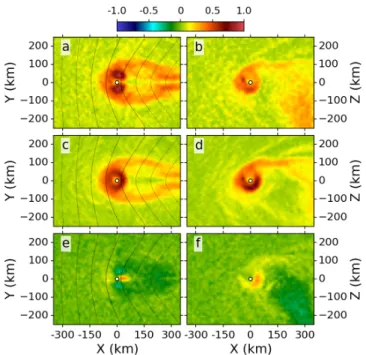
Fig 4 quantifies the error made (panels e and f) when 262
characterizing the electron pressure tensor by a single 263
temperature (panels c and d, here computed using the 264
trace of Πe), or in other words, by neglecting both
265
the off-diagonal and parallel/perpendicular information 266
of the two simulated electron species. Panels a and b 267
correspond to panels i and j in Fig. 2. Near the nucleus, 268
i.e., in the electron trapping region that is responsible 269
for the generation of the suprathermal electron distribu-270
tions [7, 22, 49], panels (e,f) reveal differences up to 50% 271
between the full and simplified electron pressure tensor. 272
This is particularly prevalent downstream of the nucleus 273
where the cometary electron pick-up process dominates. 274
The correct representation of the ambipolar electric field 275
is crucial for electron acceleration [43, 44] and, hence, 276
not doing so might result in a misleading description of 277
the electron dynamics. 278
279
Interestingly, Giotto electron and magnetic field 280
measurements from its flyby of comet 1P/Halley [51, 52] 281
showed a similar perpendicular polytropic index 282
(γ⊥ ∼ 1.3). A significantly smaller value was found,
283
however, for the parallel one (γk ∼ 0.55), indicative
284
of a more efficient electron cooling mechanism dur-285
FIG. 4. 2D profiles of the ambipolar electric field, normal-ized to vsw× BIMF= 2.4 mV/m, along the plane through the
cometary nucleus and the direction parallel (left panels) and perpendicular (right panels) to the upstream interplanetary magnetic field. (a,b) Ambipolar electric field computed using the total electron pressure tensor, corresponding to panels i and j in Fig. 2; (c,d) ambipolar electric field computed using the trace of the total electron pressure tensor; (e,f) difference between the panels above (c minus a,d minus b). The coordi-nate system is cometocentric with the +x direction along the solar wind flow and the +y direction along the interplanetary magnetic field. The left-hand panels include also field lines representative of the magnetic topology.
ing wave compression. Note that these observations 286
correspond to suprathermal electrons with energies 287
ranging from 30 to 80 eV, while the mean solar wind and 288
cometary electron energy measured approximately 10 eV. 289
290
To conclude, in this letter we have simulated the 291
solar wind interaction with a weakly outgassing comet 292
and computed the terms of a GOL directly from the 293
complete electron dynamics of the simulation. The 294
relative importance of each of these terms has allowed us 295
to isolate the driving physics in the various regions of the 296
cometary plasma environment, rather than assuming it. 297
We find that close to the outgassing nucleus the electron 298
pressure gradient dominates, and that at sub-ion scales 299
the total electric field is a superposition of the solar 300
wind convective electric field and the ambipolar electric 301
field. The contributions to the electric field from the 302
electron inertia and mass-loading of the solar wind are 303
both negligible. Most importantly, we have shown for a 304
weakly outgassing object that a GOL and the associated 305
electron equation of motion can be applied as long as 306
the full electron pressure tensor is considered to describe 307
6 the complex electron dynamics of a multi-species plasma
308
environment. 309
310
The comparison of our simulations with the limitation 311
of a GOL approximation and the derived polytropic in-312
dices deliver compelling information for a wide range of 313
modelling approaches where a self-consistent treatment 314
of the electron dynamics is unfeasible. By averaging the 315
simulation output over time, we have effectively removed 316
wave dynamics and, hence, the polytropic indices de-317
duced here provide an effective electron closure at low 318 frequencies. 319 320 ACKNOWLEDGMENTS 321
This work was supported in part by NASAs So-322
lar System Exploration Research Virtual Institute 323
(SSERVI): Institute for Modeling Plasmas, Atmo-324
sphere, and Cosmic Dust (IMPACT), and the NASA 325
High-End Computing (HEC) Program through the 326
NASA Advanced Supercomputing (NAS) Division at 327
Ames Research Center. We acknowledge PRACE for 328
awarding us access to Curie at GENCI@CEA, France. 329
Test simulations were performed at the Lomonosov 330
supercomputing facility (Moscow State University) 331
under projects nr. 1576 and 1658. Part of this work was 332
inspired by discussions within International Team 402: 333
Plasma Environment of Comet 67P after Rosetta at the 334
International Space Science Institute, Bern, Switzerland. 335
Work at LPC2E/CNRS was supported by CNES and by 336
ANR under the financial agreement ANR-15-CE31-0009-337
01. Partial support is also acknowledged by Contract 338
No. JPL-1502225 at the University of Colorado from 339
Rosetta, which is an European Space Agency (ESA) 340
mission with contributions from its member states and 341
NASA. Work at Imperial College London is supported 342
by STFC of UK under grant ST/N000692/1 and ESA 343
under contract No.4000119035/16/ES/JD. 344
345
[1] S. A. Ledvina, Y.-J. Ma, and E. Kallio, Space Science Reviews 139, 143 (2008).
[2] F. Valentini, P. Tr´avn´ıˇcek, F. Califano, P. Hellinger, and A. Mangeney, Journal of Computational Physics 225, 753 (2007).
[3] G. F. Chew, M. L. Goldberger, and F. E. Low, Proceed-ings of the Royal Society A: Mathematical, Physical and Engineering Sciences 236, 112 (1956).
[4] T. Chust and G. Belmont, Physics of Plasmas 13, 012506 (2006).
[5] K. Szeg˝o, K.-H. Glassmeier, R. Bingham, A. Bogdanov, C. Fischer, G. Haerendel, A. Brinca, T. Cravens, E. Du-binin, K. Sauer, L. Fisk, T. Gombosi, N. Schwadron, P. Isenberg, M. Lee, C. Mazelle, E. M¨obius, U. Motschmann, V. D. Shapiro, B. Tsurutani, and G. Zank, Space Science Reviews 94, 429 (2000). [6] T. I. Gombosi, in Magnetotails in the Solar System,
Washington DC American Geophysical Union Geophys-ical Monograph Series, Vol. 207, edited by A. Keiling, C. M. Jackman, and P. A. Delamere (2015) pp. 169– 188.
[7] J. Deca, A. Divin, P. Henri, A. Eriksson, S. Markidis, V. Olshevsky, and M. Hor´anyi, Physical Review Letters 118, 205101 (2017).
[8] K.-H. Glassmeier, H. Boehnhardt, D. Koschny, E. K¨uhrt, and I. Richter, Space Science Reviews 128, 1 (2007). [9] M. G. G. T. Taylor, N. Altobelli, B. J. Buratti, and
M. Choukroun, Philosophical Transactions of the Royal Society of London Series A 375, 20160262 (2017), arXiv:1703.10462 [astro-ph.EP].
[10] G. Clark, T. W. Broiles, J. L. Burch, G. A. Collinson, T. Cravens, R. A. Frahm, J. Goldstein, R. Goldstein, K. Mandt, P. Mokashi, M. Samara, and C. J. Pollock, Astronomy & Astrophysics 583, A24 (2015).
[11] L. Yang, J. J. P. Paulsson, C. S. Wedlund, E. Odelstad, N. J. T. Edberg, C. Koenders, A. I. Eriksson, and W. J.
Miloch, Monthly Notices of the Royal Astronomical So-ciety 462, S33 (2016).
[12] M. R. Combi and P. D. Feldman, Icarus 105, 557 (1993). [13] C. Snodgrass, C. Tubiana, D. M. Bramich, K. Meech, H. Boehnhardt, and L. Barrera, Astronomy & Astro-physics 557, A33 (2013), arXiv:1307.7978 [astro-ph.EP]. [14] H. Nilsson, G. Stenberg Wieser, E. Behar, C. Simon Wed-lund, E. Kallio, H. Gunell, N. J. T. Edberg, A. I. Eriks-son, M. Yamauchi, C. Koenders, and et al., Astronomy & Astrophysics 583, A20 (2015).
[15] C. Simon Wedlund, E. Kallio, M. Alho, H. Nilsson, G. Stenberg Wieser, H. Gunell, E. Behar, J. Pusa, and G. Gronoff, Astronomy & Astrophysics 587, A154 (2016).
[16] C. S. Wedlund, M. Alho, G. Gronoff, E. Kallio, H. Gunell, H. Nilsson, J. Lindkvist, E. Behar, G. S. Wieser, and W. J. Miloch, Astronomy & Astrophysics 604, A73 (2017).
[17] C. Simon Wedlund, E. Behar, H. Nilsson, M. Alho, E. Kallio, H. Gunell, D. Bodewits, K. Heritier, M. Ga-land, A. Beth, and et al., Astronomy & Astrophysics (2019), 10.1051/0004-6361/201834881.
[18] K. Heritier, M. Galand, P. Henri, F. Johansson, A. Beth, A. Eriksson, X. Valli`eres, K. Altwegg, J. Burch, C. Carr, et al., Astronomy & Astrophysics 618, A77 (2018). [19] N. J. T. Edberg, A. I. Eriksson, E. Odelstad, P. Henri,
J.-P. Lebreton, S. Gasc, M. Rubin, M. Andr´e, R. Gill, E. P. G. Johansson, F. Johansson, E. Vigren, J. E. Wahlund, C. M. Carr, E. Cupido, K.-H. Glassmeier, R. Goldstein, C. Koenders, K. Mandt, Z. Nemeth, H. Nilsson, I. Richter, G. S. Wieser, K. Szego, and M. Volwerk, Geophysical Research Letters 42, 4263 (2015).
[20] K. Heritier, P. Henri, X. Valli`eres, M. Galand, E. Odel-stad, A. Eriksson, F. Johansson, K. Altwegg, E. Behar, A. Beth, et al., Monthly Notices of the Royal
Astronom-ical Society 469, S118 (2017).
[21] H. Nilsson, G. S. Wieser, E. Behar, H. Gunell, M. Wieser, M. Galand, C. Simon Wedlund, M. Alho, C. Goetz, M. Yamauchi, P. Henri, E. Odelstad, and E. Vigren, Monthly Notices of the Royal Astronomical Society 469, S252 (2017).
[22] A. I. Eriksson, I. A. D. Engelhardt, M. Andr´e, R. Bostr¨om, N. J. T. Edberg, F. L. Johansson, E. Odel-stad, E. Vigren, J.-E. Wahlund, P. Henri, J.-P. Lebre-ton, W. J. Miloch, J. J. P. Paulsson, C. Simon Wedlund, L. Yang, T. Karlsson, R. Jarvinen, T. Broiles, K. Mandt, C. M. Carr, M. Galand, H. Nilsson, and C. Norberg, Astronomy & Astrophysics 605, A15 (2017).
[23] L. Berˇciˇc, E. Behar, H. Nilsson, G. Nicolaou, G. S. Wieser, M. Wieser, and C. Goetz, Astronomy & As-trophysics 613, A57 (2018).
[24] Y. D. Jia, M. R. Combi, K. C. Hansen, T. I. Gombosi, F. J. Crary, and D. T. Young, Icarus 196, 249 (2008). [25] M. Rubin, C. Koenders, K. Altwegg, M. R. Combi,
K.-H. Glassmeier, T. I. Gombosi, K. C. Hansen, U. Motschmann, I. Richter, V. M. Tenishev, and G. T´oth, Icarus 242, 38 (2014).
[26] M. Rubin, M. R. Combi, L. K. S. Daldorff, T. I. Gombosi, K. C. Hansen, Y. Shou, V. M. Tenishev, G. T´oth, B. van der Holst, and K. Altwegg, The Astrophysical Journal 781, 86 (2014).
[27] M. Rubin, T. I. Gombosi, K. C. Hansen, W.-H. Ip, M. D. Kartalev, C. Koenders, and G. T´oth, Earth Moon and Planets 116, 141 (2015).
[28] Z. Huang, G. T´oth, T. I. Gombosi, X. Jia, M. Rubin, N. Fougere, V. Tenishev, M. R. Combi, A. Bieler, K. C. Hansen, Y. Shou, and K. Altwegg, Journal of Geophys-ical Research (Space Physics) 121, 4247 (2016).
[29] Y. Shou, M. Combi, G. Toth, V. Tenishev, N. Fougere, X. Jia, M. Rubin, Z. Huang, K. Hansen, T. Gombosi, and A. Bieler, The Astrophysical Journal 833, 160 (2016). [30] N. Gortsas, U. Motschmann, E. K¨uhrt, J. Knollenberg,
S. Simon, and A. Boesswetter, Annales Geophysicae 27, 1555 (2009).
[31] S. Wiehle, U. Motschmann, N. Gortsas, K.-H. Glass-meier, J. M¨uller, and C. Koenders, Advances in Space Research 48, 1108 (2011).
[32] C. Koenders, K.-H. Glassmeier, I. Richter, U. Motschmann, and M. Rubin, Planetary and Space Science 87, 85 (2013).
[33] C. Koenders, K.-H. Glassmeier, I. Richter, H. Ranocha, and U. Motschmann, Planetary and Space Science 105, 101 (2015).
[34] E. Behar, J. Lindkvist, H. Nilsson, M. Holmstr¨om, G. Stenberg-Wieser, R. Ramstad, and C. G¨otz, Astron-omy & Astrophysics 596, A42 (2016).
[35] C. Koenders, C. Goetz, I. Richter, U. Motschmann, and K.-H. Glassmeier, Monthly Notices of the Royal Astro-nomical Society 462, S235 (2016).
[36] C. Koenders, C. Perschke, C. Goetz, I. Richter,
U. Motschmann, and K. H. Glassmeier, Astronomy & Astrophysics 594, A66 (2016).
[37] J. Lindkvist, M. Hamrin, H. Gunell, H. Nilsson, C. Si-mon Wedlund, E. Kallio, I. Mann, T. Pitk¨anen, and T. Karlsson, Astronomy & Astrophysics 616 (2018). [38] S. Markidis, G. Lapenta, and Rizwan-uddin,
Mathemat-ics and Computers in Simulation 80, 1509 (2010). [39] R. J. Mason, Journal of Computational Physics 41, 233
(1981).
[40] J. U. Brackbill and D. W. Forslund, Journal of Compu-tational Physics 46, 271 (1982).
[41] G. Lapenta, J. U. Brackbill, and P. Ricci, Physics of Plasmas 13, 055904 (2006).
[42] K. C. Hansen, K. Altwegg, J.-J. Berthelier, A. Bieler, N. Biver, D. Bockel´ee-Morvan, U. Calmonte, F. Capac-cioni, M. Combi, J. De Keyser, et al., Monthly Notices of the Royal Astronomical Society , stw2413 (2016). [43] A. Divin, J. Deca, A. Eriksson, P. Henri, G. Lapenta,
V. Olshevsky, and S. Markidis, Geophysical Research Letters (2019).
[44] C. Sishtla, A. Divin, J. Deca, V. Olshevsky, and S. Markidis, Physics of Plasmas (2019).
[45] I. Richter, C. Koenders, H.-U. Auster, D. Fr¨uhauff, C. G¨otz, P. Heinisch, C. Perschke, U. Motschmann, B. Stoll, K. Altwegg, J. Burch, C. Carr, E. Cupido, A. Eriksson, P. Henri, R. Goldstein, J.-P. Lebreton, P. Mokashi, Z. Nemeth, H. Nilsson, M. Rubin, K. Szeg¨o, B. T. Tsurutani, C. Vallat, M. Volwerk, and K.-H. Glass-meier, Annales Geophysicae 33, 1031 (2015).
[46] T. Karlsson, A. I. Eriksson, E. Odelstad, M. Andr´e, G. Dickeli, A. Kullen, P.-A. Lindqvist, H. Nilsson, and I. Richter, Geophysical Research Letters 44, 1641 (2017). [47] J. Deca, A. Divin, B. Lemb`ege, M. Hor´anyi, S. Markidis, and G. Lapenta, Journal of Geophysical Research: Space Physics , 6443 (2015), 2015JA021070.
[48] E. Behar, B. Tabone, M. Saillenfest, P. Henri, J. Deca, M. Holmstr¨om, and H., Astronomy & Astrophysics (2018), 10.1051/0004-6361/201832736.
[49] H. Madanian, T. E. Cravens, A. Rahmati, R. Goldstein, J. Burch, A. I. Eriksson, N. J. T. Edberg, P. Henri, K. Mandt, G. Clark, M. Rubin, T. Broiles, and N. L. Reedy, Journal of Geophysical Research (Space Physics) 121, 5815 (2016).
[50] T. W. Broiles, J. L. Burch, K. Chae, G. Clark, T. E. Cravens, A. Eriksson, S. A. Fuselier, R. A. Frahm, S. Gasc, R. Goldstein, P. Henri, C. Koenders, G. Livadi-otis, K. E. Mandt, P. Mokashi, Z. Nemeth, E. Odelstad, M. Rubin, and M. Samara, Monthly Notices of the Royal Astronomical Society 462, S312 (2016).
[51] G. Belmont and C. Mazelle, Journal of Geophysical Re-search 97, 8327 (1992).
[52] C. Mazelle and G. Belmont, Geophysical Research Let-ters 20, 157 (1993).