Variation of ground snow loads with elevation in southern British Columbia

(1)

Publisher’s version / Version de l'éditeur:

Canadian Journal of Civil Engineering, 11, September 3, pp. 480-493, 1984-09

READ THESE TERMS AND CONDITIONS CAREFULLY BEFORE USING THIS WEBSITE. https://nrc-publications.canada.ca/eng/copyright

Vous avez des questions? Nous pouvons vous aider. Pour communiquer directement avec un auteur, consultez la première page de la revue dans laquelle son article a été publié afin de trouver ses coordonnées. Si vous n’arrivez pas à les repérer, communiquez avec nous à PublicationsArchive-ArchivesPublications@nrc-cnrc.gc.ca.

Questions? Contact the NRC Publications Archive team at

PublicationsArchive-ArchivesPublications@nrc-cnrc.gc.ca. If you wish to email the authors directly, please see the first page of the publication for their contact information.

NRC Publications Archive

Archives des publications du CNRC

This publication could be one of several versions: author’s original, accepted manuscript or the publisher’s version. / La version de cette publication peut être l’une des suivantes : la version prépublication de l’auteur, la version acceptée du manuscrit ou la version de l’éditeur.

Access and use of this website and the material on it are subject to the Terms and Conditions set forth at

Variation of ground snow loads with elevation in southern British

Columbia

Claus, B. R.; Russell, S. O.; Schaerer, P. A.-W

https://publications-cnrc.canada.ca/fra/droits

L’accès à ce site Web et l’utilisation de son contenu sont assujettis aux conditions présentées dans le site LISEZ CES CONDITIONS ATTENTIVEMENT AVANT D’UTILISER CE SITE WEB.

NRC Publications Record / Notice d'Archives des publications de CNRC:

https://nrc-publications.canada.ca/eng/view/object/?id=db0b5042-f57b-41a9-9391-b94834f5c479 https://publications-cnrc.canada.ca/fra/voir/objet/?id=db0b5042-f57b-41a9-9391-b94834f5c479

(2)

National Research Conseil national

I

*

Council Canada de recherches Canada

VARIATION OF GROUND SNOW LOADS WITH ELEVATION IN SOUTHERN BRITISH COLUMBIA

ANALYZED

by B.R. Claus, S.O. Russell and P. Schaerer

I.ct:

-

N R C

-

C l S T l \I

_{BLDG RES.}

1, '1

L ~ R A R Y

'I,

!

i Reprinted from

Canadian Journal of Civil Engineering, Vol. 11 No. 3 1984

p. 480-493

I

DBR Paper No. 1217

vision of Building Research

Price $1.25 OTTAWA _{NRCC 23579}

(3)

This paper, while being distributed in reprint form by the Division of Building Research, remains the copyright of the original publisher. It should not be reproduced in whole or in part without the permission of the publisher.

A l ~ s t of all publications available from the Division may be

obtained by w r k n ~ to_thePublicatianS~cti~n~~vision of _.

Building 1

(4)

Variation of ground snow loads with elevation in Southern British Columbia

B. R. CLAUS

Sigma Engineering Ltd., 1155 West Georgia Street, Vancouver, B . C . , Canada V6E 3H4 S. 0. RUSSELL

Civil Engineering Department, University of British Columbia, Vancouver, B . C . , Canada V6T 1 W5 AND

P . SCHAERER

Division of Building Research, National Research Council of Canada, 3904 West 4th Avenue, Vancouver, B . C . , Canada V6R l P 5

Received May 10, 1983

Revised manuscript accepted April 3, 1984

Measurements conducted at 20 locations in Southern British Columbia were used to investigate the relationship between design ground snow load and elevation. It was found that the increase in water equivalent with elevation (i.e., the slope of the graph of water equivalent plotted against elevation) could be defined for regions having similar climatic conditions. For a given location, the design ground snow load can therefore be estimated by extrapolating from the water equivalent value at one elevation, where it has been meusured, to the elevation at the location in question.

Plots of the absolute values of water equivalents against elevation for regions of similar climatic conditions gave less satisfactory relationships but they could still be used to estimate approximate values of the design ground snow loads for any particular site.

La relation entre la charge nominale de neige au sol et I'altitude a CtC CtudiCe avec les observations de 20 postes de mesure situCs dans le sud de la Colombie Britannique. I1 a CtC trouvC que l'augmentation de 1'Cquivalent en eau en fonction de I'altitude (i.e. la pente de la courbe de ]'equivalent en eau en fonction de I'altitude) peut Ctre dCfinie pour des regions dont les conditions climatiques sont semblables. En un endroit donnC, la charge nominale de neige au sol peut donc Ctre estimCe par extrapolation connaissant la valeur de 1'Cquivalent en eau, l'altitude du point ou I'observation a CtC faite et l'altitude de I'endroit considCre. Les relations entre la valeur absolue de 1'Cquivalent en eau et l'altitude, pour des regions dont les conditions climatiques sont semblables, se sont avCrCes moins bonnes mais elles pourraient Ctre utilisCes pour approximer les charges nominales de neige au sol a n'importe quel endroit d o n d .

[Traduit par la revue] Can. J. Civ. Eng. 11, 480-493 (1984)

Introduction studies have been by Schaerer (1970) and Claus (1981, The determination of snow loads for the design of 1983). This Paper Presents a and a buildings generally involves two steps. First a design tinuation this

value for the ground snow load is estimated, and then the ground snow load is converted to a roof load, taking into account such factors as wind, roof height, and roof shape (Associate Committee on the National Building Code 1980a,b). Design ground snow loads depend on the return period chosen, the elevation, and the climatic region (Salm 1977).

For most locations in Canada, design snow depths have been determined from frequency analyses of measured maximum annual snow depths, using the Gumbel distribution to derive the 30 year return period value. These values were then converted to snow loads using an assumed snow density and making an adjustment to include the effects of rainfall (Taylor 1980).

Few studies have concerned themselves directly with the effects of elevation on the ground snow loads as applied to roof loadings. In British Columbia the only

Major climatic regions of Southern British Columbia

The climate of southern British Columbia varies con- siderably as one travels from west to east. On a regional basis, the climate is largely determined by the large- scale topography and the proximity of the Pacific Ocean. Northwest- southeast trending mountain ranges present a barrier, to the moisture-rich prevailing westerly winds. As the maritime air moves inland and is forced by the mountain barriers to rise, precipitation is released, and the air becomes progressively drier as it passes successive ranges.

On a smaller scale, climatic conditions are modified by local physiographic factors such as slope, elevation, and aspect. The rising air generally releases much more precipitation on the western sides of mountain ranges

(5)

CLAUS ET AL. _{48 1}

than on the drier leeward sides.

The major climatic regions of Southern British Columbia can be very broadly classified as follows (Chapman 1952; Kendrew and Kerr 1955):

The coast mountains of B.C. are characterized by mildness, humidity, and extremely heavy precipitation especially in the mountains. Snowfall is generally limited to higher elevations, and snowpacks that accumu- late generally develop high densities because of rainfall and warm temperatures during the winter.

The southwest interior region, bordered by the Coast Range to the west and the Columbia Mountains to the east, is a region of continental climate, its arid characteristics resulting from the rain shadow effect of the Coast Range.

The southeast interior and southern Rockies region is very mountainous, and as such has higher precipitation than the dry interior, especially on the west-facing slopes, although the valleys are semiarid. Because of the higher elevations, temperatures are lower, and about one-half of the annual precipitation falls as snow.

I

Measurements

Locations

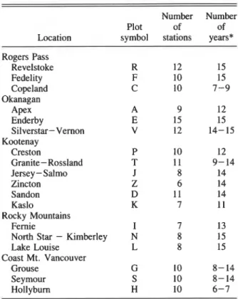
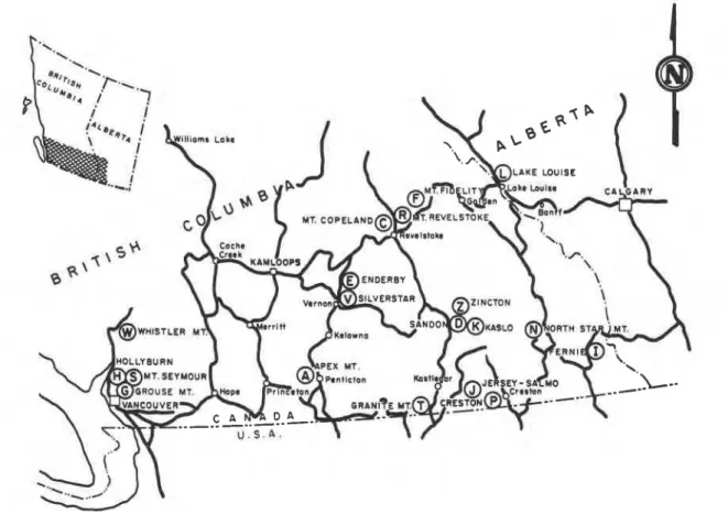
In 1965 the National Research Council of Canada initiated a program to measure snow water equivalents over a range of elevations in British Columbia. A number of mountainous areas throughout southern British Columbia were selected as locations for the measurements. These were generally near centers of popu- lation where there is need for snow load information. Of prime importance was accessibility in the winter by truck or snowmobile. The mountain locations, the number of measurement stations on each mountain, and the approximate number of years of observation are given in Table 1. The locations are shown in Fig. 1.

Each mountain location had from 6 to 15 measurement stations spaced at elevation intervals of between 100 and 150 m. A typical station would be in a small clearing of approximately two tree heights in width. An attempt was made to find stations that were as wind free as possible, had similar aspect and vegeta- tion, and were representative of their areas.

I

I Data collection

I

Collection of data was started by the National Re- search Council in 1967, with the number of stations increasing in subsequent years. Most of the measurements were taken by National Research Council staff.

Snow depth and water equivalents were measured at each station. The water equivalent measurements were made with a Federal snow sampler with approximately three measurements made per station. Although more measurements at each station would have been de-

TABLE 1. Snow measurements locations

Number Number Plot of of Location symbol stations years* Rogers Pass Revelstoke Fedelity Copeland Okanagan Apex Enderby Silverstar-Vernon Kootenay Creston Granite- Rossland Jersey - Salmo Zincton Sandon Kaslo Rocky Mountains Fernie

North Star - Kimberley Lake Louise

Coast Mt. Vancouver Grouse

Seymour Holl yburn

sirable. it was felt that three careful measurements done at many stations were preferable to a larger number of measurements at a smaller number of stations. Tests have shown that the Federal snow sarn~ler over- measures water equivalents by between 6 and 12%. In line with standard practice, these were corrected by multiplying the readings by 0.92 (Schaerer 1970).

Since only the annual maximum water equivalents were of interest, measurements were taken at approximately 2 week intervals during the period when the maximum values were expected. Although the maximum snow depth may be missed because of snow settlement, water equivalents generally do not decrease until spring melting occurs. Only in the Vancouver area, where temperatures are much warmer and melting can begin immediately, did the measurements have to be taken right after a snowfall. Generally, maximum values occurred in the valleys in January or February whereas at higher elevations, maximum values were recorded later, generally in April or May.

Analysis Choice of distribution

At each measurement station, statistical parameters such as mean, standard deviation, and coefficient of variation of the annual maximum water equivalents

(6)

CAN. I. CIV. ENG. VOL. 11. 1984

FIG. 1. Location of snow measuring stations. were calculated.

An extreme-value distribution was then used to cal- culate the expected 30 year return maximum water equivalent. A 30 year return period was chosen because this is the return period presently being used for the design of buildings in Canada. In detailed analysis, it could be reasonable to specify different return periods for different uses, for example farm buildings versus buildings for human habitation.

Four common distributions, the Gumbel, normal, lognormal, and cube root normal distributions, were used and the results were compared. In calculating the

30 year values, the student-t distribution was used for

the latter three normal-based distributions to adjust for the actual number of years of observations. For example, with the cube root normal distribution, the cube roots of the annual maximum water equivalents were assumed to have a student-t distribution rather than a normal distribution. Both distributions give the same results when there are many data points, but the fewer the number of data points, the more conservative the 30 year value estimated on the basis for the student-t distribution. Formulae and tables are given in Benjamin and Come11 (1970).

The 30 year return maximum water equivalents ob- tained from the different distributions gave similar values, with the exception of the lognormal distribution, which produced anomalous values when the measured water equivalents were near zero. Since the cube root normal distribution produced results similar to those from the other distributions, allowed inclusion of the effects of sample size through use of the student-t distribution, and is widely used in the analysis of climatic data by government agencies in British Col- umbia, it was used in the analysis. As more years of data become available, the Gumbel distribution may become more suitable and perhaps preferable because of its widespread acceptance in hydrological work.

Regression analyses

The calculated 30 year maximum water equivalents and the computed means and standard deviations of the measured annual maximum values were plotted against elevation for each individual mountain location. Least squares regression analyses were performed, and for each case, the degree of fit r2 was determined, where r is the correlation coefficient.

(7)

CLAUS ET AL. 483

TABLE 2. Regression coefficients for water equivalent

-

elevation relationship Water equivalent (mm) = A

+

B(e1evation)

+

C(e1evation)'

Region A B C r Z N Rogers Pass (R, F) Okanagan (A, E, V) Kootenay (P, T, J, Z, S, K) South Kootenay (P, T, J) North Kootenay (Z, D, K) Interior average (R, F, A, E, V, P, T, J, Z, D, K) Rocky Mt. Dry (N, L) Coast Mt. Vancouver (G, S, H)

NOTES: 30 year return maximum water equivalents in millimetres. Elevations in metres. N refers to number of stations and location codes (see Table 1 for explanation) are given in parentheses. This table is best used in conjunction with plots of data with the regression curve to check applicability for a given elevation.

statistical values was not intended to be directly representative of a physical cause, but rather to define empir- ical relationships. Linear and quadratic curves have been reported in the literature, and in Switzerland, a quadratic relationship is used to specify design snow loads (Zingg 1968). Quadratic regression curves gave relatively high degrees of fit and in a few trial cases these were much better than those from linear regression (Claus 1981). In the present study, therefore, quadratic regression curves have been used throughout.

Regions with similar ground snow load characteristics

Parameters used to identify regions

Regional areas with similar snow accumulation characteristics were defined on the basis of plotted relationships, trial calculations, and geographical proximity. This allows data from a few stations to be extrapolated to a larger area. Initially, it was hoped to obtain relationships between elevation and both the mean annual maximum water eauivalent and its stan-

cations were therefore grouped into regions based on analyses of the 30 year values. These groupings are given in Table 2 together with the constants derived for use in the regression equations for each group. The relationships are plotted in Figs. 2- 5.

Increase in snow load with elevation

When plots of the 30 year maximum water equivalent vs. elevation from various locations within a larger region were compared, they showed similar increases in water equivalents with elevation or similar "slope and curvature." When compared on a light table, the curves could be superimposed on one another by shifting the axes.

To quantify this relationship between the increase in water equivalent and elevation, additional least squares regression equations were derived where, this time, the "constant" term in the quadratic equation was allowed to vary and thus be dependent on the mountain location measured. These equations have the form

- -

dard deviation. From these two relationships, it would

where is the water equivalent; is the elevation; b , have been possible to determine the maximum water

are parameters, determined by regression analyses; equivalent at any elevation within the region for any

Z(s) is a dummy variable, Z(s) = 1 for location s, Z(s) return period. Quadratic least squares regression curves ₌

0 otherwise; and a ( s ) is the constant term for moun- for the mean annual maximum water equivalents fitted

tain location s. the combined data from several locations very well and

These analyses allowed larger regions to be defined r2 values above 0.95 were not uncommon. However, it

with increases in water equivalents with proved much more difficult to obtain quantitative trends

elevation. These regions are given in Table and he for groups of locations that defined standard deviations

relationships are plotted in Figs. 6 and 7. It is note- or other statistical parameters with acceptable accuracy.

w o ~ h y the Interior region has very similar in- Plots of the calculated 30 year maximum water

creases of water equivalent with elevation over a very equivalents against elevation showed an excellent fit to

large area. the regression curves. Since the 30 year maximum

water equivalents are of principal interest for design, it Discussion of water equivalent values for the regions was decided to work with these directly rather than with Some of the water equivalent - elevation curves for the component statistical parameters. Measurement lo- the different regions have distinct characteristics. For

(8)

- - . -

CAN. J. CIV. ENG. VOL. 1 1 , 1984

'JJUJOWS 00Qb OOZP 009E 000E OW1 0081 OOZI 009

a H Q 1 RQNS

-

lN3ltlAIn03 kJ3ltJM

n -1 0 O W -1

-

0 u = LL. W A

a

a> ' = m . w = El A rr &I- W I C1 = -1 z I- w=- L

-,

-

= L L a U

-

O . L L . o W m i

'

*

-

=+: % F B = E U U U1 U Z _U

2 -

-k- = W * L ? m u I F u =

-

_z

= =,'-N> J 0

=

_{* z} cym

-

w E

x z

I m ' b

-

L

*"

U) I Bb 3 9E OE bZ 8 1 ZT 9 u-l in I

-

c3

(9)

CLAUS ET AL.

CUCUO09E OOZE 0081 OW1 0001 0091 0021 008 OOb

C l t i O l MONS

-

l N 3 l t J A l f l D 3 d31tJM

CUCUO09E OOZE 0081 OOPZ 0002 0091 00ZL 008 OOb

(10)

486 CAN. J. CIV. ENG. VOL. 11, 1984

-

Z

2

a W n

2 $:

gap. C1 '2 Q N d 0

.-

_M 8

-

-0

-

E 8

%

r o w ?

??

+. m o w J x 03OUS m Z & o o U ,

cr

-

Z L , l l , , , l .

+ v, v, Z

G

5z2,mEI

-

a

-

ed4 ZE BZ PZ 02. 91 Z 1 8 tr r

- >

s

w -0

B

- W c 0 .- M

B

V) 2 a V) - 0 cr; wu009E OOZE 0082 O W 2 OOOZ 0091 002.1 008 O O b

-

u

aUO1 MONS

-

l N l l U A I f l 0 3 831UM

2 LI ,

-

Z a 7 w CJ L C ) O W cr x

?&

_0m-T or?

2

+

2:86!

xm?=?-- a m,oo I

-

b- w

-

0

-

ed)t 2E BZ tZ 02 91 ZT 8 P 1 a

3

E 0

.

C )

-

d

-

0 8 0 C 0 0 N

'ti

5

0 I C )

3 -2

.-

-

5 U E

s

_C 9

g

B

-0- -I- 3

cr

3 ' Z

4 J - w P L L 0 uuOD9E 00ZE 0082 O W 1 OOOZ 0091 0011 008 O@

(11)

WATER E Q U I V A L E N T

-

SNOW LOAD

400 800 1200 1600 2000 2400 2800 3200 3600mm

WATER E Q U I V A L E N T

-

SNOW

LOAD

400 800 1200 1600 2000 2400 2800 32011 3600mm 00 4 8 12 16 20 24 28 32 kPa + Ln l 004",

5

m c

.

OOOLD X . r n - OLD wUIm + E: w 4 - w o r n 0 r'l m-

5:

'

4 - w-

-

4 '-11 4 m ;D Z k r'l

-

(12)

CAN. I. CIV. ENG. VOL. 1 1 , 1984

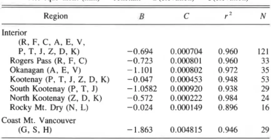
TABLE 3. Regression coefficients for relative water equivalent - elevation relationships

Water equivalent (mm) = constant

+

B(e1evation)

+

elevation)^

Region B C r N Interior (R, F, C, A, E, V, P, T, J , Z, D, K) Rogers Pass (R, F, C) Okanagan (A, E, V ) Kootenay (P, T, J, Z, D, K) South Kootenay (P, T, J) North Kootenay (Z, D, K) Rocky Mt. Dry (N, L) Coast Mt. Vancouver ( G , S, H)

NOTES: 30 year return maximum relative water equivalents in millimetres. Elevations in metres. N refers to number of stations and location codes (see Table 1 for explanation) are given in parentheses. Constants to be determined by substituting known maximum water equivalent values. This table is best used in conjunction with plots of data with the regression curve to check applicability for a given elevation.

example, magnitudes of water equivalents for the wetter regions, generally located on the windward sides of mountain ranges (e. g

.

, Vancouver region, Fernie) ,

increase very rapidly with elevation, and have some of the highest values in the province. A profile across southern British Columbia showing the topography and the snow water equivalents is given in Fig. 8. This illustrates the relation between elevation and water equivalents, as determined from the regional curves in this study.

The water equivalents of the colder regions (Kimberley, Lake Louise) have much lower values, and increase almost linearly with elevation and at much lower rates than the wet climate values. The "intermediate" climates in the southern interior of the province (Okanagan, Kootenays, and Rogers Pass region) have water equivalent values and rates of increase that are in between those of the wet and the dry regions. There are also significant local effects. An example is Mount Copeland, which, although close to Revelstoke and Rogers Pass in distance, has a very different water equivalent - elevation relationship.

The differences between the curves for the wet and the dry regions is probably due to different physical processes of snow accumulation. In wet climates, the increase in water equivalent with elevation is partly due to increased precipitation resulting from orographic effects and partly due to the effect of varying freezing levels. Freezing levels are often part way between mountain top and bottom elevations. During a storm, snow accumulates at elevations above the freezing level but not below it. In the drier colder climates, freezing levels are lower and the increase in water equivalent is

partly due to the increase in precipitation with elevation and partly to the longer accumulation period resulting from the lower temperatures at high elevations.

For both the South Coast Vancouver region and the Okanagan region, the relationship between snow water equivalent and elevation, as shown in Figs. 2 6 and 3b, is somewhat indeterminate below an elevation of 500 m. This is probably because there is no permanent snow below 500 m and the maximum accumulations are determined largely by individual snowfall events, while above 500 m snow that falls remains for most of the winter. The regression curves do not apply at these lower elevations.

In the calculation of roof loads using the present National Building Code, recommended ground snow loads are determined from the Table of Climatic Infor- mation in the Supplement of the National Building Code (Associate Committee on the National Building Code 1980b). A comparison of these values with the ground snow loads obtained in the present study is given in Table 4. Values were obtained from regional plots if measurements were not available close to the towns listed in the Table of Climatic Information in the Building Code. Some towns could not reliably be placed within the defined regions and no comparison could be made.

Table 4 shows generally close agreement between the values obtained from this study and those of the Nation- al Building Code (N.B .C.), although some values are up to 50% higher than the N.B .C. values and one at Penticton is almost 100% higher. These differences are probably due to three causes. Firstly, the N.B.C. measurements were not taken at exactly the same locations

(13)

-

- E m E m

2 %

:

!&

S 0

-

0 -

-

a

-

I- (a)COFIST VRNCI3UVER I- Z Z

a

_REGION

a

'-0 + O m - ?

Y g

CONST.

+

EX + CXX

₃

Q N = 29 Q 0 RSO = 0.946 0 C = 0.00481W 1 0 lo B = -1 .Hi324405

' i L - f i

- 0 . _(D m m _N _CONST. _LOCRTION N 0 10 325.36 61

a

Q 10 322.07 62 Q - w ( b ) l N T E R J O R REGION CONST. t BX t CXX N = J2J RSO = 0 -960 C = 0.00070416 B = -0.69345213 N CONST. LOCRTION 13 854.72 11 10 691.36 12 9 229.81 64 -'=:_-5", ₈10 1834.91 13 _{150.45 21} 3

2

15 288.60 22 Q Q Z 12 230.75 23

z

₁₀ _{601.26 31} C" _o ₁₁ _{550.51 32} I

= - - 2

-

8 4 1 2 . 3 4 3 3 N 6 525.06 41 I- I- 11 474.53 42 z 7 758.51 43 Z H W 3 3 0 W 0 1Y.

B

--

₌

W W I- I- CI c CT I I I I 0 2 1000 2000 0 1000 2000

E L E V A T I O N

(ml

E L E V A T I O N

(ml

(14)

(a) OKANAGAN

REGJDN

CONST.

+

9 X

+

CXX N CONST. L O C R T I O N

(b)

KOCtTENRY

REGJDN

CONST.

+

5X

+

CXX N 53 RSO = 13.948 N CONST. L O C R T I O N 10 230.30 31 11 181.93 32 8 88.16 33 G 7-71 -27 ₄₁ 11 109.76 42 E n E 3

E:

5

%

s

- c a Kt 0 , N - I- Z

a

' - 0

g g -

0 0 I

-8--nJ

N o

a

0 ,N- I- Z

a

. e r r ' - 0

z g -

Q 0 e I - z - - N N n a Q

- J g - - g

3

=

0 Z ' " 0 0

I 5

I- Z W *

A o - - Z

>"

-

fi

3 Q 3

E

0 Z

-- E

"

0 0

.-

'D,

'

5

I- Z W 0

J O - - Z

cc

> 2

M 3

a

(3 W g - - m W = : - - m E r n

w

W W I- I- a

a

' ? - - - a

3 p . t

W W

>

> CI CI I- I-

a

--

-I c3 W O [r: D 1000 2000 C) 1000 2000

ELEVRT

_I

ON

(m 1

ELEVRT

I

ON

(ml

(15)

CLAUS ET AL.

30 year max.

i

water equivalent mean annual max.-( water equivalent

Distance from Coast ( km

1 I

FIG. 8. East-west profile of British Columbia.

TABLE 4. Comparison between snow loads listed in Table of Climate Information of the National Building Code and the

present study

Ground Ground loads loads using using Elevation N.B.C. this study

Location (m) Coast- Vancouver North Vancouver 200 2.2 3.0 Okanagan Penticton Kelowna Vernon Rogers Pass Revelstoke Glacier Kootenay Kaslo Castlegar Crescent Valley Grand Forks Montrose Nakusp Nelson Trail Rocky Mt. Trench Kimberley Cranbrook Elko Fernie

as the measurements used in this study, and variations in local conditions can be expected to have a pro- nounced effect. Secondly, this study used a cube root normal probability distribution while the N .B .C. values are based on the Gumbel distribution. Lastly, the National Building Code snow loads were determined from snow depth data with an assumed snow density of

0 . 2 g/cc. For large snow depths, particularly in wetter

regions, this value may be too low and hence may give low ground snow load estimates (Claus 1981).

Determination of ground snow loads for design

The best method to determine ground snow loads for design is to use actual water equivalent or snow depth data if these are available. If no data are available for the site in question, the results of this study can be used as an aid to determine design ground snow loads as follows:

(1) Using relative water equivalent

-

elevation re- lationships - When water equivalent data is available from a nearby location that has similar snow conditions but is at a different elevation, the designer can estimate the change in water equivalent due to the difference in elevation from the formula and coefficients given in Table 3 . For example, consider a site at elevation 1000 m near Trail (which has an elevation of 416 m and a design water equivalent of 325 mm). Table 3 gives the formula WE = constant

-

0.047E

+

0.000453E2. By

substituting values for Trail, the value of the constant can be computed as 319; next, the design value for the

(16)

492 CAN. J. CIV. ENG. VOL. 11, 1984

site in question can be computed from the formula as hard to quantify. Information obtained from local 359 mm. residents can often prove useful in establishing local

( 2 ) Directly using water equivalent

-

elevation re- variability.

lationships - If the site is on the same mountain as one

of the measurement locations used in this study, the Summary and conclusions

Water equivalent - e~evation relationship Can be 0b- _Analysis_{of the available data has shown that, for} tained from the Division of Building Research, Nation- _{Southem British Columbia, the increase in snow water} a1 Research Canada, Vancouver Office _{equivalent with elevation can be defined sufficiently} (Claus 1983), and can be used directly. _{well to give reliable water equivalent values when ex-}

(3) Using regional relationships - For sites not _{trapolating snow loads from one elevation to another.} having any n ~ a s u ~ e m e n t s taken nearby, the regional _{However, the spatial distribution of water equivalents} Water equivalent - elevation relationships presented in _{are not}_{so predictable, because effects of terrain, as-} Figs. 2-5 and s~rnmarized in Table 2 could be used. _{pect, and other local conditions are difficult to quantify.}

Accuracy The snow loads obtained in this study agree relatively

~h~ accuracy of estimates of the water equivalents well with those shown for major centers in the Table of depends mainly on how well the water equivalent - Climatic Information in the Supplement to the National elevation relationship is known. ~h~ degree of re- Building Code. However, a few towns had values in liability can be evaluated by referring to the r 2 values. excess of thise given in the N.B.C., which is probably H ~it is probably better to ~ ~ ~refer to the water ~ ~ attributable to different measurement locations and the , equivalent - elevation plots to determine the suitability N.B.C.- data rather than water of the regression curves, especially when dealing with equivalent data.

the higher and lower elevations. The curves have not A useful future study be to investigate the been extended to the lowest elevations. In this case, value the constant term in the regressi0n

design values and their accuracy can only be inferred for each region. All available water equivalent data for from a visual examination of the plots. a region could be assembled and the values of the con-

water

equivalent estimates for a on the same stant term calculated. Since the values of the constants mountain as one of the measurement locations used in are not dependent On contour maps them

this study could be expected to be quite accurate. How- be made for the different regi0ns. ever, values obtained from regional water equivalent - _COMMmEE

ON THE CODE.

elevation curves would be less reliable, and should be _{1980a. ~} _~_{~ ~ i l d i ~ ~}_~_{code of canada. part}_i _~ _4:_~_~ _~_~ _~_l _i _~ _~ _. used with caution since the Scatter of the data is relative- _{National Research Council of Canada, Ottawa, Ontario.}

ly large and may, in a few places, reach almost 100% - 1980b. Supplement to the National Building Code.

of the water equivalent value. Furthermore, some re- Chapt. 1 : Climatic information. National Research Council

gions have only limited data (e.g., Rocky Mt. Wet) and of Canada, Ottawa, Ontario.

one cannot expect the derived relationship to be fully BENJAMIN, J . R., and CORNELL, A. C. 1970. Probability

representative of such a region. statistics and decision for civil engineers. McGraw Hill The regression curves of the water equivalent in- New

CHAPMAN, J. D. 1952. The climate of British Columbia.

creases fit the data closely and have high values of r 2 for _{papr presented to the Fifth British Columbia Nafural} most regions and, therefore, 'light regiona' vari- _{Resources Conference, University of British Columbia,} ations in the water equivalent - elevation increases are _{~~b~~~ 27.}

expected. Estimates using water equivalent increases CLAUS, B. R , 1981, The variation of ground snow loads

should, therefore, be of relatively high accuracy, al- elevation in Southern British Columbia. Master of Applied

though still dependent on the quality of the calculated Science thesis, University of British Columbia, Van-

30 year water values used to determine the constant couver, British Columbia, pp. 1-123. 1

term in [I]. 1983. The variation of ground snow loads with el- f

The accuracy of a water equivalent estimate depends evation in Southern British Columbia. Report to National on the similarity of the site snow conditions with those Research Council of Canada. Division of Building Re-

search, Vancouver, British Columbia.

used to derive the plots or to determine the constant _KENDREW,_{W. G . ,}_{and KERR,}_{D. 1955.}_The_climate_{of British} term in [I]. Some of the Parameters that should be _{columbia and the Yukon Territory.} _{Queen's p,jnter,} examined to determine similarity of snow conditions

_ottawa.

include climatic conditions, aspect, and local effects. _SALM,_{B. 1977. Snow forces. Journal of Glaciology, 19(81),} Local effects due to variability in terrain, precipitation pp. 67-99.

patterns, wind patterns, etc. can be important although SCHAERER, P. 1970. Variation of ground snow loads in South-

(17)

CLAUS ET AL. 493

em British Columbia. Proceedings of the Western Snow TAYLOR, D. A . 1980. Roof snow loads in Canada. Canadian Conference, Victoria, B.C., April 1970, pp. 44-48. (Na- Journal of Civil Engineering, 7(1), pp. 1 - 18.

tional Research Council of Canada, Ottawa, Ontario, ZINGG, T. 1968. Maximale Schneelasten in der Schweiz. NRCC 11910.) Schweizerische Bauzeitung, 86, pp. 55-57.