HAL Id: hal-01470129
https://hal.sorbonne-universite.fr/hal-01470129
Submitted on 17 Feb 2017
HAL is a multi-disciplinary open access
archive for the deposit and dissemination of
sci-entific research documents, whether they are
pub-lished or not. The documents may come from
teaching and research institutions in France or
abroad, or from public or private research centers.
L’archive ouverte pluridisciplinaire HAL, est
destinée au dépôt et à la diffusion de documents
scientifiques de niveau recherche, publiés ou non,
émanant des établissements d’enseignement et de
recherche français ou étrangers, des laboratoires
publics ou privés.
performance of Earth system models in CMIP6
Venkatramani Balaji, Eric Maisonnave, Niki Zadeh, Bryan N. Lawrence,
Joachim Biercamp, Uwe Fladrich, Giovanni Aloisio, Rusty Benson, Arnaud
Caubel, Jeffrey Durachta, et al.
To cite this version:
Venkatramani Balaji, Eric Maisonnave, Niki Zadeh, Bryan N. Lawrence, Joachim Biercamp, et al..
CPMIP: measurements of real computational performance of Earth system models in CMIP6.
Geo-scientific Model Development, European Geosciences Union, 2017, 10 (1), pp.19 - 34.
�10.5194/gmd-10-19-2017�. �hal-01470129�
doi:10.5194/gmd-10-19-2017
© Author(s) 2017. CC Attribution 3.0 License.
CPMIP: measurements of real computational performance of Earth
system models in CMIP6
Venkatramani Balaji1,4, Eric Maisonnave2, Niki Zadeh3,4, Bryan N. Lawrence5,6, Joachim Biercamp7, Uwe Fladrich8,
Giovanni Aloisio9,10, Rusty Benson4, Arnaud Caubel11, Jeffrey Durachta3,4, Marie-Alice Foujols12, Grenville Lister6,
Silvia Mocavero9, Seth Underwood3,4, and Garrett Wright3,4
1Princeton University, Cooperative Institute of Climate Science, Princeton, NJ, USA
2Centre Européen de Recherche Avancée en Calcul Scientifique (CERFACS), Toulouse, France 3Engility Inc., Dover, NJ, USA
4NOAA/Geophysical Fluid Dynamics Laboratory, Princeton, NJ, USA
5National Centre for Atmospheric Science and University of Reading, Reading, UK 6Science and Technology Facilities Council, Abingdon, UK
7Deutsches Klimarechenzentrum GmbH, Hamburg, Germany
8Swedish Meteorological and Hydrological Institute, Norrköping, Sweden
9Centro Euro-Mediterraneo sui Cambiamenti Climatici (CMCC) Foundation, Lecce, Italy 10University of Salento, Lecce, Italy
11Laboratoire des Sciences du Climat et de l’Environnement LSCE/IPSL, CEA-CNRS-UVSQ, Université Paris-Saclay,
91191 Gif-sur-Yvette CEDEX, France
12Institut Pierre-Simon Laplace, CNRS/UPMC, Paris, France
Correspondence to: V. Balaji (balaji@princeton.edu)
Received: 23 July 2016 – Published in Geosci. Model Dev. Discuss.: 24 August 2016 Revised: 26 November 2016 – Accepted: 29 November 2016 – Published: 2 January 2017 Abstract. A climate model represents a multitude of
pro-cesses on a variety of timescales and space scales: a canoni-cal example of multi-physics multi-scanoni-cale modeling. The un-derlying climate system is physically characterized by sensi-tive dependence on initial conditions, and natural stochastic variability, so very long integrations are needed to extract sig-nals of climate change. Algorithms generally possess weak scaling and can be I/O and/or memory-bound. Such weak-scaling, I/O, and memory-bound multi-physics codes present particular challenges to computational performance.
Traditional metrics of computational efficiency such as performance counters and scaling curves do not tell us enough about real sustained performance from climate mod-els on different machines. They also do not provide a satis-factory basis for comparative information across models.
We introduce a set of metrics that can be used for the study of computational performance of climate (and Earth system) models. These measures do not require specialized software or specific hardware counters, and should be
acces-sible to anyone. They are independent of platform and un-derlying parallel programming models. We show how these metrics can be used to measure actually attained performance of Earth system models on different machines, and identify the most fruitful areas of research and development for per-formance engineering.
We present results for these measures for a diverse suite of models from several modeling centers, and propose to use these measures as a basis for a CPMIP, a computational per-formance model intercomparison project (MIP).
1 Introduction
Climate and weather models (henceforth Earth system models or ESMs) have always been among the most computationally intensive scientific challenges. Strategic planning documents for high-performance computing such as André et al. (2014), Cappello et al. (2013), Attig et al.
(2011), Reed and Dongarra (2015), and Wehner et al. (2011) all outline the challenges presented by Earth system model-ing to the commodel-ing generation of high-performance computmodel-ing and data intensive computing.
ESMs are a computing and data challenge with a partic-ular profile, as this article will show. The needs of ESMs are driven by trends in the science. Weather forecasting and the understanding of climate have both been synonymous with high-end computing since its pioneering days (Dahan-Dalmedico, 2001). Besides understanding the functioning of the Earth system, there are pressing needs on the science to serve other communities: ever since the seminal Charney Re-port of 1979 (Charney et al., 1979), the Earth system model-ing community has also been increasmodel-ingly responsive to the concerns about the human influence on climate. Computer simulations need to underpin scientific input to global policy decisions around possible mitigation and adaptation strate-gies. In the decades since, climate and weather have contin-ued to be at the forefront of computational science, to be pio-neering users of evolving supercomputing architectures, and to be drivers of data science.
As available computing power has continued to increase following Moore’s law, so has the computing power de-manded by Earth system modeling. ESMs consume comput-ing along several axes, includcomput-ing resolution, as processes are included at finer and finer scales, complexity (to be defined more precisely below), as they seek to simulate, rather than prescribe, more and more processes and feedbacks internal to the climate system, and ensemble size to sample uncertainty across the chaotic nonlinear dynamics that underlie complex systems. Where in this multi-dimensional domain of demand a given increase in computing is applied depends both on the scientific problem of interest, but also, crucially, on the type of computer available. This is because different computing architectures are more or less suitable to increasing problem size along any of these axes.
For example, a supercomputer with a fast communication fabric may be suitable for increasing resolution, as the fabric would support the increased communication load, whereas a more conventional loosely coupled cluster may support a large ensemble of simulations that do not communicate amongst themselves. A novel machine with adequate fast memory may be able to accommodate the many variables and instructions associated with an increase in complexity.
Defining the mapping between the scientific problem and a computing architecture has become a crucial issue today. HPC architecture is at one of its transition points, or “dis-ruptions”. The previous transition, around 2 decades ago, moved HPC from the vector architectures of the Seymour Cray era, to distributed computing, based on networked clus-ters of commodity compuclus-ters. The current transition is based on the end of how Moore’s law is traditionally understood (see, e.g., Chien and Karamcheti, 2013), to a future where arithmetic and logic no longer get faster on successive hard-ware generations, but may in fact get slower, alongside
in-creases in parallelization and heterogenous memory archi-tectures. On the current generation of new machines, ESMs have been able to show only modest gains in some measure of performance (Balaji, 2015). This means that traditional measures of computing power, such as flops (floating point operations per second), no longer appear to be representative of what is actually available.
In this article, we will examine the gaps between theoret-ical and actual performance (Sect. 2) and show how existing standard metrics of HPC performance are insufficient. We will demonstrate that there is sufficient diversity in ESMs so that no single measure, even a newly developed community one, is likely to be representative of the spectrum of ESMs. Rather we seek to identify a suite of measures for ESMs whose defining characteristics are that
– they are universally available from current ESMs, and applicable to any underlying numerics, as well as any underlying hardware architecture;
– they are representative of the actual performance of the ESMs running as they would in a science setting, not under ideal conditions, or collected from representative subsets of code;
– they measure performance across the entire lifecycle of modeling, and cover both data and computational load; and
– they are easy to collect, requiring no specialized instru-mentation or software, but can be acquired in the course of routine production computing.
These measures are described in Sect. 3. In Sect. 4 we show results from many current ESMs. We conclude in Sect. 5 with a proposal to collect these metrics routinely from the globally coordinated modeling campaigns such as the Coupled Model Intercomparison Project (CMIP: Meehl et al., 2000, now approaching its sixth generation in CMIP6). We hope thereby to outline a computational and data profile for Earth system modeling across the enterprise, which may be useful to define the kinds of machines most suited for this scientific and societal grand challenge in the exascale era. 2 Theoretical and actual computational performance 2.1 HPC performance measures: a brief history The most common measure of computational performance is the theoretical maximum number of floating-point (FP) op-erations per second, or flops, achievable on a given machine. Computer vendors like to report this measure – peak flops – even though it is not achievable in practice. Peak flops are calculated by simply multiplying the number of arithmetic units (arithmetic-logic units, or ALUs) in hardware by the clock speed and any concurrency supported by the hardware
(for example, fused multiply–add (FMA), or the advanced vector extensions, AVX, used in many modern processors to carry out multiple operations per clock cycle).
Unless the algorithm is perfectly tuned to the hardware layout, it is impossible to keep all ALUs and their internal hardware active all the time. A more practical measure is the maximum sustained flops that can be achieved with a real code. With the advent of parallel computing, the HPC community converged on a single code that was thought to be representative of compute-intensive tasks, and compared between machines. This Linpack linear algebra benchmark (Dongarra, 1988) became the de facto HPC benchmark, and current supercomputer rankings, such as the Top 500 list (http://www.top500.org/), are based on comparisons of mea-sured sustained flops obtained running Linpack.
Very early in the parallel computing era it was recognized that even Linpack does not truly characterize real application performance (see, e.g., the critique of the SPEC benchmarks in Dixit, 1991). One issue was the limitations imposed by memory bandwidth. Vector computers of the Seymour Cray era used specialized memory technology (called SRAM) to keep the vector registers filled. In the era of parallel com-puting, based on clusters constructed from commodity parts, it was often the case that bandwidth from commodity mem-ory (DRAM) constrained computational performance more than computational speed itself. Accordingly, the STREAM benchmark (McCalpin, 1995) was developed to measure the performance obtained on FP codes when memory bandwidth is the limiting factor. This later led to a popular visual rep-resentation of performance limits imposed by both mem-ory bandwidth and computational intensity known as the “roofline” (Williams et al., 2009).
Over time the community came to develop suites of ker-nels or “mini-apps” representing a spectrum of algorithms in use in HPC, such as the NAS Parallel Benchmarks (Bailey et al., 1991) and the HPC Challenge Suite (Luszczek et al., 2005). These were supposed to characterize a broad range of issues including clock speed, parallel arithmetic, mem-ory bandwidth, cache efficiency, and the like. The kernel ap-proach to getting a better measure of real computing perfor-mance has now converged on the HPCG benchmark (Don-garra et al., 2015), based on a popular elliptic solver, to sup-plement the HPC measure based on Linpack.
Despite all this progress, the key issue in measuring and improving computational performance remains the shortfall of actual performance obtained in real HPC applications rel-ative to a theoretical ideal machine performance, often ex-pressed as a percent of peak. The HPCG / HPC ratio, suitably normalized, is a good measure of this shortfall and has been steadily falling with each succeeding transition. While 50 % of peak flops were attainable on Cray vector machines of the 1980s (and even NEC-SX machines into the current era), the figure of 10 % was considered satisfactory in commod-ity parallel cluster architectures. The current transition to-ward fine-grained parallelism based on graphical processing
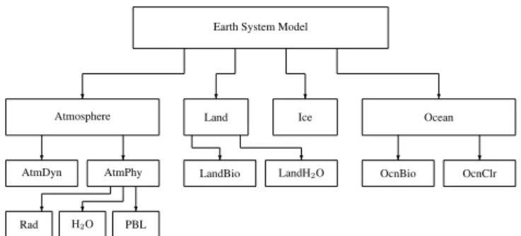
Earth System Model
? ? ? ?
Atmosphere Land Ice Ocean
? ? AtmDyn AtmPhy ? ? ? Rad H2O PBL ? ? OcnBio OcnClr ? ? LandBio LandH2O
Figure 1. Notional architecture of an ESM: The model is composed of components (or sub-models) each of which is itself composed of components representing a group of one or more related processes. For example, within the atmosphere, the dynamical core (AtmDyn) is only one component, alongside the “physics” (AtmPhy), which itself has subcomponents for radiation (RAD), clouds and moisture (H2O),
planetary boundary layer (PBL), and so on. The list shown here is clearly not exhaustive, and one could easily imagine further recursive trees within any component shown.
The computational characteristics of ESM components can be quite diverse: a land component for instance may have no data dependencies across cells, but highly multivariate representations of ecosystem dynamics inside a cell; whereas an atmospheric dynamical core (dycore) may only encompass a few key variables representing momentum, mass and energy, but have strong cross-cell dependencies, which inhibit scaling. This is one reason why it is hard to define kernels, or “mini-apps”, representative of an ESM. Even for a single component, such as a dycore (which solves the equations of fluid flow for atmosphere or
5
ocean), there is remarkable diversity of methods and approaches across models. Spectral, finite-difference (FD), finite-volume (FV), and finite-element (FE) methods are all in use in the world’s major ESMs, as are both structured and unstructured grid approaches.
The dycore is quite often taken to be representative of the ESM as a whole. Dycores, regardless of numerics and mesh choice, generally exhibit weak scaling, i.e., the concurrency achieved scales with the problem size2. Scaling is capped beyond
10
some point for a fixed problem size, beyond which strong scaling is difficult to achieve. Thus, one may run a problem at higher resolution in the same time consuming more resources on a given machine (which might include a higher cost incurred in increased time resolution as well), but a model at fixed resolution is capped in terms of time to solution, absent advances in 2Since concurrency is usually achieved with a mixture of thread-based (shared-memory, such as OpenMP) and processor-based (distributed-memory, such
as MPI) parallelism, we prefer to use the neutral term concurrency here, to indicate the number of concurrent executing elements, regardless of how this is achieved.
5
Figure 1. Notional architecture of an ESM: the model is composed of components (or sub-models), each of which is itself composed of components representing a group of one or more related processes. For example, within the atmosphere, the dynamical core (AtmDyn) is only one component, alongside the “physics” (AtmPhy), which itself has subcomponents for radiation (RAD), clouds and moisture (H2O), planetary boundary layer (PBL), and so on. The list shown here is clearly not exhaustive, and one could easily imagine further recursive trees within any component shown.
unit (GPU) and many-integrated core (MIC) technology has pushed the percent of peak down into the single digits, as re-vealed by the HPCG / HPC ratio (see http://goo.gl/yy6ZJ4)1. This trend warrants curbing one’s enthusiasm when looking at peak-flop ratings of today’s most powerful machines. 2.2 Computational performance of ESMs
Earth system models have always presented a particular set of issues for performance on HPC architectures. To begin with, there is the problem of complexity. Climate science has been described as an attempt to simulate “the time evo-lution of the Earth system, a complex evolving mixture of fluids and chemicals in a very thin layer atop a wobbling, spinning sphere with an unstable surface and a molten in-terior, zooming through space in a field of extra-terrestrial photons at all wavelengths. Between sea and sky [lies] that thin layer of green scuzz that contain[s] all the known life in the universe, which itself [is] capable of affecting the state of the whole system” (Balaji, 2013). This growth in sophisti-cation implies that the construction of an ESM (Fig. 1) now involves large development teams, consisting of specialists in different aspects of the climate system such as atmospheric and oceanic dynamics, atmospheric chemistry, biosphere and land hydrology, and so on, with the whole system held to-gether by a software framework. The framework may pro-vide infrastructure services such as parallelism and I/O, as well as a superstructure, expressing the algorithms of cou-pling between components.
The computational characteristics of ESM components can be quite diverse: a land component for instance may have no data dependencies across cells but highly multivariate
rep-1“Architectural Surprises Underpin New HPC Benchmark
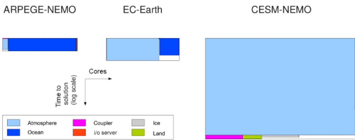
Figure 2. Component layout of three ESMs, in processor-time space (time increasing downward). Each box represents a component which is integrated either concurrently (coarse-grained concurrency; see text), in which case it is shown alongside the other components running at the same time, or sequentially, in which case it is shown below the previous component. The bounding rectangle shows the total cost of the coupled system, including waiting times due to load imbalance. Adapted from Fladrich and Maisonnave (2014).
resentations of ecosystem dynamics inside a cell, whereas an atmospheric dynamical core (dycore) may only encompass a few key variables representing momentum, mass, and en-ergy but have strong cross-cell dependencies, which inhibit scaling. This is one reason why it is hard to define kernels, or “mini-apps”, representative of an ESM. Even for a single component, such as a dycore (which solves the equations of fluid flow for atmosphere or ocean), there is remarkable di-versity of methods and approaches across models. Spectral, finite-difference (FD), finite-volume (FV), and finite-element (FE) methods are all in use in the world’s major ESMs, as are both structured and unstructured grid approaches.
The dycore is quite often taken to be representative of the ESM as a whole. Dycores, regardless of numerics and mesh choice, generally exhibit weak scaling; i.e., the concurrency achieved scales with the problem size2. Scaling is capped
beyond some point for a fixed problem size, beyond which strong scaling is difficult to achieve. Thus, one may run a problem at higher resolution in the same time, consuming more resources on a given machine (which might include a higher cost incurred in increased time resolution as well), but a model at fixed resolution is capped in terms of time to solution, absent advances in hardware or algorithm. Some-times, adding more local physics (which does not involve distributed data dependencies) can improve scaling (the abil-ity to use more computing capacabil-ity), but even that does not improve time to solution. We next address this issue of com-plexity of models as we go from dycores to full ESMs.
While dycores often consume the bulk of the resources de-voted to performance engineering, their performance charac-teristics are not in fact representative of a whole ESM. This
2Since concurrency is usually achieved with a mixture of
thread-based (shared-memory, such as OpenMP) and processor-thread-based (distributed-memory, such as MPI) parallelism, we prefer to use the neutral term concurrency here, to indicate the number of concurrent executing elements, regardless of how this is achieved.
is because of the complexity inherent in climate modeling. Beyond the dycore, there are many other components. As shown in Fig. 1, these may comprise the “physics”, which is then further composed of components representing radia-tive transfer, clouds and convection, the planetary boundary layer (PBL), and so on. Many physical variables, of O(100) in modern ESMs, are needed to represent the full physics. Of-ten these are local processes, which may not be a problem for scaling but which significantly alter the load per thread. Sec-ondly, the number of variables (each typically a 3-D array) is a significant burden on memory. The scaling behavior can be significantly different when “fully loaded” with physics.
A second feature of multi-component codes is that an ESM is quite often set up to run multiple component codes con-currently as separate executables each with their own pro-cessor decomposition. This component architecture of ESMs is quite diverse (Alexander and Easterbrook, 2015), but typi-cally most include at least two such components set up to run concurrently, in a mode we term coarse-grained concurrency (Balaji et al., 2016). This raises issues of load balance, con-figuring components to execute in roughly the same amount of time, so no processors sit idle. In such a “coupled” set-ting, components may not be able to run at their individual optimal scaling point, but rather at the scaling point which is optimal for the ESM as a whole. In addition, there are over-heads associated with the coupling software itself. Compo-nents are generally allowed to have their own grid resolu-tions and timescales, and the coupler is responsible for ex-changing information in a manner respecting numerical sta-bility, accuracy, and, above all, conservation of the quantities exchanged among the components. The coupling overhead must be taken into account in an ESM performance study. Coarse-grained concurrency may be increasingly prevalent in ESM architectures in the future, because of current hardware trends (Balaji et al., 2016). The parallel component layout of some typical ESMs is shown in Fig. 2.
Some components are scheduled to run concurrently, but usually are not exactly load-balanced, leaving load imbal-ance as blank spaces on the processor-time diagram, as shown. Other components may run serially at the end of other components. We will revisit this aspect of coupling below in Sect. 3.3.
A third consequence of complexity is that a large num-ber of variables needs to be analyzed in scientific experi-ments involving ESMs. I/O is often ignored in scaling stud-ies (including the standard HPC benchmarks other than those specifically measuring I/O performance), although rigorous and careful studies, such as the recent AVEC report (http:// www.nws.noaa.gov/ost/nggps/dycoretesting.html), do take it into account. Both synchronous (blocking) and asynchronous (non-blocking) I/O subsystems are in use in ESMs. In the first instance, they will directly contribute to the measured time to solution, and in the latter, they will contribute to the cost in terms of additional processors devoted to I/O. In terms of real performance, it is important to include I/O, as the rel-ative cost of computation and I/O is essential to defining a balanced machine suitable for ESMs.
We come to the third axis (see Sect. 1) along which Earth system modeling consumes computing power, that of ensem-ble size. The underlying dynamics of an ESM are chaotic, with a sensitive dependence on initial conditions, as has been known since the pioneering studies of Lorenz (1963). In climate and weather modeling, chaotic uncertainty is cap-tured by running an ensemble of simulations with slightly perturbed initial conditions and examining the results in the form of a probability distribution rather than as an exact out-come. This has serious implications for understanding the performance of ESMs, as now the science is limited by the capacity of the computer (i.e., aggregated simulation time across an ensemble) rather than by its capability (simulation time of a single instance). ESMs for science may be run in both capability mode (fastest time to solution for a single in-stance) or capacity mode (best use of a computer allocation for an ensemble of runs), depending on need; both need to be assessed.
A final point regarding Earth system modeling is that runs may be resident on a system for very long times. Climate simulations often run for centuries or millennia of simulated time, taking wallclock time measured in months. This means that in actual practice, the time to solution is dependent on many factors, including the stability of the machine, the de-sign of the queuing system, and the robustness of the work-flow.
In summary, Earth system modeling has a particular com-putational and data profile which must be taken into account in measuring the computational “performance” of a given model on a given machine. The profile of climate computing is that of a multi-scale, multi-physics code, organized into a hierarchy of components that may be scheduled serially or concurrently, held together by sophisticated coupling algo-rithms that themselves carry a cost. Individual components
generally exhibit weak scaling, are memory-bound, and may carry a significant I/O load. The models are executed for very long periods of time, so that a significant cost is associated with the workflow and machine policies enabling sustained sequences of jobs. Finally, the models are sometimes run at their optimal speed, but quite often require large ensembles of simulations, so that they are in practice optimized for ca-pacity rather than capability.
2.3 Real model performance: an alternative approach The premise of this paper is that existing measures of com-putational performance do not give the Earth system science community adequate information about the actual model performance obtained in running scientific production runs. Such information is needed for a range of practical applica-tions which go beyond the prediction of performance for tra-ditional applications such as benchmarking new machines, to include the decisions needed to plan scientific experiments with real codes on specific hardware.
These features, required to assess real model performance in a scientific domain, require understanding of the particu-lar domain computational profile – in this case, the profile summarized at the end of Sect. 2.2 – and development of ap-propriate metrics to study performance.
Typical questions that ESM users have when they plan or run an experiment include the following.
– How long will the experiment take (including data transfer and post-processing)?
– How many nodes3 can be efficiently used in different
phases of the experiment?
– Are there bottlenecks in the experiment workflow, either from software or from system policies, such as queue structure and resource allocation?
– How much short-term/medium-term/long-term storage (disk, tape, etc.) is needed?
– Can/should the experiment be split up into parallel chunks (e.g., how many ensemble members should be run in parallel)? What is the best use of my (limited) allocation?
Although these questions are clearly related to the com-putational performance of ESMs, they are not answered by examination of flops or speed-up curves.
We therefore propose an alternative approach. We have devised a set of computational performance metrics that di-rectly address the concerns of this domain of science. The metrics have been chosen to satisfy several conditions:
3Although the number of computational elements is measured in
cores, allocation is usually done in units of nodes of, say, 32 cores sharing memory.
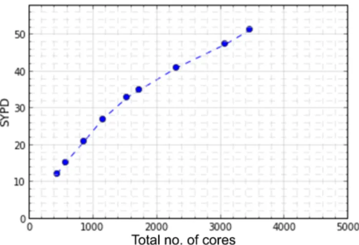
Figure 3. Scaling behaviour of a GFDL model. It illustrates that the model could be run at 50 SYPD in capability, or speed mode, but in practice is most often run at the shoulder of the curve, at around 35 SYPD, which gives the best throughput.
– they are universally available from current ESMs, and applicable to any underlying numerics, as well as any underlying hardware architecture;
– they are representative of the actual performance of the ESMs running as they would in a science setting, not under ideal conditions, or collected from representative subsets of code;
– they measure performance across the entire lifecycle of modeling, and cover both data and computational load; and
– they are extremely easy to collect, requiring no special-ized instrumentation or software, but can be acquired in the course of routine production computing.
These metrics will form the basis of a framework for rou-tinely collecting these data from large coordinated modeling experiments. They are intended to serve as an adjunct to tra-ditional, more idealized, measures of performance. They will allow the community as a whole to have a unified basis to evaluate technological advances through the lens of commu-nity concerns and to articulate commucommu-nity needs for compu-tational and data architecture.
3 The CPMIP metrics
We propose below in Sect. 5 a systematic effort to col-lect metrics for a variety of climate models participating in common experiments. This proposed model intercomparison project (MIP) is to be called CPMIP: the computational per-formance MIP. The metrics proposed take into account the structure of ESMs and how they are run in production. Issues addressed include the following.
1. Models can have two optimal points of interest: one for speed (minimizing time to solution, maximizing simu-lated years per day or SYPD), the second for best use of a resource allocation (minimizing compute hours per simulated year, or CHSY). A single ESM experiment may contain both phases. For instance, a climate exper-iment is often initialized from an idealized initial state, and a long “spinup” phase (measured in centuries for an AOGCM, millennia if the model includes a carbon cy-cle for instance; see, e.g., Dunne et al., 2012) where we would run the model in speed or capability mode (the two terms are used interchangeably). After the spinup phase we have a near-equilibrium initial state of the cli-mate which may be used to seed many experiments in parallel, in which case we would switch the configura-tion to throughput or capacity mode. We call these the S-mode and T-mode, respectively.
Figure 3 illustrates the S- and T-modes from a typical scaling study, in this case from a GFDL model configu-ration called c96l32 running on a platform called c3. We see that the model is capable of running at 50 SYPD (simulated years per day, a quantity precisely defined below in Sect. 3.2). However, by then, the scaling is be-ginning to suffer. In practice, we find that the best use of a computer allocation is to run the model at 35 SYPD, where the performance slope starts to change, indicat-ing loss of scalindicat-ing. The best throughput, measured in CHSY (also defined below in Sect. 3.2), is achieved at the lower processor count (1200 instead of 1600). 2. Computational cost scales with the number of degrees
of freedom in the model. We factorize this number sepa-rately into resolution (number of spatial degrees of free-dom) and complexity (number of prognostic variables). This separation is useful because performance varies inversely across resolution and complexity in weak-scaling models.
3. ESMs generally are configured to run more than one component concurrently: we need to measure load bal-ance and coupler cost.
4. A vast number of variables is often used in the code, which is likely to aggravate the memory-boundness of models. While the theoretical minimum of one word (usually double-precision, or 8-byte) per variable per spatial degree of freedom is unavoidable, it is useful to measure memory bloat and excess copies of data made by the code, the compiler, or libraries. We do not neces-sarily consider the word bloat to be pejorative: some of the extra copies might be needed for scientific reasons, such as halos (local caches of portions of neighboring domains in distributed memory), or to provide registers for accumulating time means of time-step data. But, rea-sons notwithstanding, these extra copies of data do in-deed increase the memory requirements. And some data
copies remain mostly outside user control (e.g., system I/O buffers).
5. Models configured for scientific analysis bear a signifi-cant I/O load, which can interfere with optimization of computational kernels. I/O may be synchronous (block-ing) or asynchronous (non-block(block-ing). Typical and max-imum simulation data intensities (GB/CH) are useful measures for designing system architecture.
6. A full production climate model run, which may last weeks or months of investigator time, may be subject to delays not having to do with actual computational per-formance. We need a measure of these machine policy or workflow-related issues, a metric which indicates the need to devote resources to system (including manage-ment and queuing policies) and workflow issues rather than optimizing code.
To cover this list of concerns, we propose the following list of metrics, and indicate how this may be measured. (Recall that one prime consideration in the choice of metrics is the ease of collection.)
3.1 The CPMIP metrics: model and platform
We begin with metrics describing the model and the plat-form. The model is described by two basic characteristics. Resolution is measured as the number of grid points (or
more generally, spatial degrees of freedom) NX×NY× NZ per component, denoted by Gc (where the
sub-script denotes a model component with an independent discretization). The resolution of the ESM is simply G ≡P cGc. Gc ≡ NH × NZ, (1) G ≡ X c Gc, (2)
where NH and NZ are the spatial degrees of freedom in the horizontal and vertical dimensions, respectively. Given the small vertical extent of the atmosphere and ocean relative to the horizontal extent in any ESM, it is customary to represent them separately. NZ is thus the number of model levels; NH represents the hori-zontal degrees of freedom, which for instance may be NX × NY in a conventional FD or FV discretization, or the number of spherical harmonic elements retained un-der truncation in a spectral model, or the number of hor-izontal elements in an unstructured FE code.
We also additionally require a representative (noting that non-uniform grids are the norm) horizontal and ver-tical cell size for broad comparison purposes, 1xcand
1zc, reported in kilometers. The resolution is static in-formation about the model and part of its configuration.
Complexity is measured as the number of prognostic vari-ables per component, Vc. This is also static, but if
not available directly from the model configuration or code, it can be computed by dividing the size Scof the
restart file (containing the complete state) per compo-nent, measured in words (e.g., 8 bytes for double pre-cision) divided by Gc. The complexity of the model is
C ≡P
c Vc. The total degrees of freedom in the model is
F ≡P cGcVc. Vc ≡ Sc/Gc/8 (3) V ≡ X c Vc (4)
Note that the method of computing it from the restart file size assumes that only one copy of the model state is saved (i.e., no intermediate restarts). It further assumes that only one time level of any variable is saved in the restart file. For models that use multiple level time-stepping schemes, there could be several time levels saved in the restart file. For proper restarting of a model with leapfrog time-stepping, for instance, both the cur-rent and prior states of a variable need to be saved. Thus, using the restart file method to estimate complexity is to be used with caution: it is better to have more di-rect methods of computing Vc, the number of prognostic
variables.
Other methods for evaluating complexity (e.g., Méndez et al., 2014) are more based on evaluations of the model code itself, e.g., counting lines of source code. Our ex-perience is that models of equal complexity in terms of the range of physical, chemical, and biological process represented, vary considerably in terms of code, which appears to us not to provide a useful measure of com-plexity. We further note that most models are coded with a plethora of options, most of which are not exercised in any one model instance, thus resulting in a lot of “dead code”.
The platform is a description of the computational hard-ware.
Platform There is a wide variety of machine descriptors, which can be confusing. With the computing hierar-chies in place, terms like processor, processing element or PE, and even computing core, become hard to com-pare across machines. However, the term core still has some universality as a concept, as a machine is often characterized by its core count, though what constitutes a core may not be strictly comparable across disparate hardware. With that concept, the two additional mea-sures universally understood are the clock speed (usu-ally reported in inverse time, so that larger is faster) in GHz, and the theoretically possible number of double-precision operations per clock cycle – which we term
clock-cycle concurrency. All three measures can be ob-tained across the span of today’s architectures, includ-ing GPUs, MICs, BlueGene, and conventional proces-sors.
Note that there are additional numbers of interest, such as memory and file-system characteristics. These are highly configuration-specific and quite often het-erogeneous. We propose two additional descriptors: chip name (e.g., Knights Landing) and machine name (e.g., titan). These should allow one to find links to configuration-specific information about the platform. 3.2 The CPMIP metrics: computational cost
SYPD are simulated years per day for the ESM in a 24 h pe-riod on a given platform. This should be collected by timing a segment of a production run (usually at least a month, often 1 or more years), not from short test runs. This is because short runs can give excessive weight to startup and shutdown costs, and distort the results fol-lowing Amdahl’s law. This is measured separately in throughput and speed mode.
ASYPD is the actual SYPD obtained from a typical long-running simulation with the model. This number may be lower than SYPD because of system interruptions, queue wait time, or issues with the model workflow. This is measured for a long production run by measur-ing the time between first submission and the date of arrival of the last history file on the storage file system. This is measured separately in throughput and speed mode. For a run of N years in length,
ASYPD ≡ N tN−t0
, (5)
where t0is the time of submission of the first job in the
experiment, and tN is the time stamp of the history file
for year N.
CHSY are core hours per simulated year. This is measured as the product of the model runtime for 1 SY and the number of cores allocated.4This is measured separately
in throughput and speed mode.
Parallelization is measured as the total number of cores NP allocated for the run. Note that NP = CHSY × SYPD/24.
JPSY is the energy cost of a simulation, measured in Joules per simulated year. Energy is one of the key drivers of computing architecture design in the current era.
4There may be some “rounding up” involved, as allocations are
usually done on a node basis, and all cores on a node are charged against the allocation, regardless of whether or not they are used.
While direct instrumentation of energy consumption on a chip is still something in development, we generally have access to the energy cost associated with a plat-form (including cooling, disks, and so on), measured in kWh (= 3.6×10⁶Joules) over a month or a year. Given the energy E in Joules consumed over a budgeting in-terval T (generally 1 month or 1 year, in units of hours), and the aggregate compute hours A on a system (total cores ×T ) over the same interval T , we can measure the cost associated with 1 year of a simulation as follows:
JPSY ≡ CHSY × E/A. (6)
Note that this is a very broad measure, and simply pro-portional to CHSY on a given machine. But it still is a basis of comparison across machines (as E will vary). In future years as on-chip energy metering ma-tures and is standardized, we can imagine adding an “actual Joules per SY (AJPSY)” measure, which takes into account the actual energy used by the model and its workflow across the simulation lifecycle, including computation, data movement, and storage. These mea-sures are similar in spirit to some prior meamea-sures of “en-ergy to solution” (Bekas and Curioni, 2010; Cumming et al., 2014; Charles et al., 2015). The FTTSE metric of Bekas and Curioni (2010) is very similar to the AJPSY metric proposed here, and which we believe will replace JPSY in due course, when direct metering becomes rou-tinely available.
3.3 The CPMIP metrics: coupling, memory and I/O Coupling cost measures the overhead caused by coupling.
This can include the cost of the coupling algorithm it-self (which may involve grid interpolation and compu-tation of transfer coefficients for conservative coupling) as well as load imbalance, when concurrent components finish at different rates, potentially leaving some PEs idle. It is possible to measure the two separately, but it involves somewhat subtle instrumentation, and may not be measurable in a uniform way across the range of ESM architectures used in the community (Alexander and Easterbrook, 2015). This is because load imbalance can manifest itself as time spent in the coupler (which is actually being spent in a spin-wait loop). We instead just choose to measure it as the normalized difference be-tween the time-processor integral for the whole model vs. the sum of individual concurrent components, or
C ≡
TMPM−P
cTcPc
TMPM , (7)
where TMand PMare the runtime and parallelization for
components. Graphically, it can be seen as the “white area” for any ESM layout diagram like that of Fig. 2. It involves a minimum of instrumentation to measure time spent on each component. These involve inserting simple timing calipers such as MPI_WTime() around components, excluding wait. While this may be consid-ered extra “instrumentation”, these are universally avail-able basic routines, and indeed it would be a wonder if any ESM interested in performance did not have these embedded already.
Memory bloat is the ratio B of the actual memory size to the ideal memory size Mi, defined below. The measured
runtime memory usage M on the system (often called “resident set size”, or RSS) is divided between instruc-tions and data, of which we are interested mainly in the latter. The RSS high-water mark is often published in the job epilog, failing which we supply a small code (26 lines of C; see Sect. 6), which can be called at the end of a model run and which will report the RSS high-water mark on any Linux-derived operating system. The por-tion of memory devoted to instrucpor-tions is measured by taking the size of the executable files X produced during compilation, of which one copy is stored on every pro-cessor. This may be an overestimate on systems where instructions are paged in, or shared between applica-tions, so the correction for instruction size is to be ap-plied with care. The ideal memory size is the size of the complete model state, which in theory is all you need to hold in memory, the rest being in principle computable from the state variables. Thus,
Mi ≡ X c Sc, (8) B ≡ M −NP × X Mi . (9)
Note that the “ideal” memory size is truly a utopian measure, and we never expect to get close in prac-tice. Rather, it serves as a normalization factor allow-ing us to compare across different model characteristics (Sect. 3.1) and platforms. As we shall see, the value of Bis found to be O(10 − 100).
Unusually large numbers relative to other configura-tions can alert us to excessive buffering and other is-sues. Also, we generally aspire to have memory scaling codes, where memory usage remains roughly constant across PE counts. It will generally not stay exactly con-stant because of the presence of halos. For instance, for a logically rectangular grid with a halo size of 2 in X and Y , and a 20 × 20 domain under decomposition, the 2-D array area including halos is 576 instead of 400, for a bloat factor of 1.44. The same model decomposed to a 10 × 10 domain will have an array area of 196 instead of 100, increasing the bloat to 1.96. This number might
be somewhat larger for algorithms that use “wide ha-los” (Balaji, 2001). However, these factors are still small compared to the bloat caused by global arrays, which will cause memory to grow on a curve quadratic with the PE count (assuming 2-D domain decomposition). Avoiding the use of global arrays is generally consid-ered a useful approach in an era where memory move-ment is considerably more expensive than arithmetic. Data output cost is the cost of performing I/O, and is the
difference in cost between model runs with and with-out I/O. This is measured as the ratio of CHSY with and without I/O. This is measured differently for sys-tems with synchronous and asynchronous I/O. For syn-chronous I/O where the computational PEs also perform I/O, it requires a separate “No I/O” run where we mea-sure the fractional difference in cost:
D ≡CHSY − CHSYno I/O
CHSY . (10)
For models using asynchronous I/O such as XIOS, a separate bank of PEs is allotted for I/O. In this case, it may be possible to measure it by simply looking at the allocation fraction of the I/O server, without needing a second “no I/O” run.
D ≡PM−PI/O
PM (11)
However, there may be additional computations per-formed solely for diagnostic purposes; thus, the method of Eq. 10 is likely more accurate. Note also that if the machine allocates by node, we need to account for the number of nodes, not PEs, allocated for I/O.
Data intensity is the measure of data produced per compute hour, in GB/CH. This is measured as the quotient of data produced per SY, easily obtained from examining the output directories, divided by CHSY.
4 Results from several ESMs
We present a spectrum of results from several ESMs to il-lustrate the power of the CPMIP approach. These are to be considered preliminary or suggestive findings.
Some of the metrics we collect are properties of the model which do not change however the model is run, but some are properties of the exact experiment for which it is used. In par-ticular, the I/O properties (data output cost and data intensity) will depend on the diagnostics required by the experiment.
Similarly, ASYPD is simulation dependent, depending not only on the model configuration, but also on the background
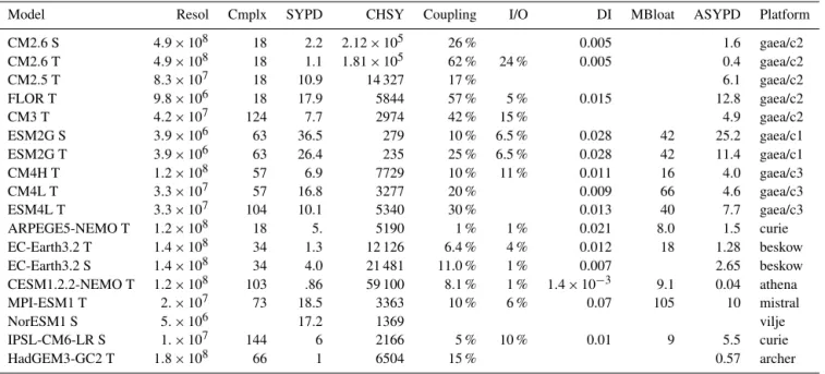
Table 1. Results from several ESMs. Not all the cells are currently filled, but we propose to collect these systematically in the full-scale CPMIP project. See the text for an explanation and a discussion of the terms.
Model Resol Cmplx SYPD CHSY Coupling I/O DI MBloat ASYPD Platform
CM2.6 S 4.9 × 10⁸ 18 2.2 2.12 × 10⁵ 26 % 0.005 1.6 gaea/c2 CM2.6 T 4.9 × 10⁸ 18 1.1 1.81 × 10⁵ 62 % 24 % 0.005 0.4 gaea/c2 CM2.5 T 8.3 × 10⁷ 18 10.9 14 327 17 % 6.1 gaea/c2 FLOR T 9.8 × 10⁶ 18 17.9 5844 57 % 5 % 0.015 12.8 gaea/c2 CM3 T 4.2 × 10⁷ 124 7.7 2974 42 % 15 % 4.9 gaea/c2 ESM2G S 3.9 × 10⁶ 63 36.5 279 10 % 6.5 % 0.028 42 25.2 gaea/c1 ESM2G T 3.9 × 10⁶ 63 26.4 235 25 % 6.5 % 0.028 42 11.4 gaea/c1 CM4H T 1.2 × 10⁸ 57 6.9 7729 10 % 11 % 0.011 16 4.0 gaea/c3 CM4L T 3.3 × 10⁷ 57 16.8 3277 20 % 0.009 66 4.6 gaea/c3 ESM4L T 3.3 × 10⁷ 104 10.1 5340 30 % 0.013 40 7.7 gaea/c3 ARPEGE5-NEMO T 1.2 × 10⁸ 18 5. 5190 1 % 1 % 0.021 8.0 1.5 curie EC-Earth3.2 T 1.4 × 10⁸ 34 1.3 12 126 6.4 % 4 % 0.012 18 1.28 beskow EC-Earth3.2 S 1.4 × 10⁸ 34 4.0 21 481 11.0 % 1 % 0.007 2.65 beskow CESM1.2.2-NEMO T 1.2 × 10⁸ 103 .86 59 100 8.1 % 1 % 1.4 × 10⁻³ 9.1 0.04 athena MPI-ESM1 T 2. × 107 73 18.5 3363 10 % 6 % 0.07 105 10 mistral NorESM1 S 5. × 106 17.2 1369 vilje IPSL-CM6-LR S 1. × 107 144 6 2166 5 % 10 % 0.01 9 5.5 curie HadGEM3-GC2 T 1.8 × 10⁸ 66 1 6504 15 % 0.57 archer
workload on the machine, which is the reason why we require this to be obtained from a long model run (so the background differences are averaged out).
For model intercomparison, the best understanding of model differences will be obtained when the differing mod-els are being used for the same experiment. Hence, the full power of the method will only be apparent when we have systematically collected these metrics in conjunction with a major multi-center modeling project. A plan to do so in as-sociation with CMIP6 is outlined below in Sect. 5.
4.1 Speed and throughput modes
Performance results from HPC codes are often presented in the form of scaling curves, with time to solution plotted at various processor counts. A typical inference from such a plot is to identify models that scale well, i.e., close to an ideal scaling curve that points to the “strong scaling” limit. Recall that under strong scaling, the time to solution decreases in-versely with the number of processors, i.e., half the time to solution for twice the assigned processing.
Most models scale less than perfectly, so in general sci-entific projects make compromises. There are two poten-tial optima: one is to optimize time to solution by apply-ing the maximum resource possible (the point at which the scaling curve saturates, so that adding more PEs does not improve time to solution); or alternately, pick a spot lower down the scaling curve for the maximum aggregate simu-lated years for an ensemble of model runs within a given al-location. In terms of the metrics defined in Sect. 3, we refer to these modes as the speed (S) or capability mode which maximizes SYPD, and the throughput (T) or capacity mode,
which minimizes CHSY. Table 1 gives examples of GFDL high-resolution model CM2.6 (Griffies et al., 2015), for in-stance, which can be run at 2 SYPD, but in practice is most often run at 1 SYPD, which is the CHSY optimum. An ESM example is also shown (ESM2G, Dunne et al., 2012), where the 26 SYPD T configuration is usually run, but during model spinup (which is a single instance running, not an ensem-ble) the S configuration is used. ESM spinup often requires O(1000) years (Dunne et al., 2013), where raw speed is of the essence: we see that even at 40 SYPD a time on the order of months is needed simply to generate an equilibrated initial condition for a set of experiments.
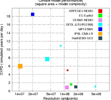
4.2 Complexity, resolution, and performance
We assume in the rest of the discussion that the runs being analyzed are in T-mode, as they would be run in production. In this section we show a comparison across several ESMs. The comparisons here necessarily have considerable scatter as they represent codes with differing levels of performance, and different hardware as well. Nonetheless, the inverse re-lationship between resolution and time to solution is seen in the scatter plot of Fig. 4. Complexity, a second major deter-minant of performance, is shown as the size of the square on the scatter plot. Broadly, on similar performing hardware, we expect to see one group of models of limited complexity in one cluster on the resolution–SYPD slope, and another simi-lar cluster for high-complexity models. Models lying consid-erably below the cluster representing their complexity class may indicate a need for performance improvement, either in the code or in hardware. In general, we can identify the low-complexity models as AOGCMs, and the high-low-complexity
Figure 4. Performance, resolution, and complexity for a subset of ESMs from Table 1, in throughput mode.
models as ESMs, which add chemistry and carbon to the mix. These results will of course be significantly clearer when we have a substantial database of results, allowing us to subse-lect based on platform, for example.
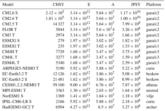
4.3 Energy consumption
We present here the JPSY metric for select models, with the caveats mentioned above in Sect. 3.2, namely that the energy costs are based on representative machine averages.
Table 2 shows the energy costs of the various model sim-ulations in Table 1. The current results show that they are drawn from platforms with rather similar energetic profiles, and most of the variance in energetic costs comes from vari-ations in CHSY. Below in Sect. 4.7 we show a comparison of the same model on different platforms, with a substantial difference in energy profile. This will be seen to have signif-icance in machine evaluation.
4.4 Coupler overhead and load imbalance
One area of concern in coupled modeling is the cost of the coupling itself. There are two aspects to this.
– When components are running concurrently there are synchronization costs which arise when the components must exchange data; i.e., a component that finishes early must wait for its boundary condition received from an-other component. Also, components may have restric-tions on the layout (i.e., the PE count can only be dis-cretely altered). Second, the load is often a function of the actual narrative of events taking place in the model (e.g., convective activity). Thus it may not be possible
to maintain an exact load match between components. This is usually done by trial and error and left fixed for the duration of an experiment.
– A second cost is that of the coupler itself: this includes the cost of conservative interpolation between indepen-dent model grids, as well as any other computations per-formed during the transfer. This can include computing fluxes, transforming quantities (for instance, different components may have differing units or sign conven-tions for certain variables). In some cases transfer co-efficients are computed on an intermediate “exchange grid” (e.g., Balaji et al., 2006).
These are both unavoidable costs of coupling; therefore, as outlined in Sect. 3, we have chosen to measure them as one: the coupling cost is the processor-time integral of the difference between the total cost of the coupled system and the integrated cost of individual components, depicted graph-ically as the white area outside any component in Fig. 2.
One area of concern is whether the coupler costs rise with resolution. A comparison of two models built from the same modeling system (the low-resolution ESM2G vs. high-resolution CM2.6) in Table 1 shows that the coupler cost, cluding load imbalance, increases from 1 to 25 % with the in-crease in resolution. This comparison is made in the S-mode. At lower PE counts (T-mode) it is more difficult to estab-lish load balance because of layout restrictions as described above. Here the cost comparison across low and high reso-lutions rises from 25 to 62 %. Further examination indicates that this is an example of a model configuration that was in-sufficiently tuned for performance before starting a produc-tion run, and indeed a much better load balance could have been achieved. This inference is given a boost when we com-pare CM4H and CM4L, which are differentiated by high and low ocean resolution. Here in fact the coupling cost is lower in the high-resolution configuration. We therefore conclude that there is no evidence of a loss in coupling performance with resolution, and the anomalous result for CM2.6 is prob-ably due to an imperfect configuration. We present this as evidence that systematic collection of the CPMIP metrics would help identify such cases during setup for production, rather than post facto, as in this table.
4.5 I/O issues
As noted in Sect. 3, I/O load is measured here by comparing a production run with no diagnostic output against a regular production run. We see a generally modest cost ranging from 6.5 % for low-resolution models up to 24 % at high resolu-tion. (The CM2.6 run shown here contains an eddy-resolving ocean, and the high cost of I/O in that run is associated with high-frequency output for analyzing eddy statistics: Griffies et al., 2015).
In other modeling systems with asynchronous I/O (such as the XIOS system developed in France; see
Table 2. Energy cost per simulated year (Joules) in several of the configurations listed in Table 1. See Sect. 4.3 for an explanation of the terms. Energy and aggregate core hours are reported for 1 month.
Model CHSY E A JPSY Platform
CM2.6 S 2.12 × 10⁵ 3.14 × 10¹² 5.64 × 10⁷ 1.17 × 10¹⁰ gaea/c2 CM2.6 T 1.81 × 10⁵ 3.14 × 10¹² 5.64 × 10⁷ 1.00 × 10¹⁰ gaea/c2 CM2.5 T 14 327 3.14 × 10¹² 5.64 × 10⁷ 7.99 × 10⁸ gaea/c2 FLOR T 5844 3.14 × 10¹² 5.6 × 1074 3.26 × 10⁸ gaea/c2 CM3 T 2974 3.14 × 10¹² 5.64 × 10⁷ 1.66 × 10⁸ gaea/c2 ESM2G S 279 1.97 × 10¹² 3.02 × 10⁷ 1.82 × 10⁷ gaea/c1 ESM2G T 235 1.97 × 10¹² 3.02 × 10⁷ 1.53 × 10⁷ gaea/c1 CM4H T 7729 1.68 × 10¹² 3.47 × 10⁷ 3.75 × 10⁸ gaea/c3 CM4L T 3277 1.68 × 10¹² 3.47 × 10⁷ 1.59 × 10⁸ gaea/c3 ESM4L T 5340 1.68 × 10¹² 3.47 × 10⁷ 2.59 × 10⁸ gaea/c3 ARPEGE5-NEMO T 5190 5.92 × 10¹² 5.88 × 10⁷ 5.22 × 10⁸ curie EC-Earth3.2 T 12 126 1.62 × 10¹² 3.86 × 10⁷ 5.08 × 10⁸ beskow EC-Earth3.2 S 21 481 1.62 × 10¹² 3.86 × 10⁷ 8.99 × 10⁸ beskow CESM1.2.2-NEMO T 59 100 9.00 × 10¹² 6.76 × 10⁷ 7.87 × 10⁹ athena MPI-ESM1 T 3363 1.30 × 10¹² 2.65 × 10⁷ 1.64 × 10⁸ mistral NorESM1 S 1369 1.41 × 10¹² 1.64 × 10⁷ 1.18 × 10⁸ vilje IPSL-CM6-LR S 2166 5.92 × 10¹² 5.88 × 10⁷ 2.18 × 10⁸ curie HadGEM3-GC2 T 6504 4.27 × 10¹² 8.5 × 10⁷ 3.27 × 10⁸ archer
http://forge.ipsl.jussieu.fr/ioserver and Joussaume et al., 2012), the same cost is measured by seeing how many PEs are assigned to I/O relative to the rest of the model.
Another useful metric here is the data intensity defined in Sect. 3. It shows the rate of data production per hour of pro-cessing, in units of GB/CH. We see the data intensity de-creasing as resolution increases, but staying proportional to increases in complexity.
4.6 Workflow costs
We see examples in Table 1 where there is a substantial discrepancy between ASYPD and SYPD; for instance, the ESM2G T-mode only achieves 11 SYPD in practice against an expected 26 SYPD. This indicates a need for closer exam-ination. There could be several reasons for this.
– The workflow system could be introducing inefficien-cies. This would be identified by a detailed examination of the run logs, or whether the delays are induced during data transfer or post-processing, for instance.
– the queuing system could be introducing delays. Sched-uler logs would identify whether there is excessive queue wait time, in which users may seek to change the queuing policies at their compute site, or else find a “sweet spot” for the T-mode that best aligns with those policies.
– The run might have been interrupted by the scientist for various reasons; for example, they might choose to “pause” the run to perform some preliminary analysis.
In this case, we indeed discovered that there were sig-nificant gaps between output file timestamps at several points in the run, indicating that these were deliberate pauses.
These results indicate the utility of the CPMIP metrics for diagnosing problems associated with model workflow, which have as much impact on realized performance as algorithms and computational hardware.
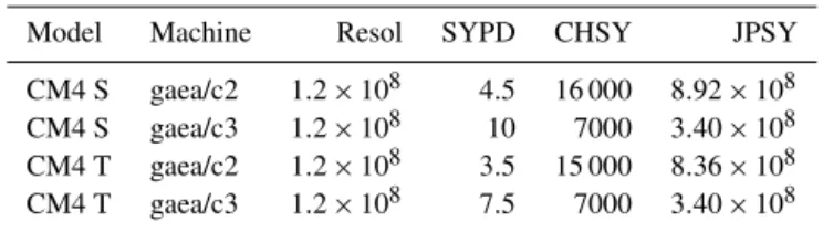
4.7 Hardware comparison
One of the most impactful uses of the CPMIP metrics is in getting comparisons of actual performance improvements from new hardware. As we have emphasized in this paper, nominal measures of performance provided by vendors such as clock speed in GHz, or maximum theoretical flops, do not provide clear indications of what actual increase in perfor-mance will be realized in practice on the actual applications run on the machine. In Table 3, we provide a direct com-parison of the same codes on the current machine and on a new acquisition. NOAA has recently upgraded the tech-nology on its flagship climate computer Gaea. The results of Table 1 were acquired on Gaea’s c1 and c2 partitions in 2014, when it was a Cray XE6 (120 320 AMD Interlagos cores rated at 3.6 GHz on a Cray Gemini fabric). In early 2016, a c3 partition was added, a Cray XC40 consisting of 48 128 Intel Haswell cores rated at 2.3 GHz but with higher clock-cycle concurrency, and the next-generation Aries inter-connect fabric (see Table 4). Given the higher rated
proces-Table 3. Results comparing the same model in both speed (S) and throughput (T) mode on different hardware.
Model Machine Resol SYPD CHSY JPSY
CM4 S gaea/c2 1.2 × 10⁸ 4.5 16 000 8.92 × 10⁸
CM4 S gaea/c3 1.2 × 10⁸ 10 7000 3.40 × 10⁸
CM4 T gaea/c2 1.2 × 10⁸ 3.5 15 000 8.36 × 10⁸
CM4 T gaea/c3 1.2 × 10⁸ 7.5 7000 3.40 × 10⁸
sors and smaller number of cores, what is the true compari-son across these machines?
Table 3 provides some answers. The CM4 model currently in development at GFDL shows a modest increase in cost as we increase the PE count, beginning to saturate in perfor-mance as we get to 4.5 SYPD (indicated by the increase in CHSY between rows 1 and 3). Over the same range, we are able to demonstrate an increase on the new hardware c3 from 7.5 to 10 SYPD, at no increase in CHSY. We can infer three things.
– Core for core, the new machine shows a speedup of 2.2X, which one could not have inferred from the clock ratings. However, the total number of cores has dropped by 2.5X. Thus, in aggregate, c3 provides about 87 % (2.2 / 2.5) of the capacity of the older c1 and c2 par-titions combined, for the GFDL workload. Note, how-ever, that the PF rating of c3 (the product of columns 3, 4, and 5 in Table 4) is considerably higher than c1 and c2 combined (1.77 PF vs. 1.12 PF). This shows the pitfalls of using petaflop ratings to infer the aggregate performance of a machine.
– A second inference is that the next-generation network (Cray Aries over Gemini) is showing a manifest in-crease in performance, with the same CHSY in both configurations (i.e., with different numbers of PEs), whereas there was a drop in performance on the older hardware. Additional data on very high-resolution mod-els, not shown here, show that the scaling increase re-sults in vastly increased performance at very high PE counts, pushing the per-core performance difference to nearly 3X.
– A third and equally intriguing result is apparent from the energy analysis in the JPSY column. We see substantial decreases in the energy cost of simulation, with JPSY dropping by 60 % in migrating from c2 to c3, partly due to the lower CHSY, but also partly attributable to energy efficiency of the hardware. This translates into a very concrete and substantial fall in the total cost of simulation science over the lifetime of the machine. Comparisons of this nature based on CPMIP metrics can yield extremely useful material for comparing hardware and
for interpreting benchmark results. A broad database of re-sults across models and machines will also allow centers to gain useful insights about their own workload from acquisi-tions at other centers.
In future, modeling centers are likely to be distributing work across heterogeneous systems: this information could additionally aid in matching model configurations (e.g., res-olution and complexity) to hardware.
The platforms used in this study are listed in Table 4. 5 Summary and future work
Computational performance is one of the most important constraints in the design of Earth system modeling experi-ments. These constraints force compromises between resolu-tion, complexity, and ensemble size, all of which have serious scientific implications. This paper proposes several metrics for assessing real computational performance of ESMs, and as an aid in experimental design and strategic planning, in-cluding future computer acquisitions consistent with a mod-eling center’s mission.
It is our contention that traditional measures of computa-tional performance do not provide the necessary input for ex-perimental design and planning. The kinds of questions sci-entists face include the following.
– For a given experimental design, what can I afford to run?
– If I add complexity (such as adding a biogeochemistry component to an AOGCM), what will I have to sacrifice in resolution?
– How much computing capacity do I need to participate in a campaign like CMIP6 (Meehl et al., 2014)? How much data capacity?
– Do the queuing policies on the machine hinder the sus-tained run of a long-running model?
– During the spinup phase, how long (in wallclock time) before I have an equilibrium state?
The metrics we propose are designed to address questions such as these, not easily answered from flops and scaling curves. They are specifically designed to be universal (i.e., not based on a specific component hierarchy), very easy to collect (no specialized software or instrumentation), and re-flective of actual performance in production.
As the energy cost of computing (Cumming et al., 2014; Charles et al., 2015) is increasingly becoming the limiting factor in large-scale computing, we expect that our machine-average measure of model energy consumption JPSY will need to be replaced by a more accurate measure of energy consumption AJPSY, using fine-grained hardware energy
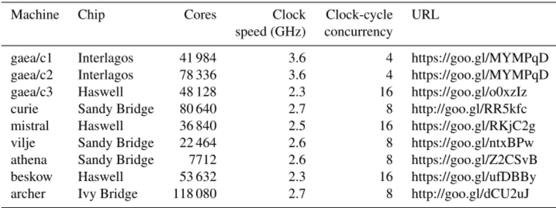
Table 4. Details of platforms used in this study. The product of cores, clock speed, and clock-cycle concurrency should yield theoretical peak speed, but as we see in the results of, and discussion around, Tables 1 and 3, the actual performance is rather different.
Machine Chip Cores Clock Clock-cycle URL
speed (GHz) concurrency
gaea/c1 Interlagos 41 984 3.6 4 https://goo.gl/MYMPqD
gaea/c2 Interlagos 78 336 3.6 4 https://goo.gl/MYMPqD
gaea/c3 Haswell 48 128 2.3 16 https://goo.gl/o0xzIz
curie Sandy Bridge 80 640 2.7 8 http://goo.gl/RR5kfc
mistral Haswell 36 840 2.5 16 https://goo.gl/RKjC2g
vilje Sandy Bridge 22 464 2.6 8 https://goo.gl/ntxBPw
athena Sandy Bridge 7712 2.6 8 https://goo.gl/Z2CSvB
beskow Haswell 53 632 2.3 16 https://goo.gl/ufDBBy
archer Ivy Bridge 118 080 2.7 8 http://goo.gl/dCU2uJ
metering. In doing so, we will need to track energy consump-tion across the entire modeling lifecycle, including computa-tion, data movement, and storage. Regardless of how energy per simulation unit is measured, we believe these metrics will play a substantial role in selecting technologies, as we will be able to demonstrate direct benefits in operating costs per “unit of science”, such as a simulated year. Technolo-gies that appear weaker in “core-for-core” comparisons may show up as stronger in energy comparisons. Across machines and models, we can imagine debates about certain choices of hardware being “slower but greener”, or algorithms that are “less accurate but more eco-friendly”. We believe these con-siderations will enrich the landscape of design of both hard-ware and simulation softhard-ware and workflow.
Other questions may be asked as well, which are more project-specific. For instance, the CMIP experimental pro-tocol is fundamentally dependent on an extensive process of data standardization, using tools such as the Climate Model Output Rewriter (CMOR, http://www2-pcmdi.llnl. gov/cmor). While the standardization is a tremendous boon to data consumers, the data producers often chafe at the somewhat onerous process of standardization. We could imagine project-specific metrics such as measuring the time spent making the CMIP runs, the total computational load of CMIP, and the time spent in post-model data standardiza-tion. The set of metrics may thus evolve in the future, with project-specific addenda.
We propose a systematic campaign to collect the basic metric set in this paper routinely for CMIP6 before consid-ering its growth and evolution. This will be done using cur-rently planned systems of model documentation such as ES-DOC (http://es-doc.org) (Lawrence et al., 2012). This com-parative study of computational performance across models and machines, a CPMIP, will be an invaluable resource to the climate modeling community. Each center will individually be able to identify inefficiencies in their modeling lifecycle and seek to address them. The comparative data will allow one center to predict the performance it will achieve on a ma-chine available at another center. We propose to build such
an emulator tool backed by the CPMIP database for this pur-pose. It will allow centers to define the optimal compute–data balance on future acquisitions. Finally, it will allow the Earth system modeling community as a whole to identify machine configurations and policies most apt to the kinds of science we hope to undertake in the future.
6 Data and code availability
The code for computing memory usage within the model (see Sect. 3.3) is provided in memuse.c (https://github.com/ NOAA-GFDL/FMS/blob/master/memutils/memuse.c). It is to be run on each PE and will provide the resident set size for that PE on any Linux-based operating system.
All the data used in the tables and figures of this study are available in raw form in a public Dropbox folder (see https://goo.gl/Fxl5XX). As stated in the paper, the ESDOC project will be collecting and publishing the data systemati-cally during CMIP6 from all participating models.
Acknowledgements. V. Balaji is supported by the Coopera-tive Institute for Climate Science, Princeton University, award NA08OAR4320752, from the National Oceanic and Atmospheric Administration, US Department of Commerce. The statements, findings, conclusions, and recommendations are those of the authors and do not necessarily reflect the views of Princeton University, the National Oceanic and Atmospheric Administration, or the US De-partment of Commerce. He is grateful to the Institut Pierre et Simon Laplace (LABEX-LIPSL) for support in 2015, during which drafts of this paper were written.
The research leading to these results has received funding from the European Union Seventh Framework program under the IS-ENES2 project (grant agreement no. 312979).
B. N. Lawrence acknowledges additional support from the UK Natural Environment Research Council.
We thank Lucas Harris and Ron Stouffer of NOAA/GFDL, as well as Claire Levy of IPSL and an anonymous reviewer, for insightful and thorough reviews of this article, down to the last comma.