Crustal structure from teleseismic bodywave data

(1)

Crustal Structure from Teleseismic Bodywave Data

by

John Edward Foley

M.S., Boston College (1984)

B.S., University of Lowell (1981)

Submitted to the Department of Earth, Atmospheric, and Planetary

Sciences

in partial fulfillment of the requirements for the degree of

Doctor of Science

at the

MASSACHUSETTS INSTITUTE OF TECHNOLOGY

June 1990

@

Massachusetts Institute of Technology 1990

All rights reserved

Signature of A uthor ...

.... . ....

... .. .. ....

...

Department c Earth, At

heric, Qd Planetary Sciences

SMay

25, 1990

Certified by.

(

Accepted by...

..

9 M. Nafi Toksiz

Professor of Geophysics

Thesis Advisor

Thomas H. Jordan

Chairman

Department of Earth, Atmosphgc,

JU c -H f

WaiII Ns

V UIV 'r!,bgl

and Planetary Sciences

(2)

**'*~--Crustal Structure from Teleseismic Bodywave Data**

by

John Edward Foley

Submitted to the Department of Earth, Atmospheric, and Planetary Sciences on May 25, 1990, in partial fulfillment of the

requirements for the degree of Doctor of Science

Abstract

In this thesis we have developed and implemented a series of techniques to determine infor-mation about the crustal velocity structure of the earth beneath a network of seismic stations from the analysis of teleseismic P-waveforms. We examined the usefulness of methods which utilize vertical component teleseismic P-seismograms recorded on 2 seismic monitoring net-works. The first is located in the northeastern United States and is utilized as a test area for the new methods, and the second is in Larderello, Italy, the site of one of the world's largest geothermal energy production facilities which is currently being explored with a variety of geological and geophysical methods.

The main general conclusion of this study is that the analysis of vertical component tele-seismic P-waveforms can provide very useful information about the crustal velocity structure of the earth. It has long been recognized that the delays in travel time of direct P-waves can image the broad lateral velocity variations in the earth. We have demonstrated that the application of a tomographic method based on these observations can provide a good estimation of the lateral extent of the low velocity zone in Larderello. To improve this model of the earth structure we examined the waveforms for primary reflections from deep velocity discontinuities which either have regional extent or are isolated to the vicinity of in-dividual receivers. The measure of the travel times from these phases (although much more difficult to make than the direct arrival) hold valuable information about the crust. We developed two methods to extract this information from the vertical component teleseismic P-waveforms. The first is the application of a simulated annealing technique to the problem of relative travel time determination and works on the premise that within a window in each waveform a wavelet is common to all stations recording the same event. We use this opti-mization method to locate the Moho in New England and to determine accurate measures of direct arrivals in the Larderello data. The second method relies upon an important data transformation which simplifies and regularizes the waveforms. This transformation is a two-step process, where we first determine the source wavelet common to all receivers for each recorded event and then convert each source into a simple and repeatable zero-phase wavelet. Once transformed, we take advantage of the wide variety of event incidence angles present in the New England and Larderello data sets. Each primary reflection two-way travel time is dependent on the event incidence angle (or ray parameter), and we exploit this dependency

(3)

to determine the relative travel times and average velocities to major discontinuities in the crust by using a ray parameter trajectory stacking scheme (called the rpt method).

To extract all of the available information about the crustal velocity structure out of teleseismic waveforms, one must incorporate the entire waveform into the analysis. To this end, we have developed and applied a waveform inversion method to refine the details of the velocity model sketched by the previous techniques. This method is based on the calculation of sensitivity functions, or partial derivatives, of the predicted seismogram to changes in each of the parameters which are used in the calculation of the synthetic waveform. This waveform matching scheme uses the misfit to the data and the Frechet kernel to update the model, and with this process we can resolve important velocity features in the crust.

In addition to these general conclusions we have determined a number of specific impor-tant and interesting details about the velocity structure of the Larderello geothermal area. The travel time residual inversion yielded information about the size and extent of the low velocity feature in the crust. This intrusive body is about 20 km by 20 km in lateral extent and exists from depths of about 6 km to below 40 km. The strong travel time residual in the area (about 1 second over about 30 km) indicates a region of intense reduced velocity to by at least 20% (melts of igneous rocks are a reduced in velocity by 30 to 40%). The

rpt method was applied to the Larderello data to help clarify this picture of the crust, and

we found that beneath most stations in the region, strong velocity discontinuities exist at depths of 20 to 25 km. This regional feature is interrupted in the central portion of the area where a negative gravity anomaly is strongest and where temperatures are most elevated. This area has a number of more isolated velocity contrasts.

Our waveform inversion technique confirms many of the findings of the previous applica-tions to teleseismic data and supplements them with detailed information about the crustal velocity structure (particularly in the upper 3 to 10 km). This part of the crust is diffi-cult to image with conventional reflection techniques but holds important information about the tectonic evolution of the region as well as information pertinent to geothermal explo-ration. We were able to demonstrate with this preliminary study of the velocity structure in Larderello that analysis techniques utilizing vertical component teleseismic waveform data (direct arrivals, primary reflections and full P-waveforms) and two data enhancement tech-niques (simulated annealing and source equalization) can reveal some of the fine details of the velocity structure of the crust.

Thesis Advisor: M. Nafi Toks6z Title: Professor of Geophysics

(4)

Acknowledgments

I would like to thank a few people who provided help, insight and support to me while I was a student at MIT. First and foremost I would like to thank Nafi Toksiz, my thesis advisor and director of the Earth Resource Laboratory, for his help in putting my effort in its proper scientific perspective. With his wide range of experiences and overview of the the geophysical sciences and geophysical community he has been able to teach me a great deal about many important aspects of becoming an effective and productive scientist. I was also quite fortunate to to have had the advice, encouragement and support of John Ebel from Boston College. John is a consummate seismologist and has educated me immeasurably over the years.

While at MIT I was a member of the Earth Resources Laboratory. Being associated with this group has truly rounded my education and prepared me to leave MIT with numerous tangible skills beyond those related to earthquake seismology. Nafi, Roger Turpening and Arthur Cheng have kept this unique and productive environment alive and have provided an excellent facility in which to work. They deserve many thanks. The lab is run by an excellent staff and I thank Sara Brydges, Jane Maloof, Al Taylor, Naida Buckingham, Liz Henderson and Sue Turbak for all their help.

In the Italian part of my research effort I was lucky to have had the help of Fausto Batini of ENEL. His assistance, along with that of the talented group in his Larderello lab, made the geothermal project a pleasure to work on.

The friends I've made while at MIT have made the last 5 years at ERL a very positive experience. In particular I would like to thank Ed Reiter, Bob Cicerone, Chuck Doll, Jim Mendelson, Fatih Guler, Jane Maloof and Delaine Thompson for their constant good nature, proper perspective and friendship.

Most of all I would like to express my thanks to my wife Judy who never let me take myself too seriously.

(5)

Chapter 1 INTRODUCTION

Thesis Objectives

The amplitudes and travel times of seismic body waves are strongly affected by the media through which they travel and can be measured and analyzed to determine the properties of the earth. This study is undertaken in an effort to derive information about the earth's ve-locity structure from the analysis of teleseismic P-waveforms. There are two main objectives in this research, both of which focus on the crustal velocity structure near seismic recording stations. The first of our goals is to develop and then apply teleseismic waveform and travel time methods to the specific problem of velocity structure characterization of the Larderello Geothermal Field (Figure 1), an area in central Italy. This important geothermal region has been the focus of numerous geophysical and geological studies undertaken in order to develop a more clear understanding of the crustal structure and crustal dynamics of this area. The tectonic setting of this region has a complicated modern expression, and a clear and accurate account of the tectonic evolution of this area is essential to interpret other geophysical and geological observations. With this study, we add a new set of well controlled observations based on the analysis of teleseismic waveforms to the base of information which presently exists for Larderello, and we develop a model from these velocity structure observations which helps to clarify some of the issues that remain for a better tectonic understanding of the Larderello Geothermal Area.

(9)

seismic velocity analysis techniques aimed at imaging the velocity structure of the crust utilizing vertical component teleseismic P-waveforms recorded on seismic networks. This type of data is quite abundant from numerous seismic networks operating around the world which are generally deployed to monitor local and regional seismic activity. In this re-search we limit the development and application of waveform analysis techniques to vertical component seismograms in order to maintain the widest possible base of application of the techniques. Generally, vertical P-waveforms have been used primarily in travel time residual studies based on the relative arrival time of the direct P-wave. The timing and amplitudes of phases arriving after the direct P-wave which originate from the structure near the receiver and are recorded on vertical component sensors have not been used to refine crustal velocity structures. We evaluate the potential of this under-utilized set of observations by applying various vertical waveform analyses to seismograms collected on the Larderello Seismic Net-work and to the seismograms recorded in New England on the North East United States Seismic Network. We test our analysis methods on waveforms recorded in New England since the velocity structure in this area is simpler than in Larderello and is known fron other seismic studies.

Teleseimic Waveform Data

The focus of this thesis is on vertical component teleseismic P-waveform data collected on seismic monitoring networks. Teleseismic P-waves travel from the earthquake source region through the body of the earth and arrive at the recording network generally at steep incidence angles (Figure 2). Because of large epicentral distances, the curvature of the wavefront is small when it arrives at the recording array and can be represented by a plane (Aki and Richards, 1980). This assumption greatly simplies all of the following analyses.

The data used in this research comes from two seismic monitoring networks which were established to monitor local and regional seismic activity. The first is located in Larderello, Italy in southwest Tuscany and is operated by the Ente Nazionale per l'Energia Elettrica (referred to as ENEL), a national energy agency in Italy. It is comprised of 26 stations (Figure 3). The area covered by the network is about 30 by 40 km in extent and the average station spacing is about 6 km. We use 101 teleseismic events recorded during the period

(10)

1986-1988 recorded on the Larderello Seismic Network in this study.

The second seismic network is located in the northeastern United States and is referred to as the NEUSSN. This network is operated principally by four separate monitoring groups: Earth Resources Laboratory at the Massachusetts Institute of Technology, Weston Observa-tory of Boston College, Lamont Doherty Geological ObservaObserva-tory of Columbia University, and the Earth Physics Branch of Canada. The NEUSSN is comprised of about 100 stations over an area roughly 400 km by 200 km in extent (Figure 4) and has a variable station spacing averaging about 40 km. We have collected 148 teleseismic events recorded on the NEUSSN

during the period 1985 - 1987 from earthquakes with magnitudes ranging from MB 4.8 to

Ms 7.3. Both of the networks used in this study record teleseismic waveforms with short

period, vertical component sensors at most of their stations.

Some Advantages of Teleseismic Data

Traditionally, there have been two conventional ways to examine the crust with seismic waves. The first is with reflection techniques, where energy is put into the earth at the surface and reflected waves, originating from interfaces below, are recorded on the surface at near vertical angles. The second approach is to use refracted waves, where sources on the surface generate waves which are recorded at various distances from the source. Both of these methods are important and have numerous useful applications. However, when the deep crust and upper mantle are being investigated, they both have serious limitations. With reflection methods energy transmission to great depths is problematic, and with refraction methods lateral spatial resolution is generally limited. The use of teleseismic P-wave data, (direct P-wave arrivals, later reverberations from the crustal discontinuities, or the the entire P-waveforms) to determine crustal features avoids some of the limiting complications of both refraction and reflection approaches. Since teleseismic P-waves travel short lateral distances in the crust (on the order of 10 km), regional scale travel path averaging does not occur. This is in contrast to refraction studies where shot-to-receive distance of over 100 km are required to image the lower crust (Jarchow and Thompson, 1989). The use of teleseismic data helps us discriminate between local irregular velocity structures near individual stations and regional trends of the crustal velocity structure. The second advantage comes from the

(11)

frequency band of teleseismic waveforms recorded on the NEUSSN and ENEL networks, which is generally in the range of 0.5-3.0 Hz. Teleseismic data has a lower frequency content than typical reflection sources (10 to 50 Hz) and refraction experiments (2-15 Hz). Resolution of fine velocity structures is reduced with teleseismic waveform methods due to the lower frequencies in the data. However, less attenuation occurs at these frequencies and more energy returns to the surface from deep reflectors. Seismic waves in the frequency band used here are more reflective than higher frequency sources used in reflection seismic methods from laminated layers which have been proposed to exist at the base of the crust (Hale and

Thompson, 1982).

In order to take advantage of these attributes of teleseismic waveform data, special analy-sis and signal-to-noise ratio enhancement techniques are needed to overcome some limitations of teleseismic P-wave data recorded on typical seismic networks. For the direct P-wave ar-rival recorded at teleseismic distances from a typical earthquake with a magnitude of 6.0, the signal-to-noise ratio is generally great enough to allow for accurate measurements of the travel time of the direct arrival. However, later arriving phases originating as reflections from crustal discontinuities beneath a station typically have amplitudes between 0.05 and 0.2 of the direct arrival and have signal-to-noise ratios which are very low (typically at or below 1.0). In addition to the ambient environmental noise we observe a high degree of incoher-ent scattered energy on most teleseismic waveforms which are due to lateral heterogeneities in the crust (Dainty, 1990). These arrivals produce a scattered coda wave after the direct arrival and often have greater amplitudes than the arrivals from large scale velocity discon-tinuities in the crust. Without the amplification of the coherent part of the seismograms we are restricted to analysis of the direct arrivals exclusively for determining crustal velocity features. The second major difficulty with teleseismic P-wave data is the lack of knowledge of the source function incident at the base of the crust. The waveforms recorded at a station on a seismic network are affected by the earthquake source, the raypath through the body of the earth, and local crustal effects. If we want to isolate the crustal response beneath a recording site, we must remove the effects in the waveform which come from other sources.

(12)

described in Chapter 2, is based on the idea of simulated annealing optimization (Rothman, 1986) and helps to determine travel times in noisy data. The second method, called source equalization, helps us to determine and remove the source and propagation effects in our data. The source equalization method is divided into two parts; the first part is used to determine the source wavelets which are common to all seismograms recorded on a network from a single event, and the second part removes these effects with a modified deconvolution

process. This method is described in Chapter 4.

Crustal Structure Applications

In this thesis we apply five different methods to the problem of crustal velocity structure characterization which utilize vertical component teleseismic P-waveforms. These include:

1. Relative travel time residual inversions of the direct P-wave arrivals,

2. Mapping of coherent reflectors beneath New England with the application of a simu-lated annealing optimization procedure,

3. Scanning source equalized data recorded at individual stations for incident angle de-pendent reflections,

4. Forward modeling source equalized and stacked waveform data and 5. Inverse modeling source equalized and stacked waveform data.

1.2 The Larderello Geothermal Region

The Larderello Geothermal Field is located within the complex structure of the Apennines Mountains which run down the center of the Italian Peninsula (Figure 1). Most Italian geothermal settings lie in the inner Apennines (toward the Tyrrhenian Sea) and are char-acterized by a complicated tectonic history. Larderello is in southwestern Tuscany and has had a tectonic history similar to that of other geothermal areas which exist in the NW-SE trending tectonic belt (Mt Amiata, Mt. Cimino, Mt. Vesuvious, Mt Etna, for example). Figure 5 (taken from Batini et al., 1983) shows a schematic diagram of the geologic setting of the Larderello Geothermal Field. This area is characterized by 3 main geologic units. From the top down we see a cap rock made up of a sequence of clayey flysch and conglomerates

(13)

deposited during the post-Alpine transgressive phase which is underlain by a series of folded and thrusted sedimentary nappes. This complex of tectonic wedges was overthrusted during the Alpine orogeny and is made up of limestones and anhydrites. Beneath this sedimentary pile is a metamorphic basement composed of phyllites and quartzites strongly corrugated during the Hercynian orogeny. The upper sedimentary rocks of this area area have been ex-tensively studied in an effort to understand the processes controlling geothermal production (Batini and Nicolich, 1984). Within the basement metamorphic rocks a dominant seismic marker was discovered which is believed to represent the top of contact aureole associated with Late Apline magmatic intrusive activity (Batini and Nicolich, 1984). This feature (re-ferred to as the K horizon) marks a petrophysical change in the rocks and is thought to be a zone of highly fractured rocks filled with steam or hot fluids. A more complete description of the geologic and tectonic background of the Tuscan region as well as a description of other geophysical observation made in Larderllo can be found in Chapter 7 and a detailed discussion is available from Puxeddu (1984) and Boccaletti et al. (1985).

1.3 Introduction to the New England Application

The application of teleseismic waveform analysis techniques to data collected in New England is undertaken in an effort to test the procedures developed in this study and to assess to usefulness of the techniques in typical local earthquake monitoring settings.

This intraplate region was built by a long progression of intense mountain building episodes. The general northeast trend in the geologic features (Merrimack Synclinorium, Bronson Hill Anticlinorium, Gaspe Synclinorium, etc., Figure 6) is due to the large scale compressive forces associated with repeated opening and closing of the proto--Atlantic Ocean

(Taylor and Toksoz, 1979; Williams and Hatcher, 1982). The contacts between major

provinces are believed to represent individual continental collision sutures (Rast and Ske-han, 1983), and from the complicated nature of the surface geology and tectonic history of the NEUSSN, one might expect the deep crustal structure to vary widely across the re-gion. Refraction and reflection results do indicate that the crust in New England is quite heterogeneous. An extensive and well controlled refraction experiment was undertaken in

(14)

central Maine in 1984 and a detailed map of Moho topography resulted from this experiment (Luetgert et al., 1987). This region is utilized as a control area in our simulated annealing analysis. This is the only large scale refraction experiment conducted in the New England until 1988, and results from this more recent project are not yet available. A large number of smaller, more passive, and therefore less well controlled refraction experiments have been conducted in the region (Leet, 1941; Linehan, 1962; Katz, 1955; Dainty et al., 1966; Chiburis et al., 1977; Schneck et al., 1976; Mitronovis, 1985). The models of the deep crustal velocity structure vary widely among these studies.

Reflection techniques deployed in the New England area have had difficulty in quantifying deep crustal velocity characteristics (Ando et al., 1984; Brown et al. 1983, Oliver et al., 1983; Mereu et al., 1986; Phinney, 1986; Hutchinson, 1986; and Stewart et al., 1986). Ando et al. (1984) were able to image to depths of only about 15 km in the Adirondacks, for example. The reflectivity of the New England Moho discontinuity can be quite variable. Mereu et al. (1986), for example, observe sharp Moho reflections in the Central Gneiss Belt of southern Quebec but very weak reflections only 100 km to the southwest in the Ottawa Graben.

1.4 Roadmap and Description of Methods

We are interested in studying the structure and tectonic evolution in Larderello and have developed and implemented a number of varied but related methods to help characterize the velocity structure beneath the seismic network operating in that area. We also test these methods on data collected on the NEUSSN to assess the usefulness of these techniques in a more typical seismic monitoring setting. Since the goals of this research are different in the NEUSSN and ENEL applications, each method is applied differently in the two areas, with emphasis always placed on the Larderello case where more dense spatial coverage has the overwhelming advantage of inherently better resolution. The relatively close station spacing in Larderello (about 6 km) as opposed to the spacing in New England (about 40 km) greatly amplifies the applicability of all of the teleseismic techniques.

We describe in the paragraphs below and show in Table 1-1 the outline of this study. In each chapter we present a general introduction to the current topic, the goals of the

(15)

appli-cation and the data requirements. We then discuss the theoretical justifiappli-cation of each of the approaches, as well as the key implementation issues whenever applicable. We generally present only a brief discussion of the results from the Larderello applications in the individ-ual method chapters and leave the interpretation and discussions for the last chapter where all of the results are combined.

Simulated Annealing for Teleseismic Phase Selections

In Chapter 2 we look at the problem of teleseismic phase arrival time determination using the simulated annealing optimization approach. With this method we search the waveforms collected on the NEUSSN for Moho reflections arriving in the coda of the direct arrival. In the ENEL application we use this technique to accurately determine relative direct P-wave arrival times. The simulated annealing method recasts the phase identification problem as an optimization problem where we essentially test all possible combinations of network ar-rival configurations for each event by probabilistically updating the configuration state of the current model.

Travel Time Residual Inversion

In conjunction with the simulated annealing method of Chapter 2, we use the travel time residual observations of 101 teleseismic events recorded on Larderello network to determine the broad nature of the low velocity anomaly which exists in the center of the area. This study is presented in Chapter 3, and the results are fully interpreted in Chapter 7 where all the results from Larderello are gathered. The approach we have taken comes from the well studied Aki et al. (1977) methodology which has been applied in numerous volcanic areas around the world (see Iyer 1988, for a review).

Source Equalization

In Chapter 4 we present a method by which we can overcome many of the limitations associ-ated with vertical component teleseismic P-waveforms. This is accomplished by removing all common source and common propagation effects from each individual trace and re-shaping

(16)

each natural source wavelet into a simple and repeatable source pulse. This transformation facilitates cross-event stacking and makes available a number of useful procedures to examine later arrivals in the seismograms.

Ray Parameter Trajectory Stacks

In Chapter 5 we introduce a new method to determine crustal velocity characteristics be-neath a single recording station. This technique is called the ray parameter trajectory stacking method (or rpt method), and with it we utilize the wide range of event incidence angles (and therefore ray parameters) which arrive at each station. With this technique we scan source equalized waveforms recorded at a single station for coherent arrivals by sys-tematically testing all possible crustal velocity discontinuity configuration states. With this method we are able to determine the two-way travel time to all major reflectors beneath a station and can make estimates of interval velocities from deep layers.

Waveform Modeling

Like the rpt modeling of Chapter 5, Chapter 6 utilizes the major simplifications brought about by the source equalization method of Chapter 4. In this final methods chapter we re-cast the time-domain forward waveform matching process as a maximum likelihood inver-sion procedure. We discuss the development of the teleseismic waveform inverse problem, as well as model parameterization and implementation issues.

Conclusions

The last chapter of this thesis deals with the combination and interpretation of results of the various methods. We pull together all the new information we have determined about the Larderello geothermal area and combine the results with the wide base of information already known about the region. This information is then integrated to produce a model for this dynamical geothermal region. Lastly, we assess the usefulness of teleseismic data to determine crustal velocity structure and present recommendations for future application of the techniques developed in in this study.

(17)

TABLE 1: Roadmap of Thesis

Chapter Description of Application Data Used Application Area

2 Simulated annealing optimization Deep Crust Synthetic Tests and

method for travel time selections Arrivals New England Moho

3 Simulated annealing optimization Direct P- ENEL; Direct P-Wave

Arrivals Trav Time Residuals

4 Source Equalization; effective Entire Synthetic Tests

source calculations, and Waveforms New England Data

generic wavelet transformations ENEL Data

5 Ray Parameter Trajectory Stacks Post-Source Test Data

To Primary NEUSSN (11 Stations)

Arrivals ENEL (Entire Network)

6 Waveform Modeling Entire NEUSSN (2 Stations)

(18)

A Li

IPI3NeOTIHEMA A GEOTHIUmAL oISIENSIVE AXEA4

Figure 1: The Larderello geothermal field is located about 100 km south of Florence, Italy and lies within the complex structure of the Apennines which run down the center of the Italian Peninsula. Most Italian geothermal settings lie in the inner Apennines (toward the Tyrrhenian Sea) and are characterized by a complicated tectonic history.

(19)

-eismic Monitoring Network

Moho Discontinuity

Figure 2: The focus of this thesis is on vertical component teleseismic P-waveform data collected on seismic monitoring networks. Teleseismic P-waves travel from the earthquake source region through the body of the earth and arrive at the recording network generally at steep incidence angles. Because of large epicentral distances, the curvature of the wavefront is small and can be represented by a plane.

(20)

43.3 - 1U I

SASS SDALSCAPRADI

' MINI SCAP RA I

MLUC

PADU VALE FROS 'TRAV

MN43.1

LAGDSV CORN SINI

STTA FRAS CRpE LURI

43.1 CRDP

PLUZ MBAM

431.6 10.7 10.B 10.9 11.0 11.1 11

LONCITUDE

Figure 3: The seismic network at Larderello is operated by the Ente Nazionale per l'Energia Elettrica (ENEL), a national energy agency in Italy, and it has 26 uniform calibrated stations.

(21)

JKM MIM HKM BPM TRM NMA 0 0 1 MIT

Earth Physics Branch Lamont Doherty Weston Observatory

Figure 4: Northeastern United States Seismic Network has about 100 seismic stations and is operated by four separate monitoring groups; Earth Resources Laboratory at the Mas-sachusetts Institute of Technology, Weston Observatory of Boston College, Lamont Do-herty Geological Observatory of Cloumbia University and the Earth Physics Branch of Canada.

(22)

- SW- -NE-SASSO 22 RIBATTOLA T 00-0 -m -1500 -1500- -22-0--260 -2500- -35000-000LEGEN 4 000-NEOGENIC SEDIMENTS . Miocene (U Cretaceous) CANETOLO COIPLEX (Paleocene-U. Eocene

(U. Oliocene-L. Miocene)

(U. Cretaceous-1igocene) CALCARE SELCIFERO FOR ATION

_ CALCARE MASSICCI FORMATION SEVAI:ITIC AND DOLWITIC SERIES

(u. rri ) AND TECTONIC SLICES COMPLEX

SVERRTANOL FOMTION

(M.-U. Trias)

rN-TI GROUP

LLADI INFERItaeous R GROP M. Paeozoc to

Precambri an

- MICASCHIST _ GNEISS

K SEISMIC REFLECTING HORIZON

Figure 5: Schematic cross-section of the Larderello Geothermal Field (taken from Batini et

al., 1983) is characterized by 3 main units (from top down); a sequence of clayey flysch and conglomerates which is underlain by a series of folded sedimentary nappes. These are in turn underlain by a basement of metasediments. The K Horizon is a key petrophysical marker believed to represent the top of an extensive contact aureole.

(23)

00

Figure 6: The northeastern United States is an intraplate region built by a long progression of intense mountain building episodes. The general NE trend in the geologic features

(Merrimack Synclinorium, Bronson Hill Anticlinorium, Gaspe Synclinorium, etc., Figure 6) is due to the large scale compressive forces associated with repeated opening and closing of the proto-Atlantic Ocean and the contacts between major provinces are believed to represent individual continental collisions sutures. This simplified tectonic map of New

England is taken from Taylor and Toksoz (1979).

? I

EXPLANATION

& Thrust fault, barbs on upper block m-u Normal foaut, hochures on downthrown sie

STRATIFIED ROCKS

: Cenezoic glacial deposits

Triassic red beds SCorboniferous

SSilurian - Devonian eugeoclinal rocks

Cambrian -Ordovician foreland rocks

]

Cambrian - Ordovician deformed miogeoclinal rocks

0 Cambrian - Ordovician ougeoclinal rocks

[ Precambrian rocks of the eastern block

Precambrian uplifts, Grenville basement

Precambrian Grenville basement

IGNEOUS ROCKS

[]

Mesozoic White Mountain Plutonic Series

SDevonian

New Hampshire Plutanic Series Cambrian -Ordovician serpentinites, ultramofics

(24)

Chapter 2 SIMULATED ANNEALING WITH

TELESEISMIC DATA

2.1 Introduction

We explained in Chapter 1 that one of the basic problems in analyzing earth structure using teleseismic observations is the inherently low signal-to-noise ratio observed on many seismograms. This feature of teleseismic data makes the accurate determination of travel times subject to some uncertainty depending on the impulsiveness, frequency content and amplitude of the arriving signal. In this chapter we present a method which overcomes this liability of teleseismic data through the application of an optimization scheme based on the simulated annealing concept. There are many useful and practical applications which can be employed to determine the nature of the velocity structure of the crust from teleseismic data if we can determine accurate measures of the relative travel times of various teleseismic phases arriving at 'Stations in a seismic network. We develop the method of automated, simulated annealing based phase identification in this chapter and apply this technique to the problem of determining the depth to the Moho in the New England area. In the following chapter we show that the delay times of direct teleseismic P-wave arrivals (derived with the simulated annealing method) can be used to determine important broad features of the velocity structure of the crust and upper mantle beneath the Larderello Seismic Network.

(25)

The process of isolating and accurately measuring the arrival time of a particular phase on a vertical component teleseismic P-waveform is subject to inherent uncertainties (Iyer, 1975; Foley and Toksoz, 1987; VanDecar and Crosson, 1990, for example). The source of the difficulty in reading travel times in teleseismic data exists for the following reasons:

1. The signal-to-noise ratio of the direct arrival or a reflected arrival from a velocity discontinuity in the crust is generally low. Relatively weak source pulses and small reflection coefficients of deep crustal reflectors like the Moho, (about 10%), can make direct arrivals and deep reflections subtle features on teleseismic seismograms.

2. Phase arrivals are often emergent, making the exact travel time selection of a phase (once isolated in the waveform) difficult to accurately measure manually or with inter-active computer graphics software.

3. The station spacing in most seismic networks is quite variable and is generally greater then one wavelength, limiting the applicability of many array methods (Dainty, 1990). In the NEUSSN Network we have about a 40 km station spacing and in the ENEL Network a 6 km spacing. Based on a 1 Hz wave traveling at 6 k, this makes the spacing about 7 and 1 wavelengths, respectively.

For these reasons we are forced to take a statistical approach when dealing with the problem of locating key arrivals in teleseismic data. This is done by recasting the phase identification problem as an optimization problem. We design a function which will be maximized when each of the seismograms recorded on the network from a single event are

time shifted by amounts related to the differential travel time of the targeted phase.

In Section 2.2 of this Chapter, we detail the simulated annealing based optimization method for measuring arrival times of teleseismic data and in Section 2.3 show various syn-thetic data examples using the simulated annealing method. The first real-data application of this technique is presented in Section 2.4 and comes from the New England region where we determine the travel time to the Moho beneath the NEUSSN Network by measuring the differential two-way vertical travel time of the PMP phase. The second application comes from Larderello where we use the simulated annealing approach to determine the relative

(26)

travel times of direct P-waves. These data are used in a travel time residual inversion and provide a broad picture of the anomalous low velocity zone in the center of the region. The ENEL application is presented in Chapter 3 where the inversion study is presented in its entirety.

2.2 Simulated Annealing Method

The application of simulated annealing optimization to the problem of seismic phase arrival identification helps to overcome some of the problems which make the travel time calcu-lations of teleseismic data difficult and unreliable. In particular, the simulated annealing method helps us to quantify the accuracy of phase identifications by defining a probability associated with each travel time selection. As shown below, this method works well when the signal-to-noise ratio is low and when we ordinarily have difficulty pin-pointing emer-gent arrivals in noisy data. Methods which utilize a probabilistic approach to solve various types of seismic travel time problems have had limited but successful application in the past. Rothman (1986) used the simulated annealing method to solve the problem of sta-tion statics correcsta-tions in reflecsta-tion data. Landa et al. (1989) used a generalized simulated annealing technique (Bohachersky et al., 1986) for trace coherency optimization and CMP velocity estimations, Zelt et al. (1987) used a semblance optimization technique to select low amplitude refracted arrivals. VanDecar and Crosson (1990) have recently developed a

waveform coherency algorithm to determine the arrival times of direct teleseismic P-wave arrivals recorded on the Washington Regional Seismograph Network.

In the teleseismic travel time applications, we search for a set of trace shifts that max-imizes (optmax-imizes) the total energy content of a group seismograms windowed to contain a targeted phase

N-window N-traces

e

=

C

(

C

di,-(y))2_, _(2.1)

i=l j=1

where £ is defined as the power of the stacked trace, called the stack power, which we

want to optimize, di,j(rj) is the ith point in the jth seismogram and 7 is the shift of the

(27)

determine the lags r(i) in the data which maximize the stack power of the targeted arrival. Only windowed portions of the full waveforms are used in this process, and these windows are defined for each station by assuming that the arrivals fall within a predetermined range of travel times. These windows only define the portion of the seismogram in time in which the targeted arrival is expected and do not shape or transform the data. We will refer to the stack of these windows as the annealing stack. For direct teleseismic arrivals we create windows based on standard reference travel time catalogs. For crustal reflection applications we determine the windows from estimated the two-way vertical travel times which are based on careful qualitative analysis of the waveforms and all available a priori information about the targeted reflector (from refraction results, for example). Tight windowing of the data cuts the computational expense of the method; for an event with 50 seismograms (a typical number recorded on the NEUSSN), each with a 40 point window, there are 4050 possible trace alignment states. We use simulated annealing optimization to efficiently maneuver through this 50 dimensional data space in an iterative process to locate the configuration with the maximum annealing stack power.

Simulated annealing is a Monte Carlo optimization procedure which is designed to glob-ally optimize an objective function that contains local minima (Rothman, 1986). The term

Monte Carlo means that at some point in the process a randomly generated number is used,

and as we shall see below, this process is a Monte Carlo method because we generate a random number to make selections from probability distributions. The idea of simulated annealing, introduced by Kirkpatrick et al. (1983), is that one can make an analogy between optimization of a function and the physical process of crystal growth (annealing). In this travel time problem, we wish to align all seismograms recorded from a teleseismic event such that the power of the annealing stack is the greatest; this is our objective function. In early iterations we allow traces to be shifted with few constraints. These early iteration are analogous to the high temperature state of crystal growth, where a crystal is still mainly liquid and can attain virtually any molecular configuration. Later, the temperature of the process is lowered and the range of possible trace shifts becomes limited. Similarly, before a melt solidifies, the motion of individual molecules is not widely constrained, but as the

(28)

temperature is lowered (slowly) to the Curie point, the range of motion is reduced until the final crystal lattice is developed.

This optimization can also be thought of as the determination of a set of parameter val-ues (trace shifts) which minimizes a function (1/stack power) which contains local minima. This function has an energy state at each possible combination of trace lags, and simulated annealing finds the lowest energy level. Attempting to locate this global minimum with con-ventional iterative improvement techniques can lead to solutions which rest in local minima (Tarantola, 1987). We use simulated annealing to insure that the global minimum is reached in each case by iteratively optimizing the function and probabilistically allowing steps which

temporarily have higher energy levels than previous iterations; we carefully allow for uphill

motions on the objective function to avoid local minima. An outline of the simulated anneal-ing procedure described below is shown schematically in Figure 1 and follows the procedure outlined by Rothman (1986).

1. The procedure begins by determining the time window for each trace for the targeted

arrival. We use travel time tables of the direct P-wave application, and refraction, reflection and waveform modeling results in the Moho reflection search application. 2. All data are low-pass filtered (corner = 2.5 hz) to make the trace frequency content

more uniform across the network.

3. All trace shifts are initially set to zero.

4. The windowed data are summed to produce the annealing stack and the stack power is calculated.

5. One seismogram is removed from the annealing stack and a cross correlation is made

between that trace and sum of the remaining traces, which we refer to as the partial

stack. This correlation is referred to as the trace correlation below.

6. The trace correlation function is converted into a probability distribution using a

tem-perature conversion factor. The time shifts are weighted by the probability function and a selection is made from this weighted distribution. This time pick is the trace lag for the current iteration.

7. The trace lag is applied to the data and the shifted trace is added back into the partial

stack.

8. We return to step 5 until each seismogram in the event is processed for the current

(29)

9. The temperature parameter is lowered to limit the probability of of shifting traces by lags with low trace correlation levels.

10. We return to step 4 for N iterations. There are a few key points in this procedure:

* At each step in the procedure the data are aligned and summed to produce an

anneal-ing stack. This function is a very poor representation of the source wavelet in early iterations, and for the first iteration it is simply a summation of all the prediction windows. No prior knowledge of the source wavelet is needed.

* By the end of the optimization procedure the annealing stack develops into an excellent

representation of the source wavelet. Since we can independently determine the source wavelet using the effective source technique described in Chapter 4, we utilize the final form of the annealing stack as a measure the reliability of the procedure. This aspect of the optimization is discussed below.

* The trace correlation function is converted into a probability distribution using the

relation,

PDF(i) = exp(XCOR(i)/T). (2.2)

Here PDF(i) is the probability distribution, XCOR(i) is the trace correlation func-tion and T is the conversion temperature. The temperature parameter controls the conversion from trace correlation to probability distribution. High temperatures (early iterations) produce probability distributions which are more uniform, where low corre-lation values have relatively high probabilities, and low temperatures (late iterations) produce distributions with fewer and greater spikes; see Figure 2.

* A random selection is made from the PDF to determine the shift to be applied to the trace before it is added back into the partial stack. The random nature of this selection makes this a Monte Carlo method.

(30)

* With this procedure we probabilistically allow for shifts not associated with the

max-imum trace correlation when defining the optimal trace alignment. This allows us to avoid local minima.

* The procedure is executed for each station in the annealing stack to complete a single

iteration. Many iterations are often required with simulated annealing (Rothman, 1986), but in this work stable trace configurations are generally found in as few as 25 iterations. Implications of these values are discussed below.

2.3 Synthetic Examples

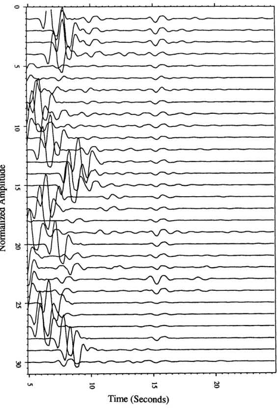
To test the performance of the simulated annealing teleseismic phase identification method, we apply the technique to synthetic data contaminated with various levels of noise and attempt to locate the Moho reflection in the synthetic data. We calculate synthetic seis-mograms for 30 different random earth models shown in Figure 3 using the source pulse shown in Figure 4. The random nature of the models is controlled to mimic probable crustal velocity profiles found in New England and the number 30 was selected as the minimum number of recording stations used in the New England study. We then test four different cases: first without noise, then with 10, 30 and 80% noise (actual ground noise recorded on the NEUSSN normalized to the peak of the synthetic trace). The synthetic data are presented in Figures 5, 6, 7 and 8.

The procedure outlined above is applied to the synthetic data to determine the relative two-way arrival times of the Moho, and the results of these tests are shown in Table 1. From the first test we see that without noise we can easily isolate the reflection to 0.1 seconds (1 sample). However, we also see that for 2 cases (Traces 29 and 30, which correspond to Models 29 and 30 of Figure 3) we get relatively poor travel time estimates. We conclude that this method has difficulty when the targeted discontinuity is represented as a gradational velocity change; for Models 29 and 30 little or no PmP energy exists. Figure 9 shows the noise-free data after the final lags are applied to each trace and the PmP phase is clearly located. We see from the final trace stack (Figure 10a) that in addition to estimating most of

(31)

the reflection times, we have also determined the source wavelet used to create the synthetic data (with polarity of the PmP phase reversed from that of the direct P). As the noise level is increased to 10% (Table 1 and Figure 10b), the results are still good, with only the last two trace lags poorly defined. As we increase the noise to 30% (Figure 10c) and to 80% (Figure 10d) the results are degraded. At 80% the usefulness of the method is questionable, with inaccurate estimates (greater than 0.4 seconds error) in over half of the traces. We conclude that noise levels above 50% can degrade the results to unusable levels. Fortunately, network seismic data are sufficiently abundant that we can select many waveforms with good

signal-to-noise levels (below 30%) .

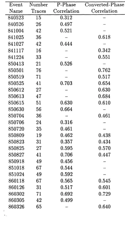
One other obvious limitation of this method is that it requires some knowledge of the window (the travel times to the targeted phase in the data) before the method can be applied, ie; we must have a good estimate of the the arrival prediction window to insure that an arrival which is not targeted in the application is not interpreted as the correct arrival. We also must assume that the arrival exists, because this method will find the best possible lag in the prediction window even if there is no actual arrival at all (Trace 29, for example). To overcome these problems, we save the maximum trace correlation level between the prediction window and the annealing stack reached at each station during the procedure as a measure of the performance of the optimization procedure at each station. For example, in the NEUSSN Moho application we apply the simulated annealing method to numerous teleseismic data sets (waveforms recorded on the NEUSSN) and from each data set we derive a Moho travel time estimate at each station. We use the maximum trace correlation values as weighting factors in the final estimate of the Moho travel time at each station. For the synthetic tests, the maximum trace correlation values are included in Table 1 and we see that the final peak trace correlation between the target window and that in a few cases even the best stack can be quite variable even when noise is absent. In the noise free-case the peak trace correlations are almost all very good, where we see that only the velocity-gradient cases have peak trace correlation values less than 90%.

To examine the usefulness of the final peak trace correlation value (between the trace window and final annealed stack) as a measure of a parameter estimate quality factor, a

(32)

quantity we will use below to weight our travel time estimates, for each test model we plot the difference between the actual relative travel time and the predicted relative travel time versus peak trace correlation level. These plots (Figure 11) are shown for the noise free case, as well as the 10, 30, and 80% noise cases. We see that for the noise free example all peak trace correlations from models with strong Moho discontinuities are high (greater the 0.9), but as noise starts to dominate (30% and 80%) we see that the models with high travel time errors generally have smaller trace correlation values. For this reason, in the applications

below we weight each Moho travel time estimate by the maximum trace correlation level. A second weight is applied to the Moho travel time estimates. We use the maximum correlation between the final annealing stack and the effective source wavelet for the event (see Chapter 4) to reflect the overall quality of the estimates from each event in the analysis. This correlation level is referred to as the event correlation level. When the waveforms are shifted to optimize the power of the annealing stack (the objective function) the resultant wavelet should duplicate the source pulse (inverted due to the negative reflection coefficient). If we assume that the stack of the direct phases represents the source wavelet (discussed Chapter 4), then the event correlation should provide a good event-wide weighting factor. So, as a final estimate of Moho travel times at an individual station we determine the travel time with the simulated annealing procedure and weight this value by the product of the peak trace correlation level and the event correlation level.

2.4 Implementation Issues

Event Selection

For the New England Moho application, earthquakes were selected with consideration given to epicentral distance, event depth, source signature complexity, source duration and signal-to-noise ratio. We use events with well defined effective source signatures (Chapter 4), so that we can evaluate the overall performance of the method for each event by correlating the effective source with the wavelet reconstructed from the tar-geted reflector. All of the events used in both New England and Larderello applications have relatively sharp and simple waveshapes. Many of the available events were not

(33)

included in the annealing analysis because of excessively long durations of the source wavelets.

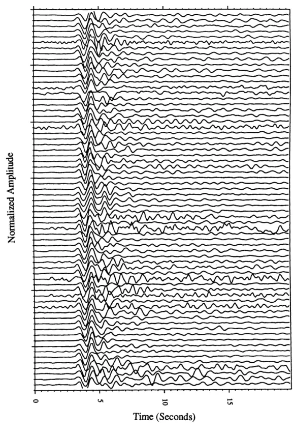
As an example of the data used, we show in Figure 12 waveform data for a typical event recorded on the NEUSSN: the May 1, 1985 earthquake of Peru, hereafter referred to as event 85/05/01. In this plot the natural direct P-wave moveout is removed using the simulated annealing technique. The data show a coherent initial source pulse but little visible similarities in any of the later phases.

* Phase Selection

For events with teleseismic distances in the range of 40-180 degrees, reflections from discontinuities deep in crust generally arrive at a station between 5 and 15 seconds after the direct P-wave and with incidence angles between 50 and 0 degrees from vertical. These arrivals have amplitudes generally less than one tenth of the direct arrival. For a horizontally stratified media, the delay of reflected arrivals is dependent on source-receiver distance, crustal thickness and average crustal velocity. At steep incidence angles (less than 30 degrees from vertical) the P-waves dominate the waveforms, while at shallower angles (greated than 30 degrees) S-energy dominates. (See Chapter 5 for a description of the amplitude and travel time dependence of crustal phases with various incidence angles). To take advantage of this phenomenon we target P-wave reflections for steeply arriving events and converted-phases (one leg of the reflection is a P-wave, one leg is an S-wave) arriving at more oblique angles of incidence.

* Conversion to Absolute Travel Times

The simulated annealing method is applied separately to each event. After a suite of trace shifts which maximize the stack power are determined, we calculate the relative delay for each station included in the event. This procedure is followed for all events and then the results from a particular station are combined and interpreted to produce a single measure of the relative 2-way travel time to the discontinuity beneath each station. To convert the relative times to absolute estimates of 2-way travel time, we select a few stations in the network as control areas where the velocity structure is

(34)

well known from previous studies. The relative values are time shifted until they best match the estimates of the inferred vertical two-way travel time of the control areas. For the New England analysis we have good deep crustal information in Central Maine (Leugert, 1985; Kafka and Ebel, 1989) and eastern Massachusetts (Foley 1984; Doll, 1987).

* Error Analysis

With the simulated annealing technique noise-free traces can be aligned to a precision of a single sample, and with the sampling rate set to 10 samples per second, our alignment precision is 0.1 second. For a typical crustal propagation angle of 25 degrees and an average crustal velocity of 6.6 -, a 0.1 second error in alignment corresponds to 0.3 km error in interface depth estimation. When noise is introduced, timing accuracy is degraded, so 0.3 km represents the best possible depth resolution of an interface. In the real data applications we make several estimates of the vertical two-way travel time at each station (one for each event in the analysis), and we calculate the average travel time and variance for each station. The variance is used to guide the interpretation of the results and is discussed below. In general, the variances in vertical travel time estimations are about 0.3 seconds, corresponding to a resolution in crustal thickness of about 2 km. Errors in average crustal velocity estimates produce errors in depth estimates when converting travel time estimates to depths. For example, for a ray traveling 25 degrees off vertical, the Moho depth estimate made from a PmP travel time estimate of 10.0 seconds is in error by 0.5 km when the estimate for average crustal velocity is in error by 0.1 km/sec. Given that the highest frequencies observed in our teleseismic P-waveform data are about 3 Hz, the the shortest wavelengths observed are about 2 km and errors of magnitude 0.5 km cannot be resolved in the data.

* Conversion Temperature

The conversion from cross correlation to probability distribution is very important in the simulated annealing method (Rothman, 1986). We tested three different con-version cases: no annealing (T = 0; conventional cross-correlations), steady state annealing (T = constant for all iterations) and temperature varying annealing (T =

(35)

To [1 - cooling rate]iteration). For event 85/05/01 the calculated stack power histories

for the three different methods is plotted in Figure 13. The final stack power level

for the case where T = 0 (no annealing) is lower than both the constant

tempera-ture and iteration dependent annealing results. This indicates that the probabilistic approach to teleseismic arrival time selection is an improvement over a simple cross-correlation technique. We also see from the stack power plots that both the steady state and iteration-varying applications reach an equal stack power level and that the temperature varying procedure takes about 5 times as many iterations to reach this level. However, it must be realized the conversion temperature used in the steady state case was determined with a careful and time consuming trial-and-error process. The temperature is a sensitive parameter, and a 10% change in starting temperature can cause the procedure to get trapped in local minima. By implementing a scheme where temperature varies with iteration, a wider range of starting temperatures can be used. We significantly reduce the importance of the starting temperature and therefore auto-mate the process. The tradeoff of this implementation is that the number of iterations necessary for the procedure to converge is increased. We find that in most cases we see convergence within 30-150 iterations. This convergence is quite rapid in contrast to the 3500 iterations Rothman (1986) needed to anneal data for static corrections. The relatively small number of iterations required in this teleseismic application indicates that global minima can be easily reached with the application of this probabilistic ap-proach to travel time picking and that the problem is not strongly contaminated with local minima.

2.5 New England Applications

The topography of the Moho discontinuity beneath the Northeastern United States Seismic Network (NEUSSN) is determined in this section by means of calculating the relative timing of Moho reflections across the region from numerous teleseismic events. We use the simulated annealing technique to determine the delay times of the Moho reflection (P,P) and to measure the confidence of each travel time selection.

Crustal structure from teleseismic bodywave data

Crustal Structure from Teleseismic Bodywave Data

by

John Edward Foley

M.S., Boston College (1984)

B.S., University of Lowell (1981)

Submitted to the Department of Earth, Atmospheric, and Planetary

Sciences

in partial fulfillment of the requirements for the degree of

Doctor of Science

at the

MASSACHUSETTS INSTITUTE OF TECHNOLOGY

June 1990

@

Massachusetts Institute of Technology 1990

All rights reserved

Signature of A uthor ...

.... . ....

... .. .. ....

...

Department c Earth, At

heric, Qd Planetary Sciences

SMay

25, 1990

Certified by.

(

Accepted by...

..

9

M. Nafi Toksiz

Professor of Geophysics

Thesis Advisor

Thomas H. Jordan

Chairman

Department of Earth, Atmosphgc,

and Planetary Sciences

'*~--Crustal Structure from Teleseismic Bodywave Data

by

John Edward Foley

Abstract

Acknowledgments

Contents

Chapter 1

INTRODUCTION

1.2 The Larderello Geothermal Region

1.3 Introduction to the New England Application

1.4 Roadmap and Description of Methods

]

[]

SDevonian

Chapter 2

SIMULATED ANNEALING WITH

TELESEISMIC DATA

2.1 Introduction

2.2 Simulated Annealing Method

e

C

(

C

2.3 Synthetic Examples

2.4 Implementation Issues

2.5 New England Applications

**'*~--Crustal Structure from Teleseismic Bodywave Data**