HAL Id: in2p3-00178042
http://hal.in2p3.fr/in2p3-00178042
Submitted on 26 Oct 2007HAL is a multi-disciplinary open access archive for the deposit and dissemination of sci-entific research documents, whether they are pub-lished or not. The documents may come from teaching and research institutions in France or abroad, or from public or private research centers.
L’archive ouverte pluridisciplinaire HAL, est destinée au dépôt et à la diffusion de documents scientifiques de niveau recherche, publiés ou non, émanant des établissements d’enseignement et de recherche français ou étrangers, des laboratoires publics ou privés.
GLAMPS - Analysis Package for GANIL Data and
Application to VAMOS-EXOGAM Experiments
Avhishek Chatterjee, P. Sugathan, A. Navin, M. Rejmund
To cite this version:
Avhishek Chatterjee, P. Sugathan, A. Navin, M. Rejmund. GLAMPS - Analysis Package for GANIL Data and Application to VAMOS-EXOGAM Experiments. 2007, pp.1-21. �in2p3-00178042�
GLAMPS
Analysis Package for GANIL Data and
Application to VAMOS-EXOGAM
Experiments
A.Chatterjee*, P.Sugathan, A.Navin, M.Rejmund
GANIL, BP 55027, F-14076 Caen Cedex 05, France
*Present address: Nuclear Physics Division, BARC, Mumbai 400 085, India Email: [email protected]
1 Introduction 3 6.1 Introduction to VAMOS 11 2 Obtaining the package 3 6.2 Employing user.F for
VAMOS data
14 3 Before you install 3 6.3 6.3 Editing BSTART 14 4 Installation 5 6.4 6.4 Subroutine USERSUB 16 4.1 Installing the help files 5 6.5 Subroutine DRIFT 16
5 Basic steps in using the package
5 6.6 Subroutine
RECONSTRUCT
17 5.1 Locating the list files 6 6.7 Subroutine
ION_CHAMBER
17 5.2 ACTIONS_local.CHC_PAR 6 6.8 Subroutine SI_WALL 17 5.3 Fine tuning the ACTIONS file 8 6.9 Subroutine
IDENTIFICATION
18 5.4 Preparing the Setup 9 6.10 Subroutine EXOGAM 18 5.5 Editing user.F 10 6.11 Subroutine FSTOP 18
5.6 Analysis 10 6.12 Sample plots 19
5.7 Analysis Functions 11 7.1 Rewriting List Files 21 6 The VAMOS Spectrometer 11 8 Conclusion 21
1. Introduction
Experiments in nuclear reactions and spectroscopy at accelerator laboratories such as GANIL acquire large amounts of data (typically 10-100 Gb). During the experiment one- and two- dimensional spectra of the raw as well as derived parameters can be displayed in the online acquisition system VISUGAN. Complete analysis is usually done offline. Since the data collected is available on disk, it is possible to begin the offline analysis even while the experiment is in progress and this can help to notice problems and improve the experiment. In this report we present a short write up about the GLAMPS [1] package for the offline sorting of data. The package is simpler to install and use compared to ROOT [2] and is ideally suited for quick offline analysis. It works with the GANIL data directly and no format conversion is needed. It is completely driven by an intuitive menu interface and there is no command line. Using the software does not require a substantial learning time. Most of the common tasks are built-in. A user program (user.F) can be written and linked into the code as well. A sample user.F code for VAMOS-EXOGAM experiments is provided and explained in this report as an example. The code for GLAMPS is written in C. The user code (user.F) is normally written in FORTRAN (but could also be written in C or C++ if desired). GLAMPS must be installed under Linux. It is also known to work in Windows under Cygwin [3] (contact the author in case of problems). At this time it is not supported on Mac OS X (however you can run GLAMPS in Linux on a Mac).
2. Obtaining the package
The GLAMPS package is available at the LAMPS website (Pelletron Laboratory, Mumbai, India) http://www.tifr.res.in/~pell/lamps.html (a link is also provided at the GANIL website: http://www.ganil.fr). You should download the following files:
File Approx Size
1 glamps28-03-07.tgz
(version date subject to change) 192 Kb
2 help.tgz 908 Kb
Both files are tar-gzip archives. The first file contains the source code of GLAMPS; the second contains the help files in html format. The help files actually pertain to LAMPS (data acquisition program at Pelletron Laboratory, Mumbai) and not to GLAMPS. However many features of GLAMPS are the same as those in LAMPS.
3. Before you install
Compilation of GLAMPS needs the C compiler, FORTRAN compiler and the graphics library gtk-1. The C compiler gcc is to be found on all Linux installations. The Makefile for GLAMPS assumes g77 as the Fortran compiler. However, in some computers the name of the FORTRAN compiler could be different (e.g. gfortran). In this case edit Makefile accordingly. GLAMPS
uses only very common features of C and FORTRAN, so the compiler version does not matter. The graphical library gtk-1.x is used by GLAMPS. You need not only the runtime package gtk+-1.2 but also the development package gtk+-devel-1.2. The following 4 packages are required by GLAMPS:
glib-1.2.10-23
glib-devel-1.2.10-23 gtk+-1.2.10-55
gtk+-devel-1.2.10-55
(The version numbers 10-23 or 10-55 are not important, any version will do)
The first thing to do is to check if you have these packages already installed in your computer. To check this you don’t need root permission. Type the following commands:
$rpm –qa | grep “gtk” $rpm –qa | grep “glib”
Note that you need gtk1 and glib1, (not gtk2 and glib2). If you don’t have these 4 packages you need to download and install them (If you don’t have root permission, ask the system administrators to install them). These packages are small and on a system where gtk2 is already installed, additional installation of gtk1 does not cause any conflict. For your convenience these files are made available at the lamps website – click “Compiling under Fedora Core 6” on the main page
(http://www.tifr.res.in/~pell/lamps_files/htm/FedoraCore6.htm).
The files compatible for Fedora7 are provided in the link “Compiling under Fedora 7”. If you are running a recent version of Ubuntu Linux or Scientific Linux you can safely use the files corresponding to Fedora Core 6. Alternatively, a search on http://rpmfind.net allows you to download rpm files compatible with your version of Linux.
To install the packages use e.g. the following command as root: #rpm --install glib-1.2.8-1.i386.rpm
The screen resolution best for GLAMPS is 1280x960. With 1024x768, the main display windows will be okay but the Parameter List window will be partly covered. Higher resolutions are no problem -- only the top left part of the screen will be used. To know your current display settings or change them (if you have the GNOME desktop) click on “Desktop:Preferences: Screen Resolution”.
In recent versions of Fedora the Linux task bar is split into two and located at the top and bottom of the screen. This is not a friendly configuration for GLAMPS. To correct this problem, before starting GLAMPS, click and drag the top half of the task bar and relocate it at the bottom of the screen.
4. Installation
In the description below we use the name glamps28-03-07.tgz for the downloaded file. (The actual version date will change). Create a folder, e.g. glamps. (If you are working on several experiments, make a separate installation for each experiment). Copy glamps28-03-07.tgz here and unpack it:
$tar zxvf glamps28-03-07.tgz
This will create several directories (see Section 5 below) including a src directory. Go to the source directory (src) and type make. You should not get any errors or warnings. If you do, it could be due to a differing Linux version (please send mail to [email protected] or [email protected] to correct the problem). The only known warning is about unused variables in the user.F file which happens when you have not yet edited user.F for serious use. To run the program, go back to the top level directory and follow the steps detailed in Section 5 below.
4.1 Installing the help files
The help files form a completely independent package. After unpacking, the help files can be viewed with a web browser. Copy the file help.tgz to any directory of your choice. Unpack it with the command
$tar zxvf help.tgz
Double clicking index.html will open the html files.
5. Basic steps in using the package
Go back to the top level directory (e.g. glamps): $cd ..
Now you are ready to run the program. (The executable files are located in the exe directory. You don’t need to copy them here.)
$glamps (or ./glamps if you don’t have ./ in your path)
It is desirable to include ./ in your path. If you are using the bash shell, edit the hidden file .bash_profile in your HOME directory and add ./ to your PATH. Change PATH=$PATH:$HOME/bin to PATH=$PATH:$HOME/bin:./
The new PATH takes effect when you login again.
Subdirectory What it holds
Top level ACTIONS_local.CHC_PAR (see Sec 5.2) Calibration files for VAMOS (see Sec 6.3) src Source codes and Makefile
src/userF Collection of user.F files set Setup files (initially empty) bat Batch files (initially empty) ban Banana gate files (initially empty) cal Calibration files (initially empty) exe All the executables
dat Sample VAMOS calibration files
5.1 Locating the list files
During acquisition at GANIL, the data files are written to a shared RAID disk mounted as /data with a subdirectory name corresponding to the name of your experiment, for example /data/e514X/exodiam/acquisition/run
Often a second copy of the data is acquired on an external USB disk.
If you are working on data while the experiment is in progress, you can access files directly from /data. It is possible to start GLAMPS for a file where acquisition is still going on, but normally we run GLAMPS for files whose acquisition has been completed. The batch file feature of GLAMPS allows you to analyse many runs together.
If you are analysing data after the experiment and are outside the GANIL network you can work with a copy of the data files.
The data file names are of the form run_nnn.dat.date.time where nnn is the run number (E.g. run_0515.dat.06-Sep-05.02:33:13). These long file names with multiple dots do not cause any problem in running GLAMPS and it also works fine if you rename the files as run_nnn.dat. GLAMPS can rewrite list files, deleting unwanted parameters, adding new derived parameters and/or filtering the events (for details see Section 7.1). In this case you should maintain .dat in the new file names.
5.2 The ACTIONS_local.CHC_PAR file
The first thing to worry about is the ACTIONS_local.CHC_PAR file. If you don’t already have it in your working directory, GLAMPS cannot proceed (however GLAMPS can generate this file: see below). The ACTIONS file is created during acquisition. It is a text file containing the parameter list with 3 columns: Parameter name, VME Address and ADC Bits. Here is an example showing a few lines of this file:
GATCONF 257 8 TSED_HF 1297 14 TSI_SED 1809 14 TSED_GAMMA 0 13 TSED_MCP 0 13 TSI_HF 1041 14 TSI_GAMMA 261 14 PILEUP 5 14 ECC_13_A 7953 13 ECC9_A 517 13
If you do not have this file in your working directory, you will see the message:
If you don’t know where to find this file, GLAMPS can generate it for you by looking at a typical list data file. After GLAMPS starts, click on Utilities: Make ACTIONS File as shown in the picture below and select Browse to select one of the .dat files.
After ACTIONS_local.CHC_PAR has been created, you should exit GLAMPS and start again. You will now see the parameter list in its own window to the right of the screen.
5.3 Fine tuning the ACTIONS file
For many purposes the ACTIONS_local.CHC_PAR file constructed as above or copied from the acquisition directory is sufficient. However it is not optimal. A big ACTIONS file with parameters that are not needed in the analysis is wasteful. Faster running of GLAMPS will be ensured by eliminating the lines in the ACTIONS file that are not needed. There is also another reason to fine tune the ACTIONS file. You may prefer to rearrange the order of the parameters. For example, if you already have a working user.F in a VAMOS-EXOGAM experiment and now you are moving onto a VAMOS-INDRA experiment you may like to have the VAMOS parameters listed first followed by the INDRA parameters.
A program actions.c is provided within the GLAMPS archive which helps you to fine tune the ACTIONS file. (Its use is optional, you can start GLAMPS without fine tuning, or you can edit the ACTIONS file yourself). First you need to compile the actions.c file (It is not part of GLAMPS, and the make command does not compile it):
$gcc actions.c -o actions
The program actions works by taking the original ACTIONS file (which must be renamed as ACTIONS_original.CHC_PAR), comparing it with a file called ActionsTemplate.list (which the user must prepare himself) and produces the fine tuned file ACTIONS_local.CHC_PAR. An example of ActionsTemplate.list is given below:
#ACTIONS TEMPLATE FILE for Vamos-Exogam experiment 27/10/2006 #Example: ECHI_[A-C]_[1-7] (A-C:outer loop, 1-7:inner loop)
001 GATCONF 002 TSED_HF 003 TSI_SED 004 TSED_GAMMA 005 TSED_MCP 006 TSI_HF
007 TSI_GAMMA 008 PILEUP 009-058 Extra_[1-50] 059-060 TFIL_[1-2] 061-062 EFIL_[1-2] 063-126 STR_11_[01-64] 127-190 STR_12_[01-64] 191-254 STR_21_[01-64] 255-318 STR_22_[01-64] 319-339 ECHI_[A-C]_[1-7] 340-360 SIE_[01-21] 361-404 ECC[2-12]_[A-D]_6MEV 405-448 ECC[2-12]_[A-D]_20MEV 449-624 GOCCE[2-12]_[A-D]_[0-3]_E 625-668 ECC[2-12]_[A-D]_TAC 669-679 ESS[2-12]_TDC
Each line has two fields. The first is the parameter range and the second is the names of the parameters. (The number in the first column is for your own reference, the program does not check its value). The first line 001 GATCONF means that GATCONF will be parameter number 1. The line 063-126 STR_11_[01-64] means that STR_11_01 will be parameter 63, STR_11_02 will be parameter 64 and so on. The line 449-624 GOCCE[2-12]_[A-D]_[0-3]_E means that GOCCE2_A_0_E is parameter 449, GOCCE2_A_1_E is parameter 450, ... GOCCE3_A_0_E is parameter 453 etc. When actions is run, it compares ActionsTemplate.list with ACTIONS_original.CHC_PAR and picks up the VME addresses to construct a new ACTIONS file called ACTIONS_local.CHC_PAR.
5.4 Preparing the Setup
You can start analysis of a file without preparing a setup (in this case 1d spectra of all the parameters appearing in the ACTIONS file will be built), but usually a setup is prepared. Click Setup: Edit Setup and input the number of spectra 1d and 2d that you wish to build. The Define button allows you to specify the parameter numbers and gating conditions for each spectrum. In addition you have to specify the number of Pseudo parameters and their definitions. Pseudo parameters are parameters obtained by mathematical constructs on the original parameters. If there are 680 (real) parameters then the first pseudo will start at 681 in the parameter space. From then on, you can refer to this pseudo either as Pseudo 1 or as Parameter 681. There are a number of pre-defined pseudos (Sum, Product, Ratio, Position, PI, Multiplicity, Array, BGated, TOF_E), and you can define your own pseudos in user.F. The VAMOS example detailed in the next part of the report constructs all the required pseudos in user.F and does not use any of the built-in pseudos.
After preparing the setup, save the file in the directory set located below your working directory (an empty set directory would have been created during installation). The next time you start GLAMPS it remembers the setup file you were last using and loads it automatically. So
you don’t need to go through the process of loading a setup file every time unless you want to switch between multiple setup files.
While defining spectra, parameter number zero refers to a hit pattern spectrum. A hit pattern spectrum is useful to show e.g. which parameters are not firing at all.
There is also the possibility to build vector spectra. A vector spectrum is one for which the parameter is given a range of values. For example if parameter numbers 300 to 315 are the add- backs of a 16-clover array, then specifying 300:315 builds the spectrum of the entire array. In this case, if in an event more than one detector has fired, the channel number is taken from the detector coming first in the range 300:315. For vector spectra all the parameters specified must have the same resolution. Similarly one can build vector-vector 2d spectra, in which both the X and Y axes are specified as a range of values. Gamma-gamma matrices can be built in this way.
5.5 Editing user.F
If you are constructing parameters in user.F (see the detailed example for VAMOS in the next section) you need to edit the user.F file and recompile. Go to the src directory below your working directory and edit user.F. After you have finished, make a copy of user.F with a name like user-vamos-01-May-2007.F and move it to src/userF to preserve as a backup. (As you work with GLAMPS you will find yourself developing many versions of user.F, it is easy to get confused, so do keep a record of your work.). After that a make command executed from within the src directory will compile the new user.F and link it. If you get any errors or warnings, correct these and do make once again.
5.6 Analysis
To start analysing data click Analysis: Start. You see an Offline Analysis window. Click Add then Browse to add all the files you want to analyse.
By default, spectra are cleared (zeroed) at the start of the analysis of a batch of files, and after that, they acquire statistics from all the runs. (See the entries in the second column Zero
Spec). It is possible to read entire files (default) or skip part of the file (see last column). In general, the list of files to be analysed could be quite big. You don’t want to manually add them every time. You can save the list by clicking Save Batch File. Save this to the directory bat which was created as an empty directory during installation. Additionally, even if you don’t save the Batch File, GLAMPS remembers the last used set of runs and loads them automatically when you restart GLAMPS.
(It is important to organise your files into directories like this. Each time GLAMPS is restarted it remembers the directories for file types and the file browser redirects itself, so please do not scatter your files in arbitrary directories to avoid trouble later on).
On clicking Start Analysis the analysis starts and the status in the main GLAMPS window shows the progress.
5.7 Analysis functions
The program has a rich set of analysis features. One can find more information about these features by browsing the help package. Notable features worth mentioning:
Calibration: Single click calibration of Ge spectra for standard sources like 60Co, 152Eu
Banana Gates: Polygonal gates can be drawn in 2d spectra and saved for later gating. The polygon can be repositioned, rotated or scaled by the user.
Multi-Peak Fit Analysis: Spectra can be fitted to multi-Gaussian functions with tail and asymmetry parameters to extract yields
Rewriting List Files: GLAMPS includes an interface to construct new list files including new parameters and deleting unwanted parameters (see Section 7.1)
The user interface for these features is completely intuitive and does not require detailed explanation (Refer to the downloaded help.tgz if necessary). Regions of interest are selected by left-mouse drag and all the functions are accessible by right mouse click over a spectrum window.
6. The VAMOS Spectrometer 6.1 Introduction to VAMOS
VAMOS (Variable Mode Spectrometer) is a large acceptance mass spectrometer [4-6] operational at GNAIL since 2002. It has been widely used in many experiments for identifying the products in nuclear reactions using both radioactive ion and stable beams from GANIL. Coupled with high efficiency gamma detector arrays like EXOGAM, the spectrometer provides a sensitive and high performance tool for detecting and studying the spectroscopy of exotic nuclei produced in deep inelastic, transfer and fusion- evaporation reactions.
Fig 6.1.1 Schematic of VAMOS Spectrometer
The ion optical elements of VAMOS consist of a pair of quadrupoles (Q), a velocity filter (F) followed by a magnetic dipole (D) in the configuration, Q1-Q2-F-D. The dispersion at the focal plane can be varied by changing the bending angle of the dipole with three options of 0, 45 and 60o bending. The velocity filter allows the use of the spectrometer as a recoil separator for zero degree operation. Further, the spectrometer has the flexibility to be rotated with respect to the beam direction in the angular range 0-60o and the distance between target and first quadrupole can be varied. The spectrometer is supported on a platform which can be moved outward to change the distance from the target and this platform in turn rests on another platform on rails allowing rotation around the target point. These flexibilities make VAMOS a unique device as variable mode spectrometer.
The rotating platform extends upstream for the placement of an ancillary detector system like EXOGAM. When EXOGAM array is coupled to VAMOS and the platform is rotated, the EXOGAM array also rotates about the target point and the relative angle between VAMOS and EXOGAM stays the same.
Fig 6.1.2 Schematic of the VAMOS focal plane detection system showing the focal plane and the coordinate system
The detection system at the focal plane of VAMOS consists of different sets of detectors adapted to the kind of experiments involved. For light and fast ions the position X, Y and angles, θ, φ of the trajectory are measured using a pair of drift chambers (DC). These detectors are gas based vertical drift chambers consisting of a cathode plane, Frisch grid, amplification wires and anode plane. The anode plane is segmented into 128 pads in two rows (64 pads in one row). The ions passing through the gas create electrons which are accelerated to the wires where they get amplified and induce charges on the anode pad. The charge from each pad is collected and processed through GASSIPLEX electronics. The pad signals give the horizontal position X, and the vertical position is extracted from the drift time of electrons reaching the amplification wires. Typical resolutions of 0.5mm in X and 1 mm in Y are expected. The two drift chambers (DC1 and DC2) are kept at a separation distance of 1 meter. The drift chamber signals provide the set of focal plane trajectory coordinates (X, Y, θ, φ).
In the case of slow heavy ions, detectors based on secondary electron detection (SED) are used for position and timing information. A pair of large area SEDs gives X, Y position and fast timing. The SED can give time resolutions of the order 250 ps. This detector consists of a thin aluminised mylar foil which emits secondary electrons when hit by particles. The secondary electrons get accelerated and amplified in a position sensitive gas detector.
For the purpose of reconstruction, a fixed plane midway between DC1 and DC2 is visualized as the focal plane (Fig 6.1.2). The processed values of X, Y, θ, φ refer to positions and inclinations of the detected trajectory on this plane. Note that θ, φ are not conventional polar coordinates but horizontal and vertical inclination angles. Note also the use of two different
laboratory coordinate systems. The trajectories are followed in what will be referred to as ZGOUBI coordinates consisting of (X, Y, θ, φ). After completing the reconstruction of the event we obtain the target variables Bρ, θT, φT and path length (Δ). From these, one can
compute the polar angles θL, φL of the trajectory with respect to the beam direction.
The measurement of mass of the detected particle requires the measurement of time-of-flight (TOF) to good precision. For mass and particle identification, the time of flight TOF, energy E and energy loss ΔE are measured. The time of flight between the target and focal plane is recorded using start detector like MCP or RF of accelerator. The energy loss ΔE and energy E measurement is done using segmented ionization chamber IC and silicon wall detector. The IC consists of segmented anode with 21 pads (3x7) followed by an array of 21 Silicon detectors. Since VAMOS is a large acceptance spectrometer, direct focal plane measurements alone do not give the required high resolution identification. Particle identification is based on the reconstruction of the event. The scattering angle at the target and Bρ parameter is reconstructed in software. For this purpose, the ion-optics program ZGOUBI [7] is employed before hand to prepare 7th (or higher order) polynomials allowing the variables Xf, θf, Yf, φf to be transformed
to the target variables Bρ, θT, φT and path length (Δ).
Velocity of the particle is deduced from the time of flight and path length and M, Z, E identification is achieved from Bρ, TOF and ΔE.
6.2 Employing user.F for VAMOS data
The GLAMPS package includes the file user-vamos.F to be found in the directory src/userF. Make a copy of user-vamos.F renamed as user.F in the src directory (overwriting user.F to be found here). On executing the make command in the src directory, the code relevant for VAMOS is compiled and linked. While using GLAMPS the process of editing user.F and recompiling, may be required many times. Therefore it is useful to save versions of user.F with appropriate names in the directory src/userF. In studying the information below it is essential to keep a listing of the user-vamos.F code handy. Most of the documentation is to be found in the form of comments inside the source code. The code listing is 12 A4 pages (about 700 lines).
6.3 Editing BSTART
To begin with, the user must go through the subroutine BSTART and edit it as required. BSTART is called at the beginning while analysing a set of files and it includes a number of variables that need to be set correctly.
!Parameter placements: Depends on VamosTemplate.list
ID_P=63 !Parameter number of STR_11_01 ID_T=59; ID_E=61 !Parameter number of T_FIL1 and E_FIL1 ID_I=319 !Parameter number of ECHI_A_1 ID_SI_E=340 !Parameter number of SIE_01 ID_SI_T(1)=6; ID_SI_T(2)=3; ID_SI_T(3)=2; !Para number of TACs ID_6MEV=361 !Para number of ECC2_A_6MeV (first clover) ID_20MEV=405 !Para number of ECC2_A_20MeV (first clover) ID_GOCCE=449 !Para number of GOCCE2_A_0_E (first clover) ID_ESS=669 !Para number of ESS2_TDC (first clover)
The parameter list is to be found in the file ACTIONS_local.CHC_PAR (Section 5.2). If possible, the order of the parameters in this file should be changed making use of the template file VamosTemplate.list in the way described in Section 5.2 to conform to the above numbering. Otherwise, one can edit the above lines suitably. In the above example ID_P=63 specifies that the drift chamber outputs STR_11_01 … start from Parameter 63 (and continue sequentially). Similarly important are the other parameter placements. GLAMPS works with parameter numbers, once the parameter placements have been correctly specified as above. The next line specifies the angle of the spectrometer (The example below shows 35 degrees, edit as needed):
VAMOS_ANGLE=35./RA_DG
After that, BSTART() reads information from 6 files. It is required that the user prepares and makes a copy of these calibration files in the top level directory from where glamps is being run. As a starting point, you will find suitable files in the dat directory.
1 DriftChamber.cal Calibration parameters of the drift chamber 2 DriftChamberRef.cal Positions of the reference beam
3 Reconstruction.cal Contains BRHO_REF, names of 4 files and PATH_OFFSET 4-7 The four files referred
above
Each contains 330 coefficients for the 7th order polynomial. Used for reconstruction.
8 IonisationChamber.cal Calibration coefficients for the Ionisation Chamber 9 Si.cal Calibration coefficients for the 21 Si wall detector
10 glamps.cal Calibration coefficients for the EXOGAM array. This file can be generated by glamps by performing single click Eu source calibrations of the EXOGAM array. The file has then to be copied from the CAL directory to the working directory
11 GOCCE1.cal Theta and Phi of the EXOGAM segments 12 ESS_TDC_LIM.dat ESS limits for Compton rejection
The information contained in these files is to be obtained from mechanical measurements, source data and pencil beam measurements. Files similar to these are to be also constructed for online data viewing in VISUGAN or if you are analyzing with ROOT. To learn more about the actual parametes contained in these files, refer to the documentation included as comment lines
in the sample user-vamos.F file and the sample calibration files provided. The files are all in free format so do not require to be typed in specific columns.
Editing BSTART is usually not needed if the parameter order has been changed by the use of VamosTemplate.list. However the proper construction of the calibration files is essential. The remaining subroutines in user.F are described below. You will need to change according to the specific configuration of the VAMOS focal plane detector system.
6.4 Subroutine USERSUB
This is the subroutine that GLAMPS will call on an event-by-event basis. All events are routed through here. USERSUB in turn calls the subroutines for different focal plane detectors and the EXOGAM array. If a particular detector type is not used in your experiment, simply comment out the call to the relevant routine by adding an exclamation point (!) at the beginning of the line. Notice that all the calibration parameters that were read in BSTART are made available to USERSUB wit the help of COMMON blocks.
USERSUB constructs 130 pseudo parameters (parameters that are mathematically related to the raw parameters). The list of 130 pseudo parameters is documented as comment statements in USERSUB. The first four pseudos are the X parameters (X1 to X4) in the drift chambers. Notice the use of LCLIP to constrain parameter values to be inside desirable ranges. Without this precaution, GLAMPS may crash with a segmentation fault. From these LCLAMP statements the upper limit of each pseudo should be noted and used as the ADC gain in the GLAMPS setup, for example X1 to X4 are to be set to an ADC gain of 1024.
There are statements near the beginning of USER.F which will cause a quick RETURN for unwanted events. Check these carefully. At the early stages, when the calibrations are not yet finalised, the statements can be commented out. For example:
CALL SI_WALL(NADC,NSEUDO,ADC) ; IF (M_SI.NE.1) RETURN
This statement filters out all events that have a multiplicity other that 1 in the Si wall. If the Si wall is not (yet) calibrated one should comment out this line so that other parts of the code can be tested.
USERSUB is the place to introduce PRINT statements followed by PAUSE to make diagnostics. One should proceed with analysis only after verifying that the code and calibration for each detector type is working correctly. In the debugging phase, typically one introduces an early RETURN to bypass the rest of the code and checks the subroutines for each detector type.
6.5 Subroutine DRIFT
Subroutine DRIFT first calibrates the raw energy signals. A threshold of 300 channels is taken. This should be verified by displaying the raw spectra and corrected if required. Next, the subroutine computes X_FOCAL, THETA_FOCAL by locating the peaks in the calibrated
charge distribution (subroutine FINDPK). If FINDPK does not reject a bad event, subroutine HYP (with 2-dimensional Newton Raphson method) is used to effectively fit a hyperbolic functional form to the peak shape. The required interpolation is done by subroutine XFOCAL. The algorithm has been fine tuned for performance so that event-by-event analysis proceeds at reasonable speeds. There should be no need for the user to make any changes in the subroutines FINDPK and HYP.
The computation of Y_FOCAL and PHI_FOCAL is easier and does not involve a numerical algorithm. It is based on the TAC values T_FIL1 and T_FIL2. Correct the threshold value T_THRESH if required. The proper calibrations and drift velocity should have been entered in DriftChamber.cal for this.
The outputs of subroutine DRIFT are the four quantities X_F, THETA_F, Y_F, and PHI_F. These values get transmitted to USERSUB via the common block /FOCAL/.
6.6 Subroutine RECONSTRUCT
The drift chambers provide the values of X_F, Y_F, THETA_F and PHI_F. It is now possible to use the 7th order polynomial that has been fitted to the ZGOUBI output to make the event reconstruction. The coefficients are read from 4 files, named in Reconstruction.cal. Each file contains 330 coefficients. If a 9th or higher order polynomial has been employed, this subroutine (and the part in BSTART which reads the coefficients) can be modified appropriately. The outputs of this subroutine are the variables BRHO, THETA, PHI, and PATH. Additionally the rotation of the spectrometer with respect to the beam direction is taken into account (subroutine ROTATE) to obtain PHI_L and THETA_L. As already mentioned in Section 6.1, PHI_L and THETA_L are not zgoubi inclinations, but the actual polar angles of the detected ion with respect to the beam direction taken as z-axis.
6.7 Subroutine ION_CHAMBER
This subroutine computes the calibrated energies of the 21 ion-chamber pads making use of the values read from IonisationChamber.cal saving the results in the array E_IC(21). It also calculates the sum energy for the three rows A, B, C saving the results in the array ES_IC(3), the total of all 21 elements (ETOT_IC) and the multiplicity M_IC. These values are transmitted by the common block /IONC_OUT/. The user should have a look at the raw ion-chamber spectra first and decide a suitable threshold value (taken as 800 in the sample source code). The thresholds for the calibrated energies are in the file IonisationChamber.cal
6.8 Subroutine SI_WALL
This subroutine is also rather simple. It computes the calibrated energies (E_SI(21)), the Si-wall multiplicity M_SI, the sum energy ETOT_SI, the calibrated TAC values T_SI(1) to T_SI(3). The TAC values are the time signals in the Si Wall with respect to the beam pulsing system (HF) and the SED detector (if used) and also the time of SED with respect to HF.
Additionally, the subroutine also stores N_SI, the number of the Si detector that recorded a hit for multiplicity 1 events. In the final analysis, USERSUB will accept only events with M_SI=1 and N_SI will be the number of the Si detector that fired. The quantities that the user should check and change in this subroutine are the thresholds TRAW and ERAW.
6.9 Subroutine IDENTIFICATION
With the help of the information obtained in the focal plane detector elements and after reconstruction, we proceed to compute ΔE (PLE_DE) and total energy (PLE_E). PLE_DE is basically ETOT_IC plus corrections due to foils (one can also add the small energy loss in the drift chambers) and the total energy further includes ETOT_SI.
The time of flight will depend on whether an MCP was used for the start signal, or beam HF is taken. The stop could be the SED detector (if used) or else the Si wall. Accordingly the expression for D must be corrected. PATH refers to the trajectory length inside the spectrometer upto the point midway between the 2 drift chambers. If a SED stop detector is used, we need to account for its inclination (this is the expression coded in the sample program). If stop is taken from the Si wall, the additional distance to the Si wall should be addedd.
From the distance, D and TOF we now obtain the velocity, V (BETA=V/c and GAM are needed for Doppler corrections when using the EXOGAM array).
Finally from the energy PLE_E and the velocity, we obtain the mass, PLE_M. The quantity M/Q of the ion is obtained independently of the energy, form the reconstructed Bρ value and the velocity.
These quantities Mass and Mass/Charge are used to display identification plots. Typical plots are shown in Section 6.11. Critical to obtain the correct identification plots is to have good calibration values for all the parameters.
6.10 Subroutine EXOGAM
The EXOGAM array is often used in conjunction with VAMOS to obtain spectroscopic information of ions selected. The subroutine EXOGAM in conjunction with the subroutine EXO_SUM computes, for each clover the Doppler corrected add-back energy for both the 6 MeV and 20 MeV outputs. It takes care to add the energies of clover elements that are adjacent and sets E_=0 for diagonal scattering. The Compton suppression signal ESS is also used to reject events. For Doppler correction, the cosine of the relative angle between the gamma-ray and the particle is computed and used. This is done in terms of the dot product of unit direction vectors. The user should carefully check the EXOGAM geometry file GOCCE1.cal. It should correspond to the actual geometry employed in the experiment.
At the end of analysis of each file the code reaches here. This is the place where we can insert print statements to show file-by-file statistics. The code for FSTOP in the sample code prints out the total number of events (also displayed as millions of events), and the number of “bad” events, i.e. the events where reconstruction failed for different reasons.
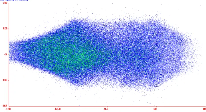
6.12 Sample plots
In this section we show typical plots. Fig 6.12.1 is from an experiment with 1.29GeV 208Pb on
70Zn target and the other two plots are from experiments with 1.2 GeV 238U beam on 58Ni.
Note that GLAMPS annotates the axes with floating point values making use of calibration values from glamps.cal.
Fig 6.12.1
This figure shows the final identification plot constructed as explained in Section 6.9. The best separation of the ions in this plot is obtained after all the calibrations have been done correctly.
Fig 6.12.2: THETA versus PHI is generated following reconstruction as outlined in Section 6.6. The pattern is illustrative of the acceptance of VAMOS in the settings used.
7.1 Rewriting List Files
One of the useful features of GLAMPS is the built-in interface for re-writing list files. Typically, the analysis procedure to extract information from an experiment is a long process lasting several months. If we are reading the same set of files repeatedly during analysis a lot of computer time is being spent on repetitive tasks. For VAMOS data after ensuring that the reconstruction procedure is working correctly, it is useful to rewrite the list files storing the reconstructed and derived quantities: BRHO, THETA, PHI, and PATH and/or PLE_DE,PLE_E,TOF,BETA,PLE_M,PLE_M_Q and abandon all the focal plane detector outputs. This will produce a much smaller list file and a major part of the analysis (VAMOS reconstruction) need not be done every time.
To rewrite files in GLAMPS: click Utilities: ReWrite List File. Before doing this one should have already prepared a suitable setup file and also linked up the user.F file capable of performing the VAMOS reconstruction. Now the interface presented allows parameters to be selected and deselected for the output file. One can process the files one by one or a set of files together, just as one does for analysis. The files generated will be again in the standard EXOGAM format common to GANIL data. However a new ACTIONS_local.CHC_PAR file has to be constructed (see Section 5.2) to read the new list files in GLAMPS.
8 Conclusion
In this short report it has not been possible to include every possible detail. Detailed information about the analysis features of GLAMPS can be obtained from the downloaded file help.tgz. The material presented here and the program GLAMPS are under regular revision. Later versions of this report and the latest version of the program will always be found at the LAMPS web site [1].
References
[1] LAMPS http://www.tifr.res.in/~pell/lamps.html [2] ROOT http://root.cern.ch
[3] CYGWIN www.cygwin.com [4] http://www.ganil.fr/vamos
[5] H.Savajols and VAMOS Collaboration, Nucl. Phys. A654, 1027c (1999).
[6] P.Sugathan, M.Rejmund, A.Navin, W.Mittig and S.Bhattacharyya (to be published); P.Sugathan, A.Chatterjee, B.Jacquot, A.Navin, M.Rejmond, EMIS Conference and Nucl. Instrum. Meth. (to be published).