The Impact of Sample Volume in Random Search on the bbob Test Suite

(1)

HAL Id: hal-02171213

https://hal.inria.fr/hal-02171213

Submitted on 2 Jul 2019

HAL is a multi-disciplinary open access

archive for the deposit and dissemination of

sci-entific research documents, whether they are

pub-lished or not. The documents may come from

teaching and research institutions in France or

abroad, or from public or private research centers.

L’archive ouverte pluridisciplinaire HAL, est

destinée au dépôt et à la diffusion de documents

scientifiques de niveau recherche, publiés ou non,

émanant des établissements d’enseignement et de

recherche français ou étrangers, des laboratoires

publics ou privés.

The Impact of Sample Volume in Random Search on the

bbob Test Suite

Dimo Brockhoff, Nikolaus Hansen

To cite this version:

Dimo Brockhoff, Nikolaus Hansen. The Impact of Sample Volume in Random Search on the bbob

Test Suite. GECCO 2019 - The Genetic and Evolutionary Computation Conference, Jul 2019, Prague,

Czech Republic. �10.1145/3319619.3326894�. �hal-02171213�

(2)

Test Suite

Dimo Brockhoﬀ and Nikolaus Hansen

Inria and CMAP, Ecole Polytechnique Institut Polytechnique de Paris

Palaiseau, France ﬁrstname.lastname@inria.fr

ABSTRACT

Uniform Random Search is considered the simplest of all random-ized search strategies and thus a natural baseline in benchmarking. Yet, in continuous domain it has its search domain width as a pa-rameter that potentially has a strong eﬀect on its performance. In this paper, we investigate this eﬀect on the well-known 24 func-tions from the bbob test suite by varying the sample domain of

the algorithm ([−α,α]

n_{for α}_{∈ {0}

.5,1,2,3,4,5,6,10,20} and n the

search space dimension). Though the optima of the bbob testbed

are randomly chosen in[−4,4]n(with the exception of the linear

function f5), the best strategy depends on the search space

dimen-sion and the chosen budget. Small budgets and larger dimendimen-sions favor smaller domain widths.

CCS CONCEPTS

•Computing methodologies → Continuous space search;

KEYWORDS

Benchmarking, Black-box optimization

ACM Reference format:

Dimo Brockhoﬀ and Nikolaus Hansen. 2019. The Impact of Sample Volume in Random Search on the bbob Test Suite. In Proceedings of Genetic and Evolutionary Computation Conference Companion, Prague, Czech Republic, July 13–17, 2019 (GECCO ’19 Companion),8pages.

DOI: 10.1145/3319619.3326894

1 INTRODUCTION

In continuous optimization, the simplest Random Search algorithm samples uniformly at random from a given subdomain S from the

search space Rn. Its performance is often used as a baseline when

benchmarking more advanced optimization algorithms, and thus also has been benchmarked as one of the ﬁrst algorithms in the context of the Comparing Continuous Optimizers platform (COCO, [6]).

This is an author version of the GECCO Companion 2019 workshop paper published by Springer Verlag. The final publication is available at www.springerlink.com. Permission to make digital or hard copies of all or part of this work for personal or classroom use is granted without fee provided that copies are not made or distributed for profit or commercial advantage and that copies bear this notice and the full citation on the first page. Copyrights for components of this work owned by others than the author(s) must be honored. Abstracting with credit is permitted. To copy otherwise, or republish, to post on servers or to redistribute to lists, requires prior specific permission and/or a fee. Request permissions from permissions@acm.org.

GECCO ’19 Companion, Prague, Czech Republic

DOI: 10.1145/3319619.3326894

The RANDOMSEARCH as submitted to the BBOB-2009

work-shop [2] sampled uniformly in the hypercube[−5,5]nwhere n is

the search space dimension. The choice of[−5,5]nas sampling

domain was motivated by the bounded deﬁnitions of the test

func-tions in the bbob test suite [7] which is based on their construction:

all optima are known to be located within this interval, while for all

but the linear function (f5), the optimum lies even within the

hyper-cube[−4,4]n. Already in the context of the biobjective extension

of the bbob test suite [9], it has been noted that the search domain

of random search has a strong impact on the search performance [1].

In this paper, we will investigate this eﬀect a bit further on the single-objective bbob test suite. We will in particular investigate the question which search domain (more concretely which search volume around the search space origin) results in the best overall performance for random search. A more detailed analysis will allow to see where these performance diﬀerences occur and what can be learned by these observations about the bbob test functions. In the following, we distinguish the algorithms by their sample

domain and denote whether the search space origin 0nhas been

evaluated as the ﬁrst search point. The algorithm is then denoted by

RS-α -initIn0 and RS-α respectively if the search domain is[−α,α]

n_.

Note that another way to look at our investigations is that ran-dom search measures the volume of the sublevel sets for any given target. With this in mind, we actually investigate rather properties of the bbob functions than the performance of the random search, because we precisely understand the latter.

2 CPU TIMING OF RANDOM SEARCH

In order to evaluate the CPU timing of the algorithm, we have run

the random search on the bbob test suite [7] with varying sample

domains[−α,α]

n_{for α}_{∈ {0.5,}_1,_2,_3,_4,_5,_6,_10,_{20} for a maximum}

budget equal to 103n function evaluations according to [8]. For

the ﬁnal experiments, we run all algorithms up to a budget of 106n

function evaluations except for RS-4 and RS-5 for which we use previously available data sets from COCO’s data archive that have

been run for a budget of 107n.

The Python code of the COCO example experiment was run on a linux machine with 64 Intel(R) Xeon(R) CPU E5-2683 v4 @ 2.10GHz processors on which other processes have been running during the timing experiment. The time per evaluation is shy of 10 microseconds up to dimension 10 and grows sublinear with dimension afterwards. For larger dimensions we naturally expect

(3)

GECCO ’19 Companion, July 13–17, 2019, Prague, Czech Republic D. Brockhoﬀ and N. Hansen

linear growth.1The function evaluation itself however may take

already a quite signiﬁcant fraction of this time.

3 RESULTS

Results from experiments according to [8] and [5] on the

bench-mark functions given in [4,7] are presented in Figures1,2,3,4,

5, and6. The experiments were performed with COCO [6],

ver-sion 2.2.1, the plots were produced with verver-sion 2.2.2. The en-tire data with all plots and tables can be consulted at the urls

randopt.gforge.inria.fr/ppdata-archive/2019-RS/ppdata-RSall/and

randopt.gforge.inria.fr/ppdata-archive/2019-RS/ppdata-RSall-initIn0/.

4 OBSERVATIONS

The following observations are made from the data.

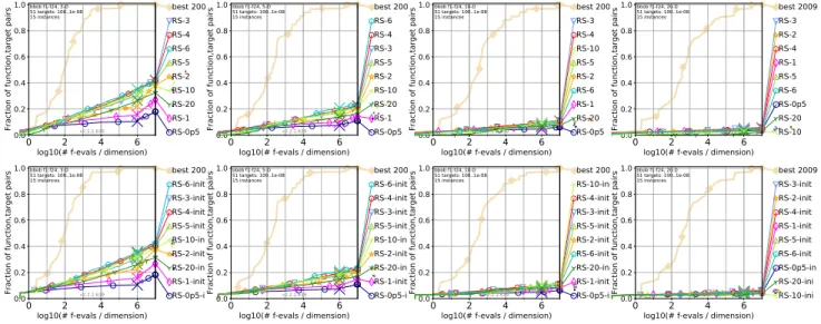
Global Performance Diﬀerences. In the aggregated empirical run-time distribution plots over all 24 bbob functions, some clear

tenden-cies can be observed. This is best seen for dimension 3 in Figure1

with the visible diﬀerences becoming smaller in higher dimension.2

Unsurprisingly, the results generally depend on the budget and the dimension. In 5-D, RS-3 solves in comparison the most problems

with a budget of 10 and 100× dimension, RS-4 with a budget of

1000 and 10,000× dimension and RS-6 for larger budgets. In 20-D,

RS-3 solves in comparison the most problems with a budget of

100× dimension, RS-4 with 1000 × dimension, and RS-6 with larger

budgets. These observations suggest that the easier target values are biased towards the center of the search space.

Note again here that the optima of the bbob functions are placed

uniformly at random in the hyperbox[−4,4]

n_{with the exception}

of the linear slope function for which the optimum lies at a corner

of the hyperbox[−5,5]nor even outside of it.

With increasing budget, only strategies with α ≥ 5 can be

op-timal, as only those are able to eventually solve all target values. However, log-linear extrapolation suggests a necessary evaluations

budget of roughly 10n×0.05p

to 10n×0.1p

evaluations to solve p percent of all problems which is even in moderate dimension far beyond any feasible number of evaluations to solve, say, 90% of all problems.

A too large sample volume decreases the performance for larger

budgets because outside of[−5,5]n, good targets can be hit only on

the linear function: RS-10 and RS-20 are clearly worse than RS-6. Interesting are the slopes of the empirical runtime distributions: with small sample volume, the slopes of the ECDFs decrease with larger budgets, whereas for sample volumes close to the

recom-mended “region of interest” of[−5,5]

n_{the slopes are roughly}

con-stant over the number of function evaluations.

Surprising in this context is the good performance of RS-6 that outperforms the other tested variants with smaller sample space

when the budget is high(er), i.e. for budgets larger than about 3⋅104×

dimension evaluations in dimension 5. The observable upsurge at 30 000×dimension evaluations in the empirical runtime distribution

1_{The actual wall clock times per function evaluation vary little with the diﬀerent}

variants and are, for ﬁxed dimension, mostly inﬂuenced by the other load on the machine: 8.6–9.6 microseconds (µs ) for dimension 2, 8.5–9.6 µs for dimension 3, 6.9–9.7 µs for dimension 5, 9.5–11 µs for dimension 10, 13–14 µs for dimension 20, and 23–24 µs for dimension 40.

2_{Most clear are the diﬀerences in dimension 2 (not shown here) with the same overall}

tendencies.

can be attributed to a great extend to the optimization of the linear

slope function (f5) that will be discussed below (see also Figures2

and3). A similar upsurge can be observed earlier for larger α . In

20-D however, the budget is too small to observe the upsurge at all. Evaluating the Search Space Origin. It has been noted that the

search space origin(0, . . . ,0) ∈ Rn is, by construction, an

espe-cially good search point, in particular for the Griewank Rosenbrock

function (f19). In order to not disfavor algorithms that do not

eval-uate this distinct solution in the beginning of the benchmarking, some example experiments of COCO evaluate the search space origin by default as the first search point. To compare the effect of this evaluation, we also re-run all random search variants with the origin evaluated before the uniform sampling starts. The corre-sponding algorithms are denoted with the suffix “-initIn0” in the

supplementary materialwhich, due to space limitations, we only

show selectively in this paper as in Figure1.

The main diﬀerence from evaluating the origin is observed on

the Griewank Rosenbrock function f19where evaluating the initial

search point(0, . . . ,0) reaches about 25% of the targets whereas

RS-0p5 reaches maximally about 16% of the targets in the ﬁrst evaluation and the percentage decreases with increasing α falling

below 10% for α≥ 3 (with slightly decreasing percentage in higher

dimensions), compare Figure6. When not evaluating the origin ﬁrst,

the random search needs some time to reach the same percentage of solved targets. Afterwards, both algorithms show again the same performance for larger budgets. In the larger dimensions, the experiments’ budget was not high enough for random search to reach 25% of the targets such that the period of similar performance cannot be observed.

In the following, we provide further observations on single func-tions that we ﬁnd remarkable and that let us understand some of the properties of the bbob functions.

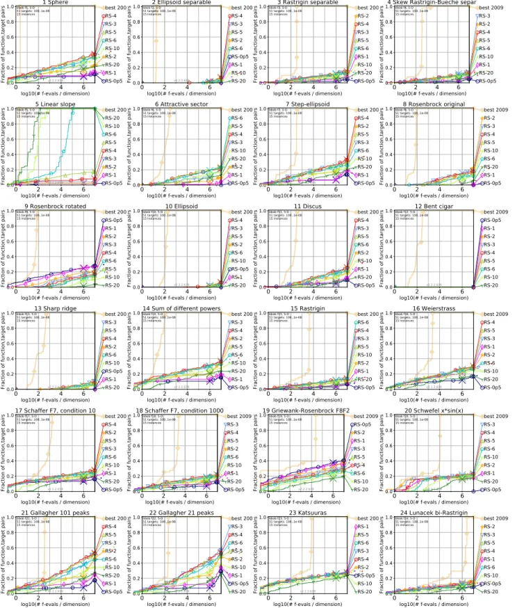
The linear slope function. The linear slope function (f5) is the

only bbob function that does not have its optimum in[−4,4]

n

but instead at one of the corners of the hypercube[−5,5]

n _and

beyond this corner where each variable is either≤ −5 or ≥ 5. This

explains why random search variants with sample volume larger

than[−5,5]

n_{perform best on this function.}

The linear function is the only one where in dimensions up to 10 all targets can be reached by some variants in the experiment budget. However, in 20-D, even the random search variant sampling

in[−20,20]

n_{cannot solve more than about 16% of all targets in}

106× dimension evaluations. For α → ∞, the probability to hit the

ﬁnal target approaches 2−n≈ 10−0.3n

, hence a budget of somewhat

above 100.3n

should suﬃce.

Katsuuras function. The Katsuuras function (f23) shows the largest

percentage of solved targets in higher dimension for all tested ran-dom search variants except for RS-10 and RS-20. Except for RS-10 and RS-20 all variants show comparable performance. This is

ex-pected as the function is repetitive within the hypercube[−α,α]

n

with α≤ 5.

Similar as on the Schaﬀer function f17, the ﬁrst evaluation in the

domain[−α,α]

n_{with α}_{≤ 5 solves comparably many targets like}

(4)

0 2 4 6 log10(# f-evals / dimension) 0.0 0.2 0.4 0.6 0.8 1.0

Fraction of function,target pairs _RS-0p5RS-1

RS-20 RS-10 RS-2 RS-5 RS-6 RS-4 RS-3 best 2009 bbob f1-f24, 3-D 51 targets: 100..1e-08 15 instances v2.2.2.639 0 2 4 6 log10(# f-evals / dimension) 0.0 0.2 0.4 0.6 0.8 1.0

Fraction of function,target pairs _RS-10RS-20

RS-0p5 RS-6 RS-5 RS-1 RS-4 RS-2 RS-3 best 2009 bbob f1-f24, 20-D 51 targets: 100..1e-08 15 instances v2.2.2.639 0 2 4 6 log10(# f-evals / dimension) 0.0 0.2 0.4 0.6 0.8 1.0

Fraction of function,target pairs _RS-0p5-inRS-1-init

RS-20-ini RS-2-init RS-10-ini RS-5-init RS-4-init RS-3-init RS-6-init best 2009 bbob f1-f24, 3-D 51 targets: 100..1e-08 15 instances v2.2.2.639 0 2 4 6 log10(# f-evals / dimension) 0.0 0.2 0.4 0.6 0.8 1.0

RS-20-ini RS-2-init RS-10-ini RS-5-init RS-3-init RS-4-init RS-6-init best 2009 bbob f1-f24, 5-D 51 targets: 100..1e-08 15 instances v2.2.2.639 0 2 4 6 log10(# f-evals / dimension) 0.0 0.2 0.4 0.6 0.8 1.0

RS-20-ini RS-6-init RS-2-init RS-5-init RS-3-init RS-4-init RS-10-ini best 2009 bbob f1-f24, 10-D 51 targets: 100..1e-08 15 instances v2.2.2.639 0 2 4 6 log10(# f-evals / dimension) 0.0 0.2 0.4 0.6 0.8 1.0

Fraction of function,target pairs _RS-10-iniRS-20-ini

RS-0p5-in RS-6-init RS-5-init RS-1-init RS-4-init RS-2-init RS-3-init best 2009 bbob f1-f24, 20-D 51 targets: 100..1e-08 15 instances v2.2.2.639

Figure 1: Empirical cumulative distribution functions of runtimes in dimensions 3, 5, 10, and 20 (from left to right) for

various random search variants, aggregated over all 24 bbob functions and 51 target precisions100. . .10

−8_{. The ﬁrst row shows}

the standard random search, sampling uniformly in[−α,α]

n _{with α indicated in the algorithm name RS-α while the second}

row shows the variants with the origin evaluated first. Compared to the algorithm variants that evaluate the search space origin first, we see another effect that is different from the Griewank Rosenbrock function, discussed above: for the func-tion value of the initial search point it does not make a difference

whether it is sampled within[−5,5]nor chosen as the origin. A

diﬀerence, however, occurs for the RS-10 and RS-20 variants (not shown here): in the case of RS-20, no other search point better than the origin is found in the entire experiment in 20-D and for RS-10,

it takes about 6 ⋅ 103function evaluations to ﬁnd a better target than

in the ﬁrst evaluation (also in 20-D). This eﬀect is smaller in lower and larger in higher dimension. In this sense, we can conclude that for the Katsuuras function, in contrast to the Griewank Rosenbrock function, the search space origin has no exceptionally good function

value compared to a random one within the hypercube[−5,5]

n

but that samples outside of this hypercube have exceptionally low function values.

The Gallagher functions. Besides the Griewank Rosenbrock and Katsuuras functions, the Gallagher functions show the best per-formance in low dimensions, solving all or almost all targets for variants RS-4, RS-5, and RS-6 in dimension 2 and showing the best performance over all functions (except for the linear slope) in dimension 5 with about 50% of the targets solved for RS-3 and RS-4. This good performance, however, is not observable in higher dimensions, where for example in 20-D, the performance on the Weierstrass function, the Schaﬀer function with condition number 10, the Griewank Rosenbrock, and the Katsuuras functions are better. Also the performance on the sphere function is slightly better in 20-D than for the Gallagher function with 21 peaks in the same dimension and for easier targets.

5 CONCLUSIONS

Despite being one of the simplest stochastic search variants, uni-form random search has an internal parameter, its sample volume, that plays an important role for its performance. We have com-pared different variants of random search on the bbob test suite and observed some significant differences on some functions that resulted in some insights into the construction of the function. Not surprisingly, only for the single bbob function that has its optimum

at one of the corners or outside the hypercube[−5,5]

n_{it is best to}

sample in a large volume. For some other functions such as the ro-tated Rosenbrock function and the Griewank Rosenbrock function, we observed that a smaller sample volume around the search space

origin is better for budgets up to 106× dimension.

Over all functions, the performance of RS-3, RS-4, RS-5, RS-6, and RS-10 is surprisingly similar, however also depending on the budget and dimension. The best performance is observed for the variants RS-4, RS-5, and in smaller dimension also RS-6 due to the

better performance on the linear function f5.

Evaluating the search space origin as ﬁrst solution has an ad-ditional advantage on several functions and in particular on the Griewank Rosenbrock function, where the origin has an exception-ally good function value by construction—an issue that has been

corrected in the recent bbob-largescale test suite [3].

The sample volume of RS-5 is in dimension 5, 10, and 20 about 3, 9, and 87 times larger than that of RS-4. That means, for example, with a 9 times larger budget, RS-5 will perform at least on par with RS-4 in dimension 10.

ACKNOWLEDGEMENTS

This work was supported by a public grant as part of the Investisse-ment d’avenir project, reference ANR-11-LABX-0056-LMH, LabEx

(5)

Fraction of function,target pairs RS-0p5

RS-1 RS-20 RS-2 RS-10 RS-6 RS-5 RS-3 RS-4 best 2009 bbob f1, 5-D 51 targets: 100..1e-08 15 instances v2.2.2.639 1 Sphere 0 2 4 6 log10(# f-evals / dimension) 0.0 0.2 0.4 0.6 0.8 1.0

Fraction of function,target pairs RS-20

RS-10 RS-1 RS-0p5 RS-6 RS-2 RS-5 RS-3 RS-4 best 2009 bbob f2, 5-D 51 targets: 100..1e-08 15 instances v2.2.2.639 2 Ellipsoid separable 0 2 4 6 log10(# f-evals / dimension) 0.0 0.2 0.4 0.6 0.8 1.0

RS-20 RS-10 RS-1 RS-6 RS-5 RS-3 RS-4 RS-2 best 2009 bbob f3, 5-D 51 targets: 100..1e-08 15 instances v2.2.2.639 3 Rastrigin separable 0 2 4 6 log10(# f-evals / dimension) 0.0 0.2 0.4 0.6 0.8 1.0

RS-20 RS-1 RS-10 RS-6 RS-5 RS-4 RS-2 RS-3 best 2009 bbob f4, 5-D 51 targets: 100..1e-08 15 instances v2.2.2.639

4 Skew Rastrigin-Bueche separ

RS-1 RS-2 RS-3 RS-4 RS-5 RS-6 RS-10 RS-20 best 2009 bbob f5, 5-D 51 targets: 100..1e-08 15 instances v2.2.2.639 5 Linear slope 0 2 4 6 log10(# f-evals / dimension) 0.0 0.2 0.4 0.6 0.8 1.0

RS-1 RS-2 RS-20 RS-10 RS-3 RS-4 RS-5 RS-6 best 2009 bbob f6, 5-D 51 targets: 100..1e-08 15 instances v2.2.2.639 6 Attractive sector 0 2 4 6 log10(# f-evals / dimension) 0.0 0.2 0.4 0.6 0.8 1.0

RS-1 RS-20 RS-10 RS-6 RS-3 RS-5 RS-2 RS-4 best 2009 bbob f7, 5-D 51 targets: 100..1e-08 15 instances v2.2.2.639 7 Step-ellipsoid 0 2 4 6 log10(# f-evals / dimension) 0.0 0.2 0.4 0.6 0.8 1.0

RS-1 RS-20 RS-6 RS-10 RS-5 RS-4 RS-3 RS-2 best 2009 bbob f8, 5-D 51 targets: 100..1e-08 15 instances v2.2.2.639 8 Rosenbrock original 0 2 4 6 log10(# f-evals / dimension) 0.0 0.2 0.4 0.6 0.8 1.0

RS-10 RS-5 RS-6 RS-4 RS-3 RS-2 RS-1 RS-0p5 best 2009 bbob f9, 5-D 51 targets: 100..1e-08 15 instances v2.2.2.639 9 Rosenbrock rotated 0 2 4 6 log10(# f-evals / dimension) 0.0 0.2 0.4 0.6 0.8 1.0

RS-1 RS-0p5 RS-10 RS-6 RS-2 RS-5 RS-3 RS-4 best 2009 bbob f10, 5-D 51 targets: 100..1e-08 15 instances v2.2.2.639 10 Ellipsoid 0 2 4 6 log10(# f-evals / dimension) 0.0 0.2 0.4 0.6 0.8 1.0

RS-20 RS-1 RS-10 RS-2 RS-6 RS-5 RS-3 RS-4 best 2009 bbob f11, 5-D 51 targets: 100..1e-08 15 instances v2.2.2.639 11 Discus 0 2 4 6 log10(# f-evals / dimension) 0.0 0.2 0.4 0.6 0.8 1.0

RS-10 RS-6 RS-5 RS-4 RS-3 RS-2 RS-1 RS-0p5 best 2009 bbob f12, 5-D 51 targets: 100..1e-08 15 instances v2.2.2.639 12 Bent cigar 0 2 4 6 log10(# f-evals / dimension) 0.0 0.2 0.4 0.6 0.8 1.0

RS-1 RS-0p5 RS-10 RS-6 RS-2 RS-4 RS-5 RS-3 best 2009 bbob f13, 5-D 51 targets: 100..1e-08 15 instances v2.2.2.639 13 Sharp ridge 0 2 4 6 log10(# f-evals / dimension) 0.0 0.2 0.4 0.6 0.8 1.0

RS-1 RS-20 RS-10 RS-6 RS-5 RS-2 RS-4 RS-3 best 2009 bbob f14, 5-D 51 targets: 100..1e-08 15 instances v2.2.2.639

14 Sum of different powers

RS-20 RS-1 RS-2 RS-10 RS-5 RS-3 RS-4 RS-6 best 2009 bbob f15, 5-D 51 targets: 100..1e-08 15 instances v2.2.2.639 15 Rastrigin 0 2 4 6 log10(# f-evals / dimension) 0.0 0.2 0.4 0.6 0.8 1.0

RS-20 RS-10 RS-6 RS-2 RS-1 RS-3 RS-5 RS-4 best 2009 bbob f16, 5-D 51 targets: 100..1e-08 15 instances v2.2.2.639 16 Weierstrass 0 2 4 6 log10(# f-evals / dimension) 0.0 0.2 0.4 0.6 0.8 1.0

RS-20 RS-1 RS-10 RS-6 RS-3 RS-5 RS-2 RS-4 best 2009 bbob f17, 5-D 51 targets: 100..1e-08 15 instances v2.2.2.639 17 Schaffer F7, condition 10 0 2 4 6 log10(# f-evals / dimension) 0.0 0.2 0.4 0.6 0.8 1.0

RS-20 RS-1 RS-10 RS-6 RS-2 RS-5 RS-4 RS-3 best 2009 bbob f18, 5-D 51 targets: 100..1e-08 15 instances v2.2.2.639 18 Schaffer F7, condition 1000 0 2 4 6 log10(# f-evals / dimension) 0.0 0.2 0.4 0.6 0.8 1.0

RS-10 RS-6 RS-4 RS-5 RS-3 RS-1 RS-2 RS-0p5 best 2009 bbob f19, 5-D 51 targets: 100..1e-08 15 instances v2.2.2.639 19 Griewank-Rosenbrock F8F2 0 2 4 6 log10(# f-evals / dimension) 0.0 0.2 0.4 0.6 0.8 1.0

RS-20 RS-1 RS-2 RS-10 RS-6 RS-5 RS-4 RS-3 best 2009 bbob f20, 5-D 51 targets: 100..1e-08 15 instances v2.2.2.639 20 Schwefel x*sin(x) 0 2 4 6 log10(# f-evals / dimension) 0.0 0.2 0.4 0.6 0.8 1.0

RS-1 RS-20 RS-10 RS-6 RS-2 RS-3 RS-5 RS-4 best 2009 bbob f21, 5-D 51 targets: 100..1e-08 15 instances v2.2.2.639 21 Gallagher 101 peaks 0 2 4 6 log10(# f-evals / dimension) 0.0 0.2 0.4 0.6 0.8 1.0

RS-0p5 RS-1 RS-10 RS-2 RS-5 RS-6 RS-4 RS-3 best 2009 bbob f22, 5-D 51 targets: 100..1e-08 15 instances v2.2.2.639 22 Gallagher 21 peaks 0 2 4 6 log10(# f-evals / dimension) 0.0 0.2 0.4 0.6 0.8 1.0

RS-10 RS-0p5 RS-2 RS-4 RS-3 RS-6 RS-5 RS-1 best 2009 bbob f23, 5-D 51 targets: 100..1e-08 15 instances v2.2.2.639 23 Katsuuras 0 2 4 6 log10(# f-evals / dimension) 0.0 0.2 0.4 0.6 0.8 1.0

RS-0p5 RS-10 RS-6 RS-1 RS-4 RS-5 RS-3 RS-2 best 2009 bbob f24, 5-D 51 targets: 100..1e-08 15 instances v2.2.2.639 24 Lunacek bi-Rastrigin

Figure 2: Empirical cumulative distribution of simulated (bootstrapped) runtimes, measured in number of objective function

evaluations, divided by dimension (FEvals/DIM) for the 51 targets 10[−8. .2]

(6)

RS-0p5 RS-1 RS-10 RS-2 RS-5 RS-3 RS-6 RS-4 best 2009 bbob f1, 10-D 51 targets: 100..1e-08 15 instances v2.2.2.639 1 Sphere 0 2 4 6 log10(# f-evals / dimension) 0.0 0.2 0.4 0.6 0.8 1.0

RS-10 RS-6 RS-5 RS-4 RS-3 RS-2 RS-1 RS-0p5 best 2009 bbob f2, 10-D 51 targets: 100..1e-08 15 instances v2.2.2.639 2 Ellipsoid separable 0 2 4 6 log10(# f-evals / dimension) 0.0 0.2 0.4 0.6 0.8 1.0

RS-10 RS-0p5 RS-1 RS-6 RS-5 RS-2 RS-4 RS-3 best 2009 bbob f3, 10-D 51 targets: 100..1e-08 15 instances v2.2.2.639 3 Rastrigin separable 0 2 4 6 log10(# f-evals / dimension) 0.0 0.2 0.4 0.6 0.8 1.0

RS-10 RS-0p5 RS-1 RS-6 RS-5 RS-2 RS-4 RS-3 best 2009 bbob f4, 10-D 51 targets: 100..1e-08 15 instances v2.2.2.639

4 Skew Rastrigin-Bueche separ

RS-1 RS-0p5 RS-3 RS-4 RS-5 RS-6 RS-10 RS-20 best 2009 bbob f5, 10-D 51 targets: 100..1e-08 15 instances v2.2.2.639 5 Linear slope 0 2 4 6 log10(# f-evals / dimension) 0.0 0.2 0.4 0.6 0.8 1.0

RS-0p5 RS-1 RS-10 RS-2 RS-6 RS-4 RS-3 RS-5 best 2009 bbob f6, 10-D 51 targets: 100..1e-08 15 instances v2.2.2.639 6 Attractive sector 0 2 4 6 log10(# f-evals / dimension) 0.0 0.2 0.4 0.6 0.8 1.0

RS-0p5 RS-10 RS-1 RS-6 RS-2 RS-5 RS-4 RS-3 best 2009 bbob f7, 10-D 51 targets: 100..1e-08 15 instances v2.2.2.639 7 Step-ellipsoid 0 2 4 6 log10(# f-evals / dimension) 0.0 0.2 0.4 0.6 0.8 1.0

RS-10 RS-6 RS-5 RS-1 RS-0p5 RS-4 RS-3 RS-2 best 2009 bbob f8, 10-D 51 targets: 100..1e-08 15 instances v2.2.2.639 8 Rosenbrock original 0 2 4 6 log10(# f-evals / dimension) 0.0 0.2 0.4 0.6 0.8 1.0

RS-10 RS-6 RS-5 RS-4 RS-3 RS-2 RS-1 RS-0p5 best 2009 bbob f9, 10-D 51 targets: 100..1e-08 15 instances v2.2.2.639 9 Rosenbrock rotated 0 2 4 6 log10(# f-evals / dimension) 0.0 0.2 0.4 0.6 0.8 1.0

RS-10 RS-6 RS-5 RS-4 RS-3 RS-2 RS-1 RS-0p5 best 2009 bbob f10, 10-D 51 targets: 100..1e-08 15 instances v2.2.2.639 10 Ellipsoid 0 2 4 6 log10(# f-evals / dimension) 0.0 0.2 0.4 0.6 0.8 1.0

RS-10 RS-0p5 RS-1 RS-6 RS-5 RS-2 RS-3 RS-4 best 2009 bbob f11, 10-D 51 targets: 100..1e-08 15 instances v2.2.2.639 11 Discus 0 2 4 6 log10(# f-evals / dimension) 0.0 0.2 0.4 0.6 0.8 1.0

RS-10 RS-6 RS-5 RS-4 RS-3 RS-2 RS-1 RS-0p5 best 2009 bbob f12, 10-D 51 targets: 100..1e-08 15 instances v2.2.2.639 12 Bent cigar 0 2 4 6 log10(# f-evals / dimension) 0.0 0.2 0.4 0.6 0.8 1.0

RS-10 RS-6 RS-5 RS-4 RS-3 RS-2 RS-1 RS-0p5 best 2009 bbob f13, 10-D 51 targets: 100..1e-08 15 instances v2.2.2.639 13 Sharp ridge 0 2 4 6 log10(# f-evals / dimension) 0.0 0.2 0.4 0.6 0.8 1.0

RS-0p5 RS-1 RS-10 RS-6 RS-2 RS-3 RS-5 RS-4 best 2009 bbob f14, 10-D 51 targets: 100..1e-08 15 instances v2.2.2.639

14 Sum of different powers

RS-0p5 RS-10 RS-1 RS-6 RS-2 RS-3 RS-5 RS-4 best 2009 bbob f15, 10-D 51 targets: 100..1e-08 15 instances v2.2.2.639 15 Rastrigin 0 2 4 6 log10(# f-evals / dimension) 0.0 0.2 0.4 0.6 0.8 1.0

RS-10 RS-0p5 RS-1 RS-6 RS-2 RS-4 RS-5 RS-3 best 2009 bbob f16, 10-D 51 targets: 100..1e-08 15 instances v2.2.2.639 16 Weierstrass 0 2 4 6 log10(# f-evals / dimension) 0.0 0.2 0.4 0.6 0.8 1.0

RS-10 RS-0p5 RS-1 RS-6 RS-2 RS-5 RS-3 RS-4 best 2009 bbob f17, 10-D 51 targets: 100..1e-08 15 instances v2.2.2.639 17 Schaffer F7, condition 10 0 2 4 6 log10(# f-evals / dimension) 0.0 0.2 0.4 0.6 0.8 1.0

RS-10 RS-0p5 RS-6 RS-1 RS-2 RS-3 RS-5 RS-4 best 2009 bbob f18, 10-D 51 targets: 100..1e-08 15 instances v2.2.2.639 18 Schaffer F7, condition 1000 0 2 4 6 log10(# f-evals / dimension) 0.0 0.2 0.4 0.6 0.8 1.0

RS-10 RS-6 RS-5 RS-4 RS-3 RS-2 RS-1 RS-0p5 best 2009 bbob f19, 10-D 51 targets: 100..1e-08 15 instances v2.2.2.639 19 Griewank-Rosenbrock F8F2 0 2 4 6 log10(# f-evals / dimension) 0.0 0.2 0.4 0.6 0.8 1.0

RS-0p5 RS-10 RS-6 RS-1 RS-5 RS-2 RS-4 RS-3 best 2009 bbob f20, 10-D 51 targets: 100..1e-08 15 instances v2.2.2.639 20 Schwefel x*sin(x) 0 2 4 6 log10(# f-evals / dimension) 0.0 0.2 0.4 0.6 0.8 1.0

RS-10 RS-6 RS-0p5 RS-3 RS-1 RS-4 RS-5 RS-2 best 2009 bbob f23, 10-D 51 targets: 100..1e-08 15 instances v2.2.2.639 23 Katsuuras 0 2 4 6 log10(# f-evals / dimension) 0.0 0.2 0.4 0.6 0.8 1.0

RS-10 RS-6 RS-5 RS-4 RS-0p5 RS-1 RS-3 RS-2 best 2009 bbob f24, 10-D 51 targets: 100..1e-08 15 instances v2.2.2.639 24 Lunacek bi-Rastrigin

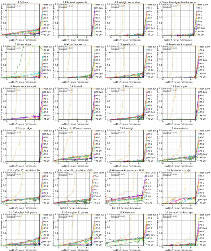
Figure 3: Empirical cumulative distribution of simulated (bootstrapped) runtimes, measured in number of objective function

evaluations, divided by dimension (FEvals/DIM) for the 51 targets 10[−8. .2]

(7)

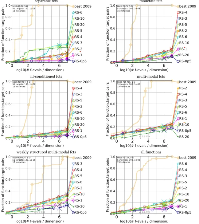
separable fcts moderate fcts

0 2 4 6

log10(# f-evals / dimension) 0.0 0.2 0.4 0.6 0.8 1.0

RS-2 RS-3 RS-4 RS-5 RS-20 RS-10 RS-6 best 2009 bbob f1-f5, 5-D 51 targets: 100..1e-08 15 instances v2.2.2.639 0 2 4 6

RS-1 RS-10 RS-6 RS-2 RS-5 RS-3 RS-4 best 2009 bbob f6-f9, 5-D 51 targets: 100..1e-08 15 instances v2.2.2.639 ill-conditioned fcts multi-modal fcts 0 2 4 6

Fraction of function,target pairs _RS-20RS-0p5

RS-10 RS-1 RS-6 RS-5 RS-3 RS-4 RS-2 best 2009 bbob f15-f19, 5-D 51 targets: 100..1e-08 15 instances v2.2.2.639

weakly structured multi-modal fcts all functions

0 2 4 6

RS-20 RS-10 RS-2 RS-5 RS-3 RS-4 RS-6 best 2009 bbob f1-f24, 5-D 51 targets: 100..1e-08 15 instances v2.2.2.639

Figure 4: Bootstrapped empirical cumulative distribution of the number of objective function evaluations divided by

dimen-sion (FEvals/DIM) for 51 targets with target precidimen-sion in 10[−8. .2]

for all functions and subgroups in 5-D. As reference algorithm, the best algorithm from BBOB 2009 is shown as light thick line with diamond markers.

(8)

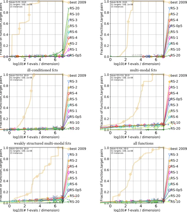
separable fcts moderate fcts

0 2 4 6

RS-6 RS-1 RS-5 RS-0p5 RS-4 RS-2 RS-3 best 2009 bbob f6-f9, 20-D 51 targets: 100..1e-08 15 instances v2.2.2.639 ill-conditioned fcts multi-modal fcts 0 2 4 6

RS-0p5 RS-1 RS-6 RS-5 RS-4 RS-2 RS-3 best 2009 bbob f10-f14, 20-D 51 targets: 100..1e-08 15 instances v2.2.2.639 0 2 4 6

RS-6 RS-5 RS-3 RS-0p5 RS-4 RS-1 RS-2 best 2009 bbob f15-f19, 20-D 51 targets: 100..1e-08 15 instances v2.2.2.639

weakly structured multi-modal fcts all functions

0 2 4 6

RS-0p5 RS-6 RS-5 RS-1 RS-4 RS-2 RS-3 best 2009 bbob f20-f24, 20-D 51 targets: 100..1e-08 15 instances v2.2.2.639 0 2 4 6

RS-0p5 RS-6 RS-5 RS-1 RS-4 RS-2 RS-3 best 2009 bbob f1-f24, 20-D 51 targets: 100..1e-08 15 instances v2.2.2.639

Figure 5: Bootstrapped empirical cumulative distribution of the number of objective function evaluations divided by

di-mension (FEvals/DIM) for 51 targets with target precision in 10[−8. .2]

for all functions and subgroups in 20-D. As reference algorithm, the best algorithm from BBOB 2009 is shown as light thick line with diamond markers.

(9)

0 2 4 6

RS-10 RS-6 RS-0p5 RS-5 RS-4 RS-3 RS-2 RS-1 best 2009 bbob f19, 3-D 51 targets: 100..1e-08 15 instances v2.2.2.639 19 Griewank-Rosenbrock F8F2 0 2 4 6

Fraction of function,target pairs RS-20-ini

RS-10-ini RS-5-init RS-0p5-in RS-4-init RS-6-init RS-3-init RS-2-init RS-1-init best 2009 bbob f19, 3-D 51 targets: 100..1e-08 15 instances v2.2.2.639 19 Griewank-Rosenbrock F8F2 0 2 4 6

RS-10 RS-6 RS-5 RS-4 RS-3 RS-2 RS-1 RS-0p5 best 2009 bbob f19, 10-D 51 targets: 100..1e-08 15 instances v2.2.2.639 19 Griewank-Rosenbrock F8F2 0 2 4 6

Fraction of function,target pairs RS-20-ini

RS-10-ini RS-6-init RS-5-init RS-4-init RS-3-init RS-2-init RS-1-init RS-0p5-in best 2009 bbob f19, 10-D 51 targets: 100..1e-08 15 instances v2.2.2.639 19 Griewank-Rosenbrock F8F2

Figure 6: Empirical cumulative distribution functions of the runtime to reach certain targets on the Griewank-Rosenbrock function for the random search variants without (ﬁrst and third plot) and with evaluating the origin ﬁrst (second and forth) in dimension (left two plots) and dimension 10 (right two plots).

LMH, in a joint call with Gaspard Monge Program for optimization, operations research and their interactions with data sciences.

REFERENCES

[1] Anne Auger, Dimo Brockhoﬀ, Nikolaus Hansen, Dejan Tuˇsar, Tea Tuˇsar, and To-bias Wagner. 2016. The impact of search volume on the performance of RANDOM-SEARCH on the bi-objective BBOB-2016 test suite. In Genetic and Evolutionary Computation Conference Companion Proceedings (GECCO 2016). ACM, 1257–1264. [2] Anne Auger and Raymond Ros. 2009. Benchmarking the pure random search

on the BBOB-2009 testbed. In GECCO (Companion), Franz Rothlauf (Ed.). ACM, 2479–2484.

[3] Ouassim Elhara, Konstantinos Varelas, Duc Nguyen, Tea Tusar, Dimo Brock-hoﬀ, Nikolaus Hansen, and Anne Auger. 2019. COCO: The Large Scale Black-Box Optimization Benchmarking (bbob-largescale) Test Suite. arXiv preprint arXiv:1903.06396 (2019).

[4] S. Finck, N. Hansen, R. Ros, and A. Auger. 2009. Real-Parameter Black-Box Opti-mization Benchmarking 2009: Presentation of the Noiseless Functions. Technical

Report 2009/20. Research Center PPE. http://coco.lri.fr/downloads/download15.

03/bbobdocfunctions.pdfUpdated February 2010.

[5] N. Hansen, A Auger, D. Brockhoﬀ, D. Tuˇsar, and T. Tuˇsar. 2016. COCO:

Perfor-mance Assessment. ArXiv e-printsarXiv:1605.03560(2016).

[6] N. Hansen, A. Auger, O. Mersmann, T. Tuˇsar, and D. Brockhoﬀ. 2016. COCO: A Platform for Comparing Continuous Optimizers in a Black-Box Setting. ArXiv

e-printsarXiv:1603.08785(2016).

[7] N. Hansen, S. Finck, R. Ros, and A. Auger. 2009. Real-Parameter Black-Box Opti-mization Benchmarking 2009: Noiseless Functions Deﬁnitions. Technical Report

RR-6829. INRIA. http://coco.lri.fr/downloads/download15.03/bbobdocfunctions.pdf

Updated February 2010.

[8] N. Hansen, T. Tuˇsar, O. Mersmann, A. Auger, and D. Brockhoﬀ. 2016. COCO: The

Experimental Procedure. ArXiv e-printsarXiv:1603.08776(2016).

[9] Tea Tuˇsar, Dimo Brockhoﬀ, Nikolaus Hansen, and Anne Auger. 2016. COCO: the bi-objective black box optimization benchmarking (BBOB-BIOBJ) test suite. ArXiv