HAL Id: hal-02996319
https://hal.uca.fr/hal-02996319
Submitted on 9 Nov 2020
HAL is a multi-disciplinary open access
archive for the deposit and dissemination of sci-entific research documents, whether they are pub-lished or not. The documents may come from teaching and research institutions in France or abroad, or from public or private research centers.
L’archive ouverte pluridisciplinaire HAL, est destinée au dépôt et à la diffusion de documents scientifiques de niveau recherche, publiés ou non, émanant des établissements d’enseignement et de recherche français ou étrangers, des laboratoires publics ou privés.
To cite this version:
Loïs Martinek, Nathalie Bolfan-Casanova. Water quantification in olivine and wadsleyite by Raman 2spectroscopy and study of errors and uncertainties. American Mineralogist, Mineralogical Society of America, 2020, �10.2138/am-2021-7264�. �hal-02996319�
Revision 3
1Water quantification in olivine and wadsleyite by Raman
2spectroscopy and study of errors and uncertainties
3MARTINEK LOÏS1AND BOLFAN-CASANOVA NATHALIE1
4
1Laboratoire Magmas et Volcans, 6 avenue Blaise Pascal, TSA 60026 – CS 60026, 63178 Aubière Cedex
5
A
BSTRACT6
The study of nominally anhydrous minerals with vibrational spectroscopy, despite its 7
sensitivity, tends to produce large uncertainties (in absorbance or intensity) if the observed 8
dispersion of the values arising from the anisotropy of interaction with light in non-cubic 9
minerals is not assessed. In this study, we focused on Raman spectroscopy, which allows the 10
measurement of crystals down to few micrometers in size in back-scattered geometry, and with 11
any water content, down to 200 ppm by weight of water. Using synthetic hydrous single-crystals 12
of olivine and wadsleyite, we demonstrate that under ideal conditions of measurement and 13
sampling, the data dispersion reaches ±30% of the average (at 1σ) for olivine, and ±32% for 14
wadsleyite, mostly because of their natural anisotropy. As this anisotropy is linked to physical 15
properties of the mineral, it should not be completely considered as error without treatment. By 16
simulating a large number of measurements with a 3D model of the OH/Si spectral intensity ratio 17
for olivine and wadsleyite as a function of orientation, we observe that although dispersion 18
increases when increasing the number of measured points in the sample, analytical error 19
points (five to ten, depending on the measurement method), the greatest contribution to the error 21
on the measured intensities is related to the instrument’s biases, and reaches 12 to 15% in ideal 22
cases, indicating that laser and power drift corrections have to be carefully performed. We finally 23
applied this knowledge on error sources (to translate data dispersion into analytical error) on 24
olivine and wadsleyite standards with known water contents to build calibration lines for each 25
mineral in order to convert the intensity ratio of the water bands over the structural bands (OH/Si) 26
to water content. The conversion factor from OH/Si to ppm by weight of water (H2O) is
27
93108±24005 for olivine, 250868±45591 for bearing wadsleyite, and 57546±13916 for iron-28
free wadsleyite, showing the strong effect of iron on the spectral intensities. 29
Keywords: wadsleyite, olivine, nominally anhydrous minerals, Raman spectroscopy,
30
water quantification 31
I
NTRODUCTION32
Even though the major mineral phases of the Earth's mantle are nominally anhydrous, 33
many of them are known to contain water as OH point defects in their structure (Bell and 34
Rossman, 1992; Smyth and Keppler, 2006; Peslier 2010; Demouchy & Bolfan-Casanova, 2016). 35
The water storage capacity of the most abundant upper mantle mineral, namely olivine, has been 36
the subject of many studies, however most reports concern simple systems or single crystal 37
olivine (e.g. Kohlstedt et al. 1996; Withers & Hirschmann 2007 and 2008; Bali et al. 2008; 38
Kovács et al. 2010; Férot & Bolfan-Casanova 2012; Litasov et al. 2014, Yang et al. 2016). 39
Single-phase experiments allow the growth of single crystals large enough to be suitable for any 40
analytical method, especially absorption infrared spectroscopy using Fourier transform infrared 41
(FTIR), secondary ion mass spectrometry (SIMS), or elastic recoil detection analysis (ERDA). 42
In experiments with natural mantle compositions on the other hand, olivine, 43
orthopyroxene, clinopyroxene and garnet can coexist, strongly limiting crystal growth. These 44
samples often display crystal sizes from 20 to 50 µm, limiting the use of the conventional 45
methods cited above on the fine-grained samples. Investigation of the storage capacity in more 46
complex systems such as peridotite has been carried out and the small grain size of the grains 47
required the use of SIMS (few tens of cubic micrometers analyzed) or even nano-SIMS (one or 48
two order of magnitude less) ( see Ardia et al., 2012; Tenner et al., 2012; Novella et al., 2014). 49
This technique is complicated to use because of high background levels of H, complex 50
preparation to avoid H contamination and the need for well-characterized standards (Koga et al. 51
2003, Mosenfelder et al. 2011). 52
FTIR is frequently used sensitive technique to quantify hydroxyl content in nominally 53
anhydrous minerals, which also gives structural information about H point defects. Reliable 54
methods exist to quantify water in anisotropic minerals using FTIR, and a consequent literature 55
exists on the subject (e.g., Libowitzsky and Rossman 1996; Asimow et al. 2006; Kovács et al. 56
2008; Withers et al. 2012, Withers 2013; Qiu et al. 2018). However, in the case of very water-57
rich samples as, for example, wadsleyite, a high-pressure polymorph of olivine, that can contain 58
up to 3.2 weight percent of water (Inoue et al., 1995), infrared spectroscopy requires an important 59
thinning of the samples (which may cause their loss) in order to avoid the entire absorption of the 60
infrared signal. 61
In this study, we used confocal polarized Raman spectroscopy (the laser source being 62
polarized, the incident beam is therefore also polarized). This technique offers several advantages 63
for water quantification in synthetic minerals with a small grain size and low to very high water 64
spectroscopy requires only one side of the sample to be polished, while double polishing is 66
required in the measurement of absorbance using FTIR. Unfortunately, very thin polishing of the 67
sample can irremediably damage them, especially those sintered under conditions where fluids 68
are highly wetting, which is the case of the conditions of the deep upper mantle (Yoshino et al. 69
2007). The detection limit of water quantification using Raman spectroscopy (around 70
50-100 ppm wt) may be a problem with samples synthesized under conditions of the uppermost 71
mantle, where the water solubility is the lowest for many mineral species (Férot & Bolfan-72
Casanova 2012, Yang 2016), but any higher concentration can be measured (Bolfan-Casanova et 73
al. 2014). The spot size of confocal Raman spectroscopy (3-5 µm) allows measurements on very 74
fine-grained samples (down to crystal sizes around 5 µm) without difficulties. The time required 75
for reasonably precise measurements (some minutes) is low enough to multiply the number of 76
measured points on different crystals throughout the sample and have a statistically correct 77
coverage of the whole sample. One major drawback of Raman spectroscopy is that the intensity 78
absorption depends on many factors in addition to the concentration, such as the intensity of the 79
incident laser, confocality and lens magnification, which control the volume of sample that is 80
excited by the laser beam. Moreover, the chosen gratings and the optics of the spectrometer 81
(instrument-dependent parameters), as well as the optical properties of the sample or its surface 82
state will affect the efficiency of the measurement (see e.g. Mercier et al. 2009, Schiavi et al. 83
2018; Zarei et al. 2018). In contrast, the absorbance measured using FTIR depends solely on the 84
thickness, concentration and absorptivity of the sample itself, following a relationship known as 85
the Beer-Lambert law. In addition, in absorbance spectroscopy the intensity transmitted by the 86
sample is always normalized to that of the incident beam, which tends to eliminate instrumental 87
biases on the intensity of the signal from the sample. 88
Raman spectroscopy is widely used to quantify H2O concentrations in glasses or melt
89
inclusions (e.g., Thomas et al. 2008; Mercier et al. 2009; Schiavi et al., 2018). In these studies, 90
quantification of the water concentration relies on the comparison of the OH/Si of the unknown 91
to that of well-characterized standards measured under identical conditions, as the OH intensity 92
has been shown to increase linearly with water content. Here, OH/Si is defined by the integrated 93
intensity of the water band normalized to that of the silicate vibrations (see the following section 94
for details). As numerous factors may affect the measurement efficiency (such as variation of 95
focusing depth or surface quality), using the ratio of the OH band area over that of silica bands 96
area reduces the data dispersion or scatter, as both regions are equally affected by focusing or 97
surface variations. Calibrations of the method have been proposed by Thomas et al. (2008 and 98
2015) for garnet, Bolfan-Casanova et al. (2014) for olivine, Thomas et al. (2015) for ringwoodite, 99
and Weis et al. (2018) for orthopyroxene (this last study having used also forward-scattering). 100
Previous water content quantification in olivine conducted with Raman spectroscopy 101
often display large error bars on their results (Bolfan-Casanova et al. 2014). In this study, we 102
demonstrate that those error bars are significantly related to the dispersion (used in the statistical 103
meaning of the term throughout this work) of the relative intensities of the different vibrational 104
modes caused by the anisotropy of the minerals. As this anisotropy is a natural consequence of 105
the structure and symmetry of the crystal, it is not directly related to error, and can even be used 106
to get information on orientation (see for example Ishibashi et al. 2008). Firstly, we studied the 107
relative effect of the different error sources and of anisotropy on the statistical dispersion of 108
measurements in hydrated olivine and wadsleyite single crystals and used it to propose a method 109
to estimate the analytical error from the data dispersion of the measurements using polarized 110
unanalyzed Raman spectroscopy. We then propose a calibration for water quantification in 111
olivine and wadsleyite based on standards characterized by FTIR or ERDA methods. 112
M
ETHODS113
Synthesis of olivine and wadsleyite 114
Olivine and wadsleyite single crystals were synthesized in the multi-anvil press at 12 and 115
15 GPa and at 1200 and 1350 °C from San Carlos olivine as starting material. Olivine single 116
crystals and powder were placed in a folded rhenium foil capsule, placed itself in a welded gold-117
palladium capsule containing brucite powder. The experimental assembly consisted of an MgO 118
octahedron containing Cr2O3, a zirconia thermal insulator, a LaCrO3 heater with molybdenum
119
electrodes in contact with the anvils and an MgO central part containing the capsule. Temperature 120
was controlled using a W-Re thermocouple (5% and 26% Re). Experiments were conducted at 121
the Laboratoire Magmas et Volcans (LMV, Clermont-Ferrand, France) on a Voggenreiter Mavo-122
press LP 1500 tons multi-anvil press equipped with a Kawai-Endo apparatus. Heating was 123
performed and controlled by a Pacific 140-AMX AC power source. Secondary anvils were 32 124
mm tungsten carbide cubes with 8 and 6 mm truncations. Olivine synthesis duration was 4.5 125
hours at 1200 °C, and wadsleyite synthesis lasted 2 hours at 1350 °C. For both syntheses, 126
temperature was gradually decreased after the experiment (around 50 °C per minute) instead of 127
quenching to prevent crystal fracturation. Recovered crystals were oriented using polarized light 128
microscopy for olivine and X-ray diffraction for wadsleyite, and then cut and mirror polished 129
perpendicular to crystallographic axes (see Figure 1). Olivine and wadsleyite are both 130
orthorhombic so display an anisotropic behavior with respect to light absorption. Wadsleyite has 131
been reported to become monoclinic above 0.5 wt % H2O using X-ray diffraction (Jacobsen et al.
2005), however we did not detect any noticeable spectral difference that could be due to this 133
small change in the β-angle. 134
FTIR spectroscopy 135
Most of the samples used in order to calibrate the Raman quantification method were 136
olivines characterized using FTIR by Férot & Bolfan-Casanova (2012). These water content 137
values were updated using the most recent calibration of the infrared extinction coefficient (ε) 138
determined using ERDA by Withers et al. (2012) of 45200 l molH2O-1 cm-2 instead of the 28450 l
139
molH2O-1 cm-2 value given by Bell et al. (2003). This decreases all the water contents of olivine
140
reported in Férot and Bolfan-Casanova (2012) by a factor of 1.589. 141
Polarized spectra acquired for this study were collected on a Vertex70 Brucker 142
spectrometer coupled to a Hyperion microscope with a 15× lens, condenser and knife-edge 143
apertures creating a rectangular target area of 40-50 µm. Samples were analyzed on a CaF2 plate
144
at a resolution of 2 cm-1, with 200 to 300 accumulations. After background subtraction and
145
atmospheric correction, a cubic baseline correction has been applied on the 1500 to 4000 cm-1
146
area, and integration calculated in the 2700 to 3720 cm-1 area. The absorbance is then used to
147
calculate the H2O content based on Beer Lambert's law (see equation 1) with the integrated molar
148
absorption coefficient (also called extinction coefficient) cited above, and a density factor X of 149
5521 l·molH2O-1 (used to convert molH2O·l-1 to ppm by weight of H2O, equal to 18.02×10⁶/ρ). The
150
density ρ has been calculated from Fischer & Medaris (1969) accounting for the olivine 151
composition. The equation used is the following, with ε being the infrared extinction coefficient, 152
Atot the total absorbance, and d the thickness of the sample in centimeters:
Equation 1 154 𝐶𝐻2𝑂 = 𝑋 × 𝐴𝑡𝑜𝑡 𝜀 × 𝑑 Raman spectroscopy 155
Raman spectra were collected at LMV using an InVia confocal Raman micro-156
spectrometer manufactured by Renishaw and equipped with a 532 nm diode laser (200 mW 157
output power), a Peltier-cooled CCD detector of 1024×256 pixels, a motorized XYZ stage and a 158
Leica DM 2500M optical microscope. Scattered light was collected in a back-scattered geometry. 159
An edge filter effectively reduced both Rayleigh scattered photons and photons from the exciting 160
laser source at 0 cm-1 that had been reflected by the sample surface. A 2400 grooves/mm grating
161
was used for the analyses, which resulted in a spectral resolution between 1.3 cm-1 (around 100 162
cm-1) and 0.72 cm-1 (around 3700 cm-1). All spectra were acquired with polarized light without
163
analyzer, and sample was rotated under the beam to change the polarization angle. A ×100 164
microscope lens (numerical aperture 0.9) was used and the slit aperture was set to 20 μm (high 165
confocality setting). Daily calibration of the spectrometer was performed based on a Si 520.5 166
cm−1 peak. The effective laser power (changed by filters) used was 65 to 71 mW for olivine, and 167
8 to 9 mW for wadsleyite and glass (low enough power to prevent destabilization and 168
dehydration) and was measured to normalize spectra to 1 mW. A power of 125 to 140 mW can 169
cause some damages on water-rich olivine, and a power of 15 mW caused a slight OH intensity 170
reduction in wadsleyite with very high water content (sample 2054, 3.4% in weight), but no 171
dehydration or destabilization effect has been observed with the lower laser power values finally 172
chosen. A hydrous basaltic glass (see Schiavi et al. 2018) is used to check and be able to correct 173
for power drifts and efficiency drifts along the different area of measurement. 174
As already stated above, the quantification of water concentration is based on the 175
measurement of the OH band integrated intensity normalized to the silicate band integrated 176
intensity. Under static conditions of measurement, the window analyzed using a grating of 2400 177
groves/mm decreases from approximately 1200 cm-1 at low wavenumbers to 800 cm-1 at high
178
wavenumbers. For all samples and standards, Si area refers to wavenumbers from 61 to 1318 179
cm-1 centered on 720 cm-1, and OH area refers to wavenumbers from 2978 to 3784 cm-1 centered
180
on 3400 cm-1. Both areas were chosen to contain all the needed peaks and bands. Acquisition
181
times are short for the Si area because of its high intensity, to prevent saturation of the CCD 182
detector, and longer for the OH area to increase the signal to noise ratio, the OH bands being 183
much weaker. Thus, acquisition times were 2×5 s for the Si area, and 5×60 s for the OH area of 184
olivine and wadsleyite. For the glass, the acquisition times were 4×10 s for the Si area, and 185
5×120 s for the OH area. The daily variations of the spectrometer were corrected by normalizing 186
to the average OH/Si intensity ratio of the hydrated glass measured in each measurement session, 187
each of those consisting on two random points on the glass sample, providing a more 188
reproducible OH/Si intensity ratio here called (OH/Si)Smp_Norm. The normalization operation is
189
shown in equation 2, where (OH/Si)Smp Meas is the average OH/Si of the measured sample,
190
(OH/Si)Glass_Meas is the standard glass OH/Si measured in the same session as the sample, and
191
(OH/Si)Glass_Std is the measurement of the OH/Si of the glass measured in the same session as the
192
standards. The result is the normalized OH/Si of the sample (OH/Si)Smp_Norm.
193 Equation 2 194 OH Si𝑆𝑚𝑝 𝑁𝑜𝑟𝑚 =OH Si𝑆𝑚𝑝 𝑀𝑒𝑎𝑠 × OH Si𝐺𝑙𝑎𝑠𝑠 𝑆𝑡𝑑 OH Si𝐺𝑙𝑎𝑠𝑠 𝑀𝑒𝑎𝑠
The procedure of baseline correction is essential in obtaining reproducible values of 195
OH/Si for each phase (see Figure 2 and supplementary materials 1). The baseline shape is linear 196
for the olivine Si area (rarely cubic), cubic for its OH area, cubic or polygonal for the wadsleyite 197
Si area and cubic for its OH area. The anchor points used to define the baseline are shown in 198
Figure 2. The spectra used afterwards for integrations are the raw spectra subtracted of the 199
baseline, and divided by the total acquisition time and the laser power, to normalize each 200
spectrum to a power of 1 mW and an acquisition time of 1 s. It has to be noted that this is not the 201
unit of the spectra, as the intensity measured on each spectrum depends on various parameters of 202
the instrument such as the grating and the wave number, but can be labelled as counts·s-1·mW-1.
203
Integration consists in the area under the curve of the baseline-corrected and normalized 204
spectrum: [200, 1100] for the Si area and [3050, 3700] for the OH area of olivine, and [300, 205
1100] for the Si area and [3150, 3700] for the OH area of wadsleyite (see Figure 2). The result of 206
this integration defines thereafter the intensity of the spectra. In the case of wadsleyite, iron-207
bearing samples display a very intense band at 171 cm-1 that merges with the white line (at low
208
wavenumbers) rendering its baseline correction unreliable due to the difficult anchoring of the 209
baseline at low wavenumbers (see supplementary materials 1). This is why the integration of the 210
Si area of wadsleyite starts at a higher wavenumber of 300 cm-1.
211
For all the spectra of glass, the single-crystal spectra and some of the wadsleyite and 212
olivine samples, one measurement point consists in the OH intensity divided by the Si intensity 213
(OH/Si ratio) with the same polarization angle, and is referred as "single points". On most of the 214
olivine and wadsleyite samples, one measurement point will be the average of two OH/Si ratio 215
obtained from two measurements on the same crystal with orthogonal polarization angles, and is 216
referred as "orthogonal couples". 217
The averaged OH/Si values of several measurement points on a sample is the value used 218
to compare the different samples. Eight olivine and seven wadsleyite standard samples of various 219
known water contents have been used to build the calibration lines allowing the conversion from 220
OH/Si ratio to water content. Water contents of olivine standards have been determined by FTIR, 221
using Withers et al. (2012) extinction coefficient, and those of wadsleyite standards were 222
measured by ERDA (Bolfan-Casanova et al. 2018). 223
R
ESULTS224
Quantification of the OH/Si variation related to mineral orientation 225
In order to assess the effect of orientation alone on the dispersion of the average OH/Si 226
value of each phase, polarized Raman spectra have been acquired on each face of the prepared 227
single crystals of olivine and wadsleyite. We acquired 19 spectra, from 0 to 180°, on each face 228
for both OH and Si area, and values for 190 to 350° were calculated by symmetry. Normalized 229
OH/Si values were then fitted using equation 3 for olivine and equation 4 for wadsleyite (see 230 Figure 3). 231 Equation 3 232 OH Si (𝜃) = 𝐻 + 𝑎1 × cos 2(𝜃 + 𝑑 1) Equation 4 233 OH Si (𝜃) = 𝐻 + 𝑎1× cos 2(𝜃 + 𝑑 1) + 𝑎2× cos2(2 ∗ (𝜃 + 𝑑2))
Here, H is a constant depicting the minimum value for a given face adjusting the vertical 234
position of the curve; a1 is the amplitude (the difference between the maximum and minimum
intensities of the given face for equation 3) of the cosine describing the features with a period of 236
180° (2-fold symmetry) shifted of an angle d1; a2 is the amplitude of the cosine describing the
237
features with a period of 90° (4-fold symmetry) shifted of an angle d2. Each parameter has been
238
optimized to minimize the differences between the measurement data and the fitted curve. It has 239
to be noted that the necessity for introducing parameters d arise from the fact that crystals are not 240
exactly polished following the crystallographic axes. These fits are thus empirical and only serve 241
the purpose of creating a model of the analyzed crystals. For olivine, this misalignment is around 242
10° (as visible in Figure 3), and has later been neglected (the maxima of the faces (100) and (010) 243
have been aligned along crystallographic axes in the 3D model). On the other hand, the 244
misalignment of wadsleyite is high, and orientation has been lost, rendering necessary the use of 245
the shift parameters d. The observed component with a 90° period is necessary in the case of 246
wadsleyite to fit correctly the measured intensity, and can mostly be noticed in the fits of the 247
intensity variations on the faces arbitrarily called F1, F2 and F3 (see M F1 and M F2 fit curves 248
around 150 and 330°). 249
Considering that the single-crystal analyzed is homogeneous in water content, the only 250
source of deviation between the modeled curve and the measured data is the combination of data 251
treatment error and measurement error. Data treatment error has been estimated from the 252
differences between repeated baseline correction and treatments of Raman spectra, and will be 253
referred as ETr in following equations, tables and figures. The estimated values for ETr on OH/Si
254
are 3.6% for olivine and 4.0% for wadsleyite. This error tends to remain small when the signal to 255
noise ratio is high enough. The second error source taken into account is the one caused by all 256
measurement uncertainties, such as surface irregularities or focus offset, and will be referred as 257
EMeas. Supposing that EMeas and ETr are independent sources of error, the deviation of
measurement points from the model is the square root of the sum of the two error sources 259
squared, and is provided by the fit shown in Figure 3. From this calculation, we obtain a 260
measurement related uncertainty EMeas reaching 4.4% for olivine, and 4.1% for wadsleyite. The
261
last source of error arises from the daily variation of the spectrometer efficiency and the method 262
used to correct it. Hence, the treatment and measurement errors related to this correction are the 263
cause of an additional error of 11.9%, and will be referred as ECor. This value has been estimated
264
accounting for the measurement and data treatment errors related to the standard glass 265
measurement. The first two error, EMeas and ETr, sources apply on each point separately, while the
266
correction error ECor applies to all the points of a measurement session. The values of the
267
estimated errors are reported in table 1. 268
The intensity versus angle model curves (as shown in Figure 3) were then used to build a 269
3D model of OH/Si variation as a function of crystallographic orientation. In Figure 3 it is visible 270
that the fitted curves do not coincide with the corresponding minima and maxima from the other 271
faces (for example, the maxima of the “a” and “b” curves for olivine are different, but both 272
describe the OH/Si intensity parallel to the “c” axis and should be equal). These differences are 273
very likely to be caused by misalignment of the polished faces with respect to the 274
crystallographic axes. To obtain a continuous set of three curves in 3D (as depicted by the bold 275
lines in Figure 4), the amplitudes of the curves have been increased or decreased so that they 276
cross each other along the crystallographic axes, keeping at the same time the average value of 277
each curve constant. Intermediate orientation values were completed by combining those 278
acquired along crystallographic axes, each point of any orientation being obtained with equation 279
5: 280
Equation 5 281 (𝑂𝐻 𝑆𝑖 )𝛼 = ∑ ( 𝑂𝐻 𝑆𝑖 )𝑖× cos 2(𝛼 𝑖)
In this equation, any orientation α is defined by a vector with a norm equal to the 282
corresponding (OH/Si)α value. This vector has one projection on each of the “a”, “b” and “c”
283
planes corresponding to values (OH/Si)i fitted with equation 3 or 4 for a given angle (see Figure
284
3). (OH/Si)α is then calculated as being the sum of these three (OH/Si)i, each multiplied by the
285
squared cosine of the angle between the defined vector and its projection on the corresponding 286
plane. This operation results in a peanut-shaped three-dimensional OH/Si model for each phase 287
when displayed in a 3D polar graph (see Figure 4, depicting OH/Si variation in olivine and 288
supplementary materials 2 for wadsleyite). The OH/Si is depicted here as the distance between 289
the peanut-shaped surface and the intersection of the a, b, and c axes. In both olivine and 290
wadsleyite cases, it can be observed that high OH/Si values are located along one axis, identified 291
as the c-axis for olivine, and that variations seem approximately axisymmetric for both of them. 292
This modelling process can be applied to other orthorhombic minerals (or quadratic), each model 293
being based on its own measured OH/Si values (as shown in Figure 3). Minerals with other 294
crystal system could still be modelled, but they might require a different procedure of polishing, 295
measurement and 3D model extrapolation. 296
Distinguishing OH/Si natural dispersion and errors 297
The 3D OH/Si distribution models for olivine and wadsleyite have then been used as basis 298
to simulate measurements, in order to untangle the effects of natural dispersion (i.e. due to 299
crystallographic orientation) and analytical uncertainties on the final error for any type of 300
measurement (single points or orthogonal couples) and as a function of the number of 301
measurement points. To achieve this, the first step is to generate a set of random uniformly 302
distributed crystal orientations that simulates a polycrystalline sample. A random “longitude” 303
angle between 0 and 360° is first generated (uniform distribution), and a second “latitude” angle 304
is generated with a semicircle distribution with a maximal probability for 0° and a probability of 305
reaching zero when approaching 90 or -90°. To each orientation corresponds an OH/Si value 306
determined as described for the construction of the 3D model. On each point chosen among those 307
of this surface, the estimated measurement and treatment errors are applied, using equation 6. 308
Here, XMeas and XTr represent normally distributed random values with an average of zero, and a
309
standard deviation equal to the desired error component EMeas or ETr. Each “modeled”, or
310
simulated point (OH/Si)M has its own XMeas and XTr values, because those errors do apply on
311
every point separately and independently, finally yielding the "real" value (OH/Si)R.
312 Equation 6 313 OH Si𝑅 = OH Si𝑀 × (1 + 𝑋𝑀𝑒𝑎𝑠) × (1 + 𝑋𝑇𝑟)
For single point measurements, the simulated sample value will be the average of all the 314
(OH/Si)R, multiplied in the same way by 1 + XCor to simulate the errors arising from the laser
315
power drift correction. In the case of orthogonal couples measurements, the two resulting 316
(OH/Si)R values of each measurement point are averaged, then all points are again averaged
317
before applying the 1 + XCor factor.
318
All the error and dispersion values used in the following section are expressed as relative 319
errors, in percent of deviation from the average. Hereafter, the goal is to get the standard 320
deviation and the average of each simulated measurement session for any number of 321
statistically significant as possible. In this study, final values have been obtained for sets of 2 to 323
30 points in both single point and orthogonal couples, with one million draws for each case. For 324
each number of points, the average of all the standard deviations of all sets of values has been 325
interpreted as the expected measured dispersion DTh, and the standard deviation of all the
326
averages of all the set of points has been interpreted as the error expected for the measurement 327
(ETh). Both DTh and ETh depend on the number of measurement points and on the technique used
328
for the measurement (single point or orthogonal couples). Dispersion increases when adding 329
points, reaching an approximate plateau past 10 points, and error decreases when adding points, 330
but stabilizes much slower past 30 points, limited by the contribution of ECor to the final error
331
(see Figure 5). 332
The dispersion and error values obtained by the above simulation were then fitted to 333
obtain error propagation equations as a function of the number of points, the measurement 334
method, and the different errors sources. The natural dispersion caused by anisotropy can be 335
estimated from equation 7 below. Here DNat is the natural dispersion, which is the expected
336
relative standard deviation obtained on a random set of measurements without any kind of error 337
added as a function of the number of points (N). DAn represents the total anisotropy, and is the
338
same standard deviation as DNat, but for an infinite set of points, and finally "a" is a fitting
339
parameter (all the values of the different parameters are shown in Table 1). 340
Equation 7
341
𝐷𝑁𝑎𝑡 = 𝐷𝐴𝑛− 𝑎 𝑁 − 1
Equations 8 and 9 also express the dispersion of values and in addition takes into account 342
the errors arising from measurement and data treatment. As the normalization related errors (ECor)
apply on all the points in the same way, it does not have any effect on the relative dispersion. 344
Equation 8 gives the expected dispersion for single points measurements, and equation 9 for 345
orthogonal couples. Here, DAn, "a" and N are the same as in equation 7, EMeas is the measurement
346
error, and ETr is the data treatment error.
347 Equation 8 348 𝐷𝑇ℎ = √𝐷𝐴𝑛2 + 𝐸𝑀𝑒𝑎𝑠2 + 𝐸𝑇𝑟2 − 𝑎 𝑁 − 1 Equation 9 349 𝐷𝑇ℎ = √𝐷𝐴𝑛2 +𝐸𝑀𝑒𝑎𝑠 2 + 𝐸 𝑇𝑟2 2 − 𝑎 𝑁 − 1
The theoretical uncertainties follow a simple error propagation equation, which is 350
expressed as shown in equation 10 for single points measurements, and equation 11 for 351
orthogonal couples. Here, ECor plays a role on the final relative error and tends to account for
352
most of the uncertainty when the number of points increases (see Figure 5). 353 Equation 10 354 𝐸𝑇ℎ = √𝐷𝐴𝑛 2 + 𝐸 𝑀𝑒𝑎𝑠2 + 𝐸𝑇𝑟2 𝑁 + 𝐸𝐶𝑜𝑟 2 Equation 11 355 𝐸𝑇ℎ = √𝐷𝐴𝑛2 + 𝐸𝑀𝑒𝑎𝑠2 + 𝐸 𝑇𝑟2 2 𝑁 + 𝐸𝐶𝑜𝑟 2
Each of the above equations can be applied for both olivine and wadsleyite. All the 356
parameters are displayed in Table 1. 357
It can be noted that all the dispersions and errors in this simulation neglect the initial 358
asymmetry of the distribution of the OH/Si values (see distribution histograms in supplementary 359
materials 3 and 4) which, although abnormal and strongly asymmetric (towards high values for 360
single points measurements and low values for the orthogonal couples), rapidly tends toward a 361
Gaussian-shaped distribution above 10 to 15 points. Moreover, the asymmetry of the distribution 362
might be very difficult to observe on a real set of measurement because of the limited set of 363
points in which the distribution of values may not have any statistical significance. Hence, the 364
deviation caused by this hypothesis tends to be negligible above 10 to 15 measurement points, 365
but very low number of points should still follow a very asymmetric distribution, increasing 366
error. 367
It can be noted that the measurement and treatment errors have a very small effect on both 368
the dispersion and the error (see Figure 5). On the other hand, power drift correction related 369
errors (ECor) have a very strong effect on the final error, demonstrating that this step must be
370
carefully performed in order to get correct values. An important result is that the use of averaged 371
orthogonally polarized measurements roughly halves the theoretical dispersion of the values, thus 372
decreasing the associated error. The total expected dispersion directly related to anisotropy 373
(neglecting all the other error sources) for olivine is around ±29.4% for single points and ±14.8% 374
for orthogonal couples. Wadsleyite displays slightly higher values, with 32.5% and 16.8% (all 375
these values are shown in Table 1). The same effect could be reached on single points 376
measurements with approximately four times more points. Another advantage of using the 377
orthogonal couples is that it forces to measure more diverse grain orientations in the sample, 378
hence limiting the effect of a potential preferential crystallographic orientation within the sample. 379
To sum up, assuming a chemically homogeneous sample (in terms of water content), if 380
the standard deviation is close to the expected dispersion (calculated with equations 8 or 9), the 381
real analytical error is given by equations 10 or 11. It follows that, in the ideal case of randomly 382
oriented crystals, the error on OH/Si for 5 to 10 measurement points is between 15 and 18% for 383
single points, and 12 and 15% for orthogonal couples. A deviation inferior to the expected 384
deviation (still assuming that the sample is homogeneous) would point out an insufficient 385
sampling of the natural dispersion. A rough estimation of the real error in this case can be 386
obtained with equation 12. Here, the difference between the expected deviation DTh and the
387
measured value DSmp causes the final error (ESmp) to increase from the ideal value ETh to the total
388
dispersion DTh, equal to the error expected on a measurement based on one single measurement
389
point. 390
In contrast, if the standard deviation is higher than DTh, whether because the sample is
391
heterogeneous or the measurements are too defective, the error "reduction" from DSmp to ESmp
392
(from equations 8 or 9 to equations 10 or 11) may not be reasonable to apply directly. 393
Considering that the sampling is sufficient in this case, an error approximation can be obtained 394
from equation 10 (variables are the same as in equation 13). 395 Equation 12 396 𝐸𝑆𝑚𝑝 = 𝐷𝑇ℎ− (𝐷𝑇ℎ− 𝐸𝑇ℎ) × 𝐷𝑆𝑚𝑝 𝐷𝑇ℎ
Equation 13 397 𝐸𝑆𝑚𝑝 = √(𝐷𝑆𝑚𝑝× 𝐸𝑇ℎ 𝐷𝑇ℎ ) 2 + (𝐷𝑆𝑚𝑝− 𝐷𝑇ℎ) 2
Olivine and wadsleyite calibration lines 398
The water content of the samples used to build the calibration lines are shown in Table 2, 399
along with the values of OH/Si measured with Raman spectroscopy. The calibration lines (see 400
equation 14 and Figure 6) are built with least-square minimization, always pass by the origin, and 401
take into account the effect of the water content uncertainties arising from FTIR and ERDA 402
measurements as well as the Raman measurement. All the error bars on the OH/Si have been 403
estimated with the method described above. Some samples thus display a relatively large error 404
bar (such as 949 or M380b, see Figure 6 and Table 2) because the measured dispersion was 405
significantly greater than the expected dispersion (obtained from equations 8 to 11). On the other 406
hand, some samples, such as M382, displayed a very low dispersion that may be related to 407
insufficient sampling, once again resulting in a larger error bar. The factor to convert from OH/Si 408
to ppm in weight of water (F in equation 11) is 93108±24005 for olivine, 250868±45591 for 409
wadsleyite (with iron), and 57546±13916 for wadsleyite (without iron). This result shows the 410
tremendous effect of iron on the spectrum's shape and intensity, implying that chemical 411
composition has to be verified in order to quantify the water content of wadsleyite. There are two 412
identified causes to this difference, the first being that for two samples with comparable water 413
contents, the Si area of an iron-free wadsleyite displays sharper peaks, even if their heights are 414
comparable, implying a lower Si intensity. However, at the same time, its OH area is more 415
intense. This causes the OH/Si of an iron-free wadsleyite to be much higher than the one of an 416
iron-bearing wadsleyite with a comparable water content (see supplementary materials 5). Figure 417
6 displays the calibration lines for olivine and wadsleyite. 418
Equation 14
419
C𝐻2𝑂(𝑝𝑝𝑚 𝑤𝑡) = 𝐹 × OH
Si𝑆𝑚𝑝 𝑁𝑜𝑟𝑚
The uncertainty on the slope obtained for each calibration has to be added to the final 420
error ESmp described above, the total uncertainty on the water content being given by equation 15,
421
where EH2O is the total error, ESmp is the total relative error on the OH/Si of the sample, and ECal is
422
the calibration-related relative error. The same can be applied to dispersions. 423
424
Equation 15
425
𝐸𝐻2𝑂 = √𝐸𝑆𝑚𝑝2 + 𝐸𝐶𝑎𝑙2
The uncertainty on the slope of the calibration line (as shown in Figure 6) arising from the 426
errors in water quantification of the standards and from the error on their OH/Si often becomes 427
the major component of the total uncertainty on the water content compared to the error on the 428
measurement of OH/Si with Raman spectroscopy. 429
Regarding olivine, the 26% uncertainty on the calibration line is much larger than the 430
12% error on the OH/Si measurement attained for a large number of points (in the case of 431
orthogonal couples, see Figure 5). Following equation 15, this 12% error (ESmp) increases to 29%
432
only because of the uncertainty on the calibration (ECal). The same problem applies to wadsleyite
433
with the 18% error on the calibration line for bearing wadsleyite and the 24% error for iron-434
free wadsleyite. The greater is the error on the OH/Si of the sample (because of insufficient 435
sampling or sample heterogeneities), the smaller the contribution of calibration uncertainties to 436
the total error will be (see Figure 7). 437
D
ISCUSSION438
The quantification of as much error and uncertainty sources as possible provides a better 439
understanding of the data dispersion inherent to the use of Raman spectroscopy on anisotropic 440
crystals. The relative impact of each source of error highlights what affects the more the final 441
error, showing where further progress and developments could be made. The first issue is the 442
laser-drift during and between different sessions. The method used to overcome this problem 443
brings an additional source of error (referred as ECor throughout this study), as it implies two
444
OH/Si ratio measurements on a standard glass, thus adding twice data treatment and 445
measurement error to the result (divided by √2, as the value measured is supposed to be the same 446
for the two measurements). Moreover, as this correction has to be applied on all the points of a 447
sample, its contribution to the total error does not decrease with an increasing number of points. 448
Consequently, its relative contribution increases, and becomes the major part of the error on the 449
OH/Si ratio above around 20 to 25 single points, or 5 orthogonal couples (see Figure 5). This 450
power-drift correction error is also responsible for a significant part of the calibration error, thus 451
acting in two different ways in the final error. On the other hand, insufficient sampling of the 452
natural dispersion rapidly causes the final error to be larger than the measured dispersion (see 453
equation 11). Orthogonally polarized averaged measurements, improving by force the sampling 454
of various orientations (and thus, anisotropy) help to prevent from orientation biases. 455
Secondly, the effect of the calibration uncertainty (caused by the errors on each standard 456
point) on the final error acts similarly as the power-drift correction uncertainty (both are 457
insensitive to the number of points), rapidly becoming the major part of the error, particularly for 458
olivine. Focusing on the ideal case where the dispersion observed on the sample (DSmp) equals the
459
theoretical dispersion (DTh), implying that ESmp and ETh are equal, the conversion factors DH2O/
460
EH2O (following equation 15, and applying this to the dispersion by replacing ESmp with DSmp to
461
obtain DH2O) and DSmp/ESmp of wadsleyite are superior to those of olivine in all cases (except for
462
two points in the orthogonal couples case, see Figure 7). This is caused by the higher effect of the 463
error sources on DTh than on ETh in the case of wadsleyite, where ECor mitigates their effect, hence
464
increasing DSmp/ESmp. Adding ECal does not change this observation, except that it mitigates these
465
effects, lowering the expected "gain" on errors, with higher attenuation for higher ECal (see Figure
466
7). In the case of a poor sampling, accounting for ECal tends to mitigate the effect of the error
467
augmentation (see equation 9) by increasing ESmp to a much higher EH2O, lowering the effect of
468
equation 15. 469
Water content heterogeneities may cause the measured dispersion to be larger than the 470
expected one. In such cases, when the ratio of observed over expected dispersion is close to one, 471
even if the gain may seem high, it is important to consider that chemical heterogeneities should 472
remain as low as possible (see the discussion around equation 13). The present water 473
quantification method by Raman spectroscopy relies on the hypothesis that only the orientation 474
varies from one crystal to another, and that these orientations are distributed randomly and 475
uniformly. This means that chemically heterogeneous samples (should it be a major element 476
content variation, or in water content variation) are unsuitable for precise water quantification 477
with this method. In the case of wadsleyite, we observed that the iron content has a tremendous 478
effect on the calibration line slope, implying that composition has to be measured to verify if all 479
the analyzed crystals have a similar iron content. The problem of the random distribution of 480
orientations in samples also has to be considered, as preferential orientation may occur in some 481
samples. However, if a sample is chemically homogeneous, a sample with a strong disparity of 482
orientations could be identified if it displays values dispersion much smaller than the expected 483
dispersion (see discussion around equation 12). 484
C
ONCLUSION485
Raman spectroscopy allows the water content measurement of samples of any size above 486
few micrometers, and with water contents down to 150-200 ppm in weight (see Bolfan-Casanova 487
et al. 2014), with no observed upper limit, where many other methods may require large samples, 488
or are unsuitable for very high water contents (FTIR). Even if vibrational spectroscopy is very 489
useful to discriminate OH point defects over contamination, the sensitivity to crystallographic 490
orientation in anisotropic samples often leads to high standard deviations in the measurements of 491
water content (Férot and Bolfan-Casanova 2012). Here we show that a large part of this 492
dispersion may be related to the natural anisotropy of the measured mineral, and is thus normal. 493
The main objective of this work was to be able to calculate the error associated to the 494
measurement of water content in olivine and wadsleyite, using Raman spectroscopy, knowing the 495
anisotropy of the OH/Si ratio for each phase. We identified throughout this study various sources 496
of error. The major parameters (beside anisotropy) affecting errors on the final values are the 497
uncertainties on the calibration line, insufficient sampling of anisotropy, and the laser-drift 498
correction errors. Nevertheless, most of the errors obtained with this procedure fall in a range of 499
20-25% of relative error for wadsleyite, and 25-30% for olivine, making Raman spectroscopy 500
still suitable for quantification water content in olivine and wadsleyite. The detailed study of the 501
error sources has provided a greater understanding of the method, and has allowed an 502
improvement of the treatment methods, reducing significantly the uncertainties arising from this 503
part of the procedure. 504
I
MPLICATIONS505
The high spatial resolution of Raman spectroscopy allows the study of water distribution 506
among different phases of fine polymineralic samples of complex (natural) composition, with a 507
wide range of measurable water contents. Although relatively high, the uncertainties on water 508
concentration are sufficiently low to infer the effect of thermodynamic intensive parameters on 509
water incorporation. The method proposed here can also be applied to all orthorhombic minerals. 510
A
CKNOWLEDGMENTS511
The authors thank Jean-Louis Fruquière and Cyrille Guillot for their help and advises on 512
the experimental assemblies, István Kovács, Anthony Withers, and Mainak Mookherjee for very 513
precise and helpful reviews of this manuscript, Federica Schiavi and Arnaud Guillin for fruitful 514
discussions, and Laurent Jouffret for the time spent on the orientation attempt of the wadsleyite 515
single crystal with X-ray diffraction. The multi-anvil apparatus of Laboratoire Magmas et 516
Volcans is financially supported by the CNRS (Instrument national de l’INSU). This is 517
Laboratory of Excellence ClerVolc contribution N° 419. 518
R
EFERENCES519
Ardia, P., Hirschmann, M.M., Withers, A.C., and Tenner, T.J. (2012) H2O storage capacity of 520
olivine at 5–8 GPa and consequences for dehydration partial melting of the upper mantle. 521
Earth and Planetary Science Letters, 345-348, 104-116. 522
Asimow, P.D., Stein, L.C., Mosenfelder, J.L., and Rossman, G.R. (2006) Quantitative polarized 523
infrared analysis of trace OH in populations of randomly oriented mineral grains. 524
American Mineralogist, 91, 278-284. 525
Bali, E., Bolfan-Casanova, N., and Koga, K.T. (2008) Pressure and temperature dependence of H 526
solubility in forsterite: An implication to water activity in the Earth interior. Earth and 527
Planetary Science Letters, 268, 354-363. 528
Bell, D.R., and Rossman, G.R. (1992) Water in Earth's mantle: The role of nominally anhydrous 529
minerals. Science, 255, 1391-1397. 530
Bell, D.R., Rossman, G.R., Maldener, J., Endisch, D., and Rauch, F. (2003) Hydroxide in olivine: 531
A quantitative determination of the absolute amount and calibration of the IR spectrum. 532
Journal of Geophysical Research, 108, 2105. 533
Bolfan-Casanova, N., Montagnac G. and Reynard B. (2014) Measurements of water contents in 534
olivine using Raman spectroscopy. American Mineralogist 99, 149-156. 535
Bolfan-Casanova N., Schiavi, F., Novella, D., Bureau, H., Raepsaet, C., Khodja, H., and 536
Demouchy S. (2018) Examination of Water Quantification and Incorporation in 537
Transition Zone Minerals Wadsleyite, Ringwoodite and Phase D Using ERDA (Elastic 538
Recoil Detection Analysis). Frontiers in Earth Science, 6, 75. 539
Demouchy, S., and Bolfan-Casanova, N. (2016) Distribution and transport of hydrogen in the 540
lithospheric mantle: A review. Lithos, 240-243, 402-425. 541
Férot, A., and Bolfan-Casanova, N. (2012) Water storage capacity in olivine and pyroxene to 14 542
GPa: Implications for thewater content of the Earth’s upper mantle and nature of seismic 543
discontinuities. Earth and Planetary Science Letters, 349-350, 218-230. 544
Fischer, G.W., and Medaris, L.G. (1969) Cell dimensions and X-ray determinative curve for 545
synthetic Mg-Fe olivines. American Mineralogist, 54, 741-753. 546
Inoue, T., Yurimoto, H., and Kudoh, Y. (1995) Hydrous modified spinel, Mg1.75SiH0.5O4: A 547
new water reservoir in the mantle transition region. Geophysical Resaerch Letters, 22, 548
issue 2, 117-120. 549
Ishibashi, H., Arakawa, M., Ohi, S., Yamamoto, J., Miyake, A., and Kagi, H. (2008) Relationship 550
between Raman spectral pattern and crystallographic orientation of a rock-forming 551
mineral: a case study of Fo89Fa11 olivine. Journal of Raman Spectroscopy, 39, 1653-552
1659. 553
Jacobsen, S.D, Demouchy, S., Frost, D.J., Boffa Ballaran, T., and King, J. (2005) A systematic 554
study of OH in hydrous wadsleyite from polarized FTIR spectroscopy and single-crystal 555
X-ray diffraction: Oxygen sites for hydrogen storage in Earth's interior. American 556
Mineralogist, 90, 61-70. 557
Koga, K., Hauri, E., Hirschmann, M.M., and Bell, D. (2003) Hydrogen concentration analyses 558
using SIMS and FTIR: Comparison and calibration for nominally anhydrous minerals. 559
Geochemistry Geophysics Geosystems, 4, number 2, 1019. 560
Kohlstedt, D.L., Keppler, H., and Rubie, D.C. (1996) Solubility of water in the α, β and γ phases 561
of (Mg,Fe)2SiO4. Contributions to Mineralogy and Petrology, 123, 345-357. 562
Kovács, I., Hermann, J., O'Neill, H.S.C., Fitz Gerald, J., Sambridge, M., and Horváth, G. (2008) 563
Quantitative absorbance spectroscopy with unpolarized light: Part II. Experimental 564
evaluation and development of a protocol for quantitative analysis of mineral IR spectra. 565
American Mineralogist, 93, 765-778. 566
Kovács, I., O'Neill, H.S.C., Hermann, J. and Hauri, E.H. (2010) Site-specific infrared O-H 567
absorption coefficients for water substitution into olivine. American Mineralogist 95, 292-568
299. 569
Libowitzky, E., and Rossman, G.R. (1996) Principles of quantitative absorbance measurements in 570
anisotropic crystals. Physics and Chemistry of Minerals, 23, 319-327. 571
Litasov, K.D., Shatskiy, A., and Ohtani, E. (2014) Melting and subsolidus phase relations in 572
peridotite and eclogite systems with reduced C–O–H fluid at 3–16GPa. Earth and 573
Planetary Science Letters, 391, 87-99. 574
Mercier, M., Di Muro, A., Giordano, D., Métrich, N., Lesne, P., Pichavant, M., Scaillet, B., 575
Clocchiatti, R., Montagnac, G. (2009) Influence of glass polymerisation and oxidation on 576
micro-Raman water analysis in alumino-silicate glasses. Geochimica et Cosmochimica 577
Acta, 73, 197-217. 578
Mosenfelder, J.L., Le Voyer, M., Rossman, G.R., Guan, Y., Bell, D.R., Asimow, P.D., and Eiler, 579
J.M. (2011) Analysis of hydrogen in olivine by SIMS: Evaluation of standards and 580
protocol. American Mineralogist, 96, 1725-1741. 581
Novella, D., Frost, D.J., Hauri, E.H., Bureau, H., Raepsaet, C., and Roberge, M. (2014) The 582
distribution of H2O between silicate melt and nominally anhydrous peridotite and the 583
onset of hydrous melting in the deep upper mantle. Earth and Planetary Science Letters, 584
400, 1-13. 585
Peslier, A.H. (2010) A review of water contents of nominally anhydrous natural minerals in the 586
mantles of Earth, Mars and the Moon. Journal of Volcanology and Geothermal Research, 587
197, 239-258. 588
Qiu, Y., Jiang, H., Kovács, I., Xia, Q.K. and Yang, X. (2018) Quantitative analysis of H-species 589
in anisotropic minerals by unpolarized infrared spectroscopy: An experimental evaluation. 590
American Mineralogist, 103, 1761-1769. 591
Schiavi, F., Bolfan-Casanova, N., Withers, A.C., Médard, E., Laumonier, M., Laporte, D., 592
Flaherty, T., and Gómez-Ulla, A. (2018) Water quantification in silicate glasses by 593
Raman spectroscopy: Correcting for the effects of confocality, density and ferric iron. 594
Chemical Geology, 483, 312-331. 595
Smyth, J.S., and Keppler, H., Eds. (2006) Water in nominally anhydrous minerals. Reviews in 596
Mineralogy and Geochemistry, 62. 597
Tenner, T.J., Hirschmann, M.M., Withers, A.C., and Ardia, P. (2012) H2O storage capacity of 598
olivine and low-Ca pyroxene from 10 to 13 GPa: consequences for dehydration melting 599
above the transition zone. Contributions to Mineral Petrology, 163, 297-316. 600
Thomas, S.M., Thomas, R., Davidson, P., Reichart, P., Koch-Müller, M., and Dollinger, G. 601
(2008) Application of Raman spectroscopy to quantify trace water concentrations in 602
glasses and garnets. American Mineralogist, 93, 1550-1557. 603
Thomas, S.M., Jacobsen, S.D., Bina, C.R., Reichart, P., Moser, M., Hauri, E.H., Koch-Müller, 604
M., Smyth, J.R., and Dollinger, G. (2015) Quantification of water in hydrous ringwoodite. 605
Frontiers in Earth Sciences, 2, 38. 606
Thomas, S.M., Wilson, K., Koch-Müller, M., Hauri, E.H., McCammon, C., Jacobsen, S.D., 607
Lazarz, J., Rhede, D., Ren, M., Blair, N., and Lenz, S. (2015) Quantification of water in 608
majoritic garnet. American Mineralogist, 100, 1084-1092. 609
Weis, F.A., Lazor, P., and Skogby, H. (2018) Hydrogen analysis in nominally anhydrous 610
minerals by transmission Raman spectroscopy. Physics and Chemistry of Minerals, 45, 611
597-607. 612
Withers, A.C., and Hirschmann, M.M. (2007) H2O storage capacity of MgSiO3 clinoenstatite at 613
8-13 GPa, 1100-1400°C. Contributions to Mineralogy and Petrology, 154, 663-674. 614
Withers, A.C., and Hirschmann, M.M. (2008) Influence of temperature, composition, silica 615
activity and oxygen fugacity on the H2O storage capacity of olivine at 8 GPa. 616
Contributions to Mineralogy and Petrology, 156, 595-605. 617
Withers, A.C., Bureau, H., Raepsaet, C., and Hirschmann, M.M. (2012) Calibration of infrared 618
spectroscopy by elastic recoil detection analysis of H in synthetic olivine. Chemical 619
Geology, 334, 92-98. 620
Withers, A.C. (2013) On the use of unpolarized infrared spectroscopy for quantitative analysis of 621
absorbing species in birefringent crystals. American Mineralogist, 98,689–697 622
Yang, X. (2016) Effect of oxygen fugacity on OH dissolution in olivine under peridotite-623
saturated conditions: An experimental study at 1.5-7 GPa and 1100-1300°C. Geochimica 624
et Cosmochimica Acta, 173, 319-336. 625
Yoshino, T., Nishihara, Y., Karato, S. ichiro (2007) Complete wetting of olivine grain boundaries 626
by a hydrous melt near the mantle transition zone. Earth and Planetary Science Letters, 627
256, 466-472 628
Zarei, A., Klumbach, S., and Keppler, H. (2016) The relative Raman scattering cross sections of 629
H2O and D2O, with implications for in situ studies of isotope fractionation. ACS Earth
630
and Space Chemistry, 2, 925-934. 631
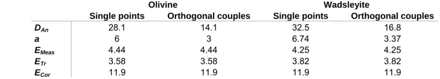
Table 1: Fitting parameters (DAn and a) and estimated error sources values (E) for
633
dispersion and error equations (equations 6 to 13). DAn is the calculated anisotropy contribution to
634
the observed values deviation; EMeas is the measurement related error, ETr the treatment related
635
error, and ECor the laser-drift correction related error.
636
Olivine Wadsleyite
Single points Orthogonal couples Single points Orthogonal couples
DAn 28.1 14.1 32.5 16.8 a 6 3 6.74 3.37 EMeas 4.44 4.44 4.25 4.25 ETr 3.58 3.58 3.82 3.82 ECor 11.9 11.9 11.9 11.9 637
Table 2: Standards used for the olivine and wadsleyite calibrations of OH/Si versus H2O
638
concentration in ppm by weight of water. Wadsleyite* standards are iron-free. Raman 639
measurement type "1" refers to the case of single point measurement and "2" to the case of 640
orthogonal couples. 641
Source measurement Raman measurement Sample Phase Method ppm wt H2O error Type Points OH/Si error
949 Olivine FTIR 1304 290 1 8 0.01534 0.00371 M497 Olivine ERDA 750 38 1 10 0.00405 0.00081 M589 Olivine FTIR 1244 596 1 57 0.01127 0.00141 1033 Olivine FTIR 522 176 2 11 0.00806 0.00118 895b Olivine FTIR 180 21 2 12 0.00382 0.00156 1044b Olivine FTIR 1766 674 2 10 0.01924 0.00250 M817 Olivine FTIR 640 215 2 10 0.00350 0.00103 M818 Olivine FTIR 291 72 2 10 0.00269 0.00104 M230 Wadsleyite ERDA 1045 52 1 10 0.01591 0.00270
M226A Wadsleyite ERDA 4209 210 2 12 0.03863 0.00642 M380b Wadsleyite ERDA 12206 610 1 10 0.04219 0.01833 M382 Wadsleyite ERDA 27271 1364 2 13 0.10122 0.01864 M226B Wadsleyite* ERDA 4000 200 2 10 0.10574 0.01457 2053 Wadsleyite* ERDA 21600 1080 1 10 0.46945 0.10382 2054 Wadsleyite* ERDA 34000 1700 1 10 0.49357 0.07957 642
F
IGURE CAPTIONS643
Figure 1 : Optical image of the olivine and wadsleyite samples used for the anisotropy 644
quantification. 645
646
Figure 2 : Raman spectra of olivine (grey) and wadsleyite (black) in the silicate region 647
and the OH region. The wide bars underneath each graph (light bar for olivine, dark bar for 648
wadsleyite) depict the integration window used for water quantification. The darker short lines 649
depict the anchor point area used for baseline correction. The baseline shape is linear for olivine 650
Si area, and cubic for OH area, and is polylinear for wadsleyite Si area, and cubic for OH area. 651
652
Figure 3 : OH/Si values of olivine (top) and wadsleyite (bottom) as a function of the 653
orientation of the crystal relative to the beam, for three perpendicular faces. Error bars are the 654
estimated uncertainties linked to measurement errors and data treatment (see text). Horizontal 655
error bars are an estimation of the angle's error. Solid and dashed lines (M) represent the fitted 656
curves obtained through equation 3 (or 4 for wadsleyite). Olivine crystallographic faces were 657
identified, whereas for wadsleyite, faces are named arbitrarily (F1, F2 and F3). 658
659
Figure 4 : Three-dimensional plot of OH/Si values of olivine (as fitted in Figure 3) as a 660
function of crystallographic orientation. Values obtained with incident beam parallel to the a axis 661
are displayed in the (100) (bc) plane, and so on for the other faces. Grey points (which due to 662
their density may be displayed as light grey lines here) are the extrapolations of the solid lines 663
(derived from Figure 3) for any given orientation (see equation 5). 664
665
Figure 5 : Simulated relative dispersions (empty circles) and errors (solid circles) for 666
olivine (top) and wadsleyite (bottom), for the case of single point measurements (left) and 667
orthogonal couples (right), expressed in percent deviation from the average. Light grey symbols 668
stand for the contribution of anisotropy (An) alone. Adding the measurement (Meas) uncertainties 669
yields the intermediate grey symbols (mostly hidden by the dark grey ones). Adding treatment 670
(Tr) uncertainties gives the dark grey symbols, and finally adding the uncertainty arising from the 671
power correction (Cor) yields the black circles. 672
673
Figure 6 : Calibration lines for olivine (top), iron-bearing wadsleyite (center) and iron-free 674
wadsleyite (bottom). The straight line corresponds to the fitted value. The dashed and dotted lines 675
show the 1σ and 2σ uncertainties respectively. 676
677
Figure 7 : Dispersion over error ratio (D/E) as a function of the number of points, for 678
analytical uncertainties only (grey circles and discs, representing DSmp and ESmp), and for total
679
uncertainty, including calibration related uncertainty (black circles and discs, for DH2O and EH2O).
680
Full circles represent the ideal case where DSmp = DTh (ideal sampling), thin circles represent the
681
insufficient sampling case (here, DSmp is 75% of DTh), and thick circles represent the case of a
682
dispersion DSmp 50% superior to DTh.