MASSACHUSETTS INSTITUTE OF TECHNOLOGY ARTIFICIAL INTELLIGENCE LABORATORY
Working Paper 284 December 1985
Construction and Refinement of Justified Causal Models
Through Variable-Level Explanation and Perception,
and Experimenting
Richard J. Doyle
Abstract: The competence being investigated is causal modelling, whereby the behavior of a physical system is understood through the creation of an explanation or description of the underlying causal relations.
After developing a model of causality, I show how the causal modelling competence can arise from a combination of inductive and deductive inference employing knowledge of the general form of causal relations and of the kinds of causal mechanisms that exist in a domain.
The hypotheses generated by the causal modelling system range from purely empirical to more and more strongly justified. Hypotheses are justified by explanations derived from the domain theory and by perceptions which instantiate those explanations. Hypotheses never can be proven because the domain theory is neither complete nor consistent. Causal models which turn out to be inconsistent may be repairable by increasing the resolution of explanation and/or perception.
During the causal modelling process, many hypotheses may be partially justified and even the leading hypotheses may have only minimal justification. An experiment design capability is proposed whereby the next observation can be deliberately arranged to distinguish several hypotheses or to make particular hypotheses more justified. Experimenting is seen as the active gathering of greater justification for fewer and fewer hypotheses.
A.I. Laboratory Working Papers are produced for internal circulation, and may contain infor-mation that is, for example, too preliminary or too detailed for formal publication. It is not inteded that they should be considered papers to which reference can be made in the literature.
Table of Contents
1. Introduction ...
1.1 The Problem, the Motivation, and the Domains ... ... 1
1.2 The Issues ... 2
1.3 The Learning Tasks ... 3
1.4 A Scenario - The Camera Domain ... 4
2. W hat is Causality? ... 7
2.1 Causal Direction ... 7
2.2 Mechanistic vs. Associationist Causal Descriptions ... 8
2.3 What is a Causal Mechanism? ... 9
3. Representations for Causality and Methods for Generating Empirical and Justified Causal Hypotheses ... 11
3.1 A Boolean Representation for Causality ... 11
3.1.1 M ill's Methods of Causal Induction ... 12
3.2 A Representation for Causality Based on Quantities and Functional Dependencies ... 13
3.2.1 Another Set of Methods of Causal Induction ... 14
3.2.2 Examples of Inductive Inference ... 18
3.2.3 Qualitative vs. Qualitative Values ... ... 19
3.2.4 Assumptions and Inductive Inferences Again ... 19
3.3 A Representation for Causal Mechanism ... 20
3.3.1 A Deductive M ethod ... ... 22
3.4 Feature Selection ... 23
3.5 Combining Inductive and Deductive Inference ... 23
3.6 Learning New Compositions of Causal Mechanisms ... 24
3.7 Combining Empirical and Analytical Approaches to Learning ... 26
4. The Domain Theory: What Kinds of Causal Mechanisms are There? ... 28
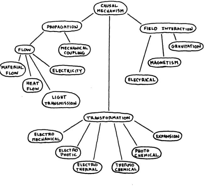
4.1 The Set of Causal M echanisms ... ... 28
4.1.1 Propagations ... 29
4.1.2 Transformations ... 30
4.1.3 Field Interactions ... 32
4.1.4 The Generalization Hierarchy ... 32
4.2 Looking to Physics: Conservation ... 33
4.3 Indexing the M echanisms ... ... 35
5. Levels of Abstraction ... 7
5.1 Levels of Explanation in the Domain Theory ... 37
5.2 A Continuum of Explanations from Empirical to Proven ... 38
5.3 Some Properties of Explanation ... 39
5.3.1 Instantiability ... 40
5.3.2 O bservability ... 40
5.3.3 Consistency ... 41
5.4.1 Controlling the Level of Explanation ... ... 41
5.4.2 Controlling the Level of Perception ... 43
5.5 Summary ... 44
6. Learning from Experiments ... 46
6.1 Experiments Based on Knowledge of Functional Dependencies ... 47
6.1.1 Am biguity in Experim ents ... ... 47
6.1.2 Experiments Based on Transitions ... 49
6.1.3 Experiment Design via Constraint Back-Propagation ... 49
6.1.4 Am biguity Again ... ... 51
6.2 Experiments Based on Knowledge of Causal Mechanisms ... 51
6.2.1 Uninstantiable and Uncertain Experiments ... 53
6.2.2 Experiments for a Single Hypothesis ... 54
6.3 Sum m ary ... 54
7. Constructing, Using, and Refining Causal Models ... 56
7.1 Specifying the Causal Reasoning Task ... ... 56
7.2 The Causal Modelling Procedure ... 57
7.3 Constructing a Causal M odel ... ... 59
7.4 Using and Refining a Causal Model ... 68
8. Sum m ary ... 69
8.1 Relation to Other W ork ... 69
8.1.1 Qualitative Reasoning about Physical Systems ... 69
8.1.2 Empirical and Analytical Learning ... 71
8.1.3 Levels of Abstraction ... ... 71
8.1.4 Learning from Experim ents ... 72
8.2 The Issues Revisited ... 72
R eferen ces ... 74
Appendix A. The Qualitative Calculi ... 76
A.1 Calculi for the Signs of Quantities ... ... 76
A.1.1 Signs under Negation ... ... 76
A.1.2 Signs under M ultiplication ... ... 76
A.1.3 Signs under Addition ... ... 77
A.2 Calculi for the Transitions of Quantities ... 77
A.2.1 Transitions under Negation ... 78
A.2.2 Transitions under Multiplication ... 78
Chapter 1
Introduction
1.1
The Problem, the Motivation, and the Domains
One of the most important skills underlying common sense is the ability to recognize, describe, and reason about regularities and dependencies in the world in terms of causal relations. Causal descriptions enable us to generate useful explanations of events, to recognize the consequences of our actions, to reason about how to make things happen, and to constrain our theorizing when unexpected events occur, or expected events do not occur. The ability to identify causal relations and to construct causal descriptions underlies our ability to reason causally in understanding and affecting our environments.
Imagine waking up in the morning to find the refrigerator door ajar. It is not hard to understand why the food is spoiled, even if one is not quite awake. People commonly turn down the volume control on the home stereo before turning the power on, anticipating and knowing how to prevent a possibly unpleasant jolt. When the flashlight does not work, we will sooner or later check the batteries.
The causal reasoning tasks implicit in the scenarios above include ezplaining the spoiled food; predicting a possible consequence of flipping the power switch on the stereo and planning to prevent that event; and diagnosing the faulty behavior of the flashlight.
Before any of this useful causal reasoning can take place, the causal descriptions which support it have to be constructed or learned. Often they are not available, complete and appropriate for the problem at hand. Instead these causal descriptions have to be proposed on the basis of observations of the system to be understood and perhaps knowledge already in hand about such systems. The problem of causal modelling - the recognition and description of causal relations - in the context of a causal reasoning task is the competence which is the subject of this thesis investigation.
The class of domains which will test the principles emerging from this research effort, and the implementation based on them, is that of physical devices and gadgets - simple designed physical systems. Examples are cameras, showers, toasters, and air conditioners.
Causal reasoning is very important in domains like these. A photographer knows he or she has just wasted time setting up a shot when he or she notices that the lens cap was on when the shutter clicked. The light which would have created an image on the film never reached the film. Someone
drawing a bath knows lie or she can leave the room to attend to other affairs because the safety drain will prevent overflow of water onto the floor. Someone who drops some bread into the toaster and starts reading the morning paper may, after a while, not having heard the toast pop up, check if the toaster is plugged in.
The reasoning outlined in each of these scenarios is supported by a causal model of the particular physical system involved. I propose to show how these causal models can be acquired in the context of a causal reasoning task. The causal reasoning task serves both to constrain the learning task, and to demonstrate that the learning does indeed produce useful causal descriptions.
1.2
The Issues
There are several issues associated with the causal modelling competence. This research will address these issues and attempt to provide principled solutions to them. Indeed, any performance results I present will be suspect if they are not accompanied by such general arguments.
" When/how to construct multi-level causal descriptions/explanations?
Physical systems usually admit to description at more than one level of abstraction. Obser-vations also come at various levels of granularity. I want my learning system to be able to construct causal descriptions at different levels of abstraction. I also want it to be able to de-termine when it might be useful/necessary to examine or explain a physical system at a finer level of detail. The causal reasoning task motivating the learning task can help to determine to what level explanation and perception should go.
* How to learn from experiments?
The ability to design experiments to test and distinguish hypotheses is useful to a learning system. My example-driven inductive inference method can benefit from an analysis of the current set of hypotheses to determine what next example can maximally distinguish the hypotheses. Also, my domain theory can be exploited to determine what next observation can lead to more justified causal hypotheses.
* What kinds of causal relations exist in the physical system domain?
This issue is a knowledge engineering issue. The result of the knowledge enginnering is the domain theory that guides the learning system. I assume that this domain theory is not necessarily complete or consistent. I have looked to the field of physics to ensure that the domain theory has some basis, and is not simply ad hoc.
* How to learn new compositions of causal relations for the domain?
This issue concerns extending the domain theory which drives learning. I show how new, composed causal relation types for the domain can be acquired through an explanation-based learning technique. This approach does not support acquisition of new primitive causal relation types.
* How can empirical and analytical learning techniques complement each other?
Although this research was originally motivated by the specific problem of learning causal models, some issues have arisen that are relevant to learning in general. In particular, my
learning systen combines inductive and deductive inference and has both empirical and ana-lytical learning components. I attempt to step back from the specific interactions of inference
methods and learning paradigms in my system, and considcr whether there are principled ways
of combining these approaches.
What is a good representation for causal relations?
Choice/design of a representation language is an important step in the construction of any
learning system. I have looked to the field of philosophy to come up with a model of causality; this model has guided my design of representations for causal relations. The representations, in turn, have more or less suggested inference methods, both inductive and deductive, which drive the learning of causal models.
1.3
The Learning Tasks
The primary learning task of my system is to construct causal models of physical systems to support a given causal reasoning task. The models are constructed from observations of the physical systems and from knowledge of the general form of causal relations and of the kinds of causal relations that exist specifically in the physical system domain.
The primary learning task is, more formally,
Given a causal reasoning task concerning a physical system, construct a causal model which supports the causal reasoning task, as follows:
* Given structural and sequence-of-events behavioral descriptions of a physical system,
* Hypothesise causal relations which can account for the observed behavior, and when possible, * Justify proposed causal relations by determining if their types of interaction and supporting
system structure indicate a known causal mechanism.
This primary learning task is supported by a background learning capability. The task of this second learning component is to identify and generalize compositions of the known causal mecha-nisms in the causal models produced by the primary learning component. These new, composed causal mechanisms can then be incorporated into the domain theory which drives the first learning component, enhancing its performance.
The secondary learning task is, more formally,
Given a causal model,
* Identify within the causal model new compositions of known causal mechanisms.
* Generalize these new composed causal mechanisms by generalizing their components without violating the constraints of the composition.
aSEAVATIONS
CAUSAL CAUSAL
FMGoELLIN]
I ch IANgIMSYSTEM COHPOSI ION0
SYSTEM
Figure 1.1: The Learning Systems
* Add the composed causal mechanisms and their generalizations to the set of known causal mechanisms.
This secondary learning system falls into the class known as Learning Apprentice Systems. These are learning systems which lurk in the background of other AI systems, extending their knowledge bases by monitoring and analyzing the activities of the systems (and perhaps the users) whose shoulders they are looking over. In my setup, the Learning Apprentice System identifies and gener-alizes justified compositions of causal mechanisms in the causal models constructed by the primary learning system.
1.4
A Scenario
-
The Camera Domain
This section contains a brief outline of the steps my learning system goes through in constructing a causal model of a camera to support the causal reasoning task of how to control the exposure of photographs (a plamling problem). I give some hints of the kinds of knowledge it brings to bear and the inferences it makes in performing this learning task.
The learning system's initial observation of the camera includes a description of the various physical objects that make up the camera system and structural and geometrical relations between these objects.
... The lens, the flash, and the release button are attached to the camers. The aperture ring and the focus ring are attached to the lens.
The film is inside the camera. ...
This structural description is complemented by a behavioral description which tells how the structural and geometrical relations, as well as the values of quantities of the objects, change over time.
... Initially, the
f-stop
of the aperture ring is 5.8. The distance of the focus ring is 8 feet.The intensity of the flash is dark. ...
... Next, the intensity of the subject is bright. The position of the release button is down. The intensity of the flash is bright. ...
... Later, the film is outside the camera.
The film is overexposed. ...
At first, almost any hypothesis about what could be affecting what is supported. The only con-straints in force are that effects cannot precede their causes and that values and relations established by external actions must be primitive causes.
Already though, some hypothesized interactions have the earmarks of causal mechanisms that the learning system knows about. The simultaneous brightening of the flash and the subject could be light transmission. Covering up the flash might be a useful experiment.
Some of the proposed causal relations cannot be instantiated as instances of known causal mech-anisms, either because the relevant mechanisms are unknown, or they can not be observed. For these uzinstantiable causal relations, the learning system can still gather further empirical evidence by performing know-tweaking experiments. This evidence can strongly suggest, for example, that the setting of the aperture ring seems to affect the fihn exposure, while settings of the focus ring do not.
Eventually, when the learning systerii can distinguish or characterize its hypotheses no further, and there is strong empirical evidence for some causal relations, it should be motivated to look inside the camera. Perhaps mechanisms will be revealed which can justify the causal relations which have only an empirical basis. After opening the camera, the learning system can in fact instantiate a mechanical coupling between the aperture ring and the iris in the lens, indicated by the simultaneous changes in position or shape. It can also note a light path between the subject and the film and note that the iris and the shutter control the flow of light along this path.
As a final step, the learning system might note how the f-stop can affect the film exposure via interacting mechanical coupling and flow mechanisms. This complex mechanism might appear in other physical systems and should be incorporated into the learning system's domain theory.
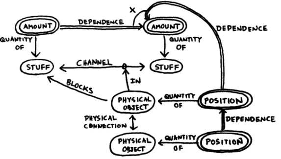
This scenario reveals some of the sources of constraint my learning system employs and some of the reasoning it uses in constructing causal models. The number of hypotheses the learning system may entertain at various times is only suggested. A simplified version of the causal model of the camera which is the output of the learning system appears in the following figure.
The learning task cannot be considered complete until the constructed causal model can be shown to support the original planning problem of how to control the exposure of photographs. Planning involves finding sequences of operations which achieve a goal. When the causal model has revealed chains of causality which originate in available operations (e.g., setting the aperture ring) and terminate in the specified goal (values of the film exposure), then the learning task is complete. The causal model above can be used to generate plans for controlling exposure.
Figure 1.2: A Causal Model
Chapter 2
What is Causality?
In order to convincingly address the issues underlying this research into the causal modelling com-petence, I have looked to the field of philosophy for ideas on what exactly is the concept of causality. The theory of causality which I have adopted is due to Mackie [Mackie 74]. In his theory, causation has three aspects, regularity, direction, and mechanism. Regularity and direction are necessary ex-plicit attributes of any causal relation, while mechanism is not. Regularity refers to the consistent repeatability of an observed co-occurrence of a cause (an event, a state, a relation, or some collection of them), and an effect (similarly defined). Direction refers to the cause being always somehow prior to the effect.
Causal relations which incorporate regularity and direction may be called the associationist causal relations. They are based purely in empirical evidence of an association that always has been observed to hold. However, some causal relations also incorporate a notion of mechanism, which gets at the question of why the effect should necessarily follow from the cause, or what is the tie, or process, by which the cause produces the effect. This notion of necessity is common to all causal relations, but the mechanistic causal relations are the only ones which make the justification for it explicit.
2.1
Causal Direction
Causal relations always have a direction. An effect never precedes a cause. This property of causal relations is based partly in temporal direction. If event A occurs at time t, and event B occurs at time t + 1, then A must be the cause. But causal direction does not arise solely from temporal direction for often events which are perceptually simultaneous can be separated as to which is cause and which is effect.
The competence of identifying causal direction may also make use of knowledge (perhaps heuris-tic) about primitive causes. These are events which are taken to be always external inputs to a system. An example of an event which is a primitive cause is the action of an agent on a physical system. I
IThis may not be a primitive cause in a domain where there are causal interactions among agents; e.g., one agent may "cause" another agent to perform some action.
Thus the direction of causality between two causially linked events can be determined in several ways:
I. The cause is the ievent which is temporally prior to the other. 2. The cause is the event known to be a primitive cause.
3. The cause is the event which is causally linked to an event which satisfies any of these three conditions.
This analysis in no way closes the book on the origins of causal direction. In fact, it somewhat begs the question because primitive causes are defined only extensionally, i.e., no way is given of identifying primitive causes not known a priori.
2.2
Mechanistic vs. Associationist Causal Descriptions
A causal description should have more than an empirical basis; it should do more than associate some set of conditions or changes - the cause, with another - the effect. A causal description also should provide a mechanistic explanation of why the observed interaction occurs. Such an explanation should answer questions like: "What is the medium which supports the causation?", "What kinds of barriers can prevent the interaction from taking place?", and "What class of causal mechanism or process does this interaction fall into?"An associationist explanation of why the film in a camera came out blank might be: "One of the conjunctive preconditions for the dependence between the brightness of the subject and the intensity value on the negative, namely the lens cap being off, was unsatisfied." A mechanistic explanation might be: "The camera works by providing a controlled channel through which light may flow from the subject to the film. In this case, the lens cap acted as a barrier, preventing light from reaching the film."
The associationist explanation can be justified by noting that the film comes out blank/non-blank whenever the lens cap is on/off the lens. But there may be other statements whose truth-value is correlated, perhaps coincidentally, with the exposure or non-exposure of the film. Perhaps the camera was always on/off a tripod when the film came out blank/non-blank. The associationist description cannot further distinguish the lens cap and the tripod as being possible preconditions.
However, a mechanistic explanation of the lens cap in terms of a barrier to a light path does distinguish it a priori from the tripod. Such an explanation of the tripod is not forthcoming.
Associationist descriptions are restricted to aspects of the form of a causal relation: conjunctive or disjunctive, necessary or sufficient, the number of contributions, the sign of a dependence. They can never be supported by anything more than empirical evidence. On the other hand, mechanistic descriptions involve concepts like media supporting causation and barriers inhibiting causation. They provide hooks into domain knowledge, knowledge that can justify the proposal of a causal relation by revealing the a priori known mechanism that underlies the causation. An empirical, associationist causal description can never be justified in this way.
2.3
What is a Causal Mechanism?
I have spoken of mrchanistic descriptions of causal relations without being entirely clear on what I mean by "mechanistic." Roughly, I mean causal descriptions which say something about what is the tie between the cause and the effect? What is it about the cause and perhaps the immediate enviromnent which produces the effect?
These questions get at what philosophers call the necessity of causes. This necessity, if detectable, gives license to the inference that the cause, in the right circumstances, always results in the effect. It is exactly this necessity which a mechanistic causal description is intended to reveal. This is the primary reason why a purely associationist representation of causal relations, which lacks this necessity, is inadequate. Such a representation may capture the form of a causal relation, but it says nothing about why the effect should and does follow from the cause.
A causal mechanism, to be called a mechanism at all, must describe some kind of process by which the cause produces the effect. Examples of processes are flow of material, transfer of momentum from one object to another, expansion of a material, transformation of electrical energy to light, heat, or motion. Processes, in turn, need some kind of medium, or structural link between the cause-object and the event-object, through which the interaction occurs. For example, flow of material requires a channel of some sort while transfer of momentum needs a physical connection between the objects. A complementary notion to medium is that of barrier. Whereas a medium is the structural link which enables a causal mechanism, a barrier is a disruption of the structural link which disables the causal mechanism. A channel can be nullified by a blocking of some kind which prevents flow. A physical connection which is broken cannot transfer momentum.
Processes reveal that there is considerable continuity between perceptually distinct causes and effects. They remove the mysteriousness that sometimes might be associated with a causal link. Processes typically describe a kind of persistence as well; some quality or form, present in the cause, is still present in the effect, although this persistence may not be always immediately perceivable.
A few examples of causation in physical systems and their mechanistic descriptions are illustrative here: A flashlight is turned on and a wall across the room brightens. The mechanistic explanation is that the flashlight emits light which flows through the intervening space to fall on the wall and brighten it. The cause-event and the effect-event are the changes in brightness of the flashlight and the wall, respectively. The medium is the straight-line, unobstructed path between them. The mechanism itself, or the process, is the continuous flow of light radiation from the flashlight to the wall. Finally, there is a persistence, or conservation of form, across the cause and effect; both involve changes in brightness.
Another example. The faucet in a shower stall is turned and momentarily, water emerges from the shower head. The mechanistic explanation runs thus: The faucet is connected to a pipe which runs to the shower head. Turning the faucet opens a valve in the pipe, allowing water to flow to the shower head and emerge there. There are two causal mechanisms involved. First, there is a mechanical coupling between tile faucet and the valve. Turning the faucet results in movement of the valve. A physical connection, perhaps a rod, acts as medium here. The valve itself is a removable barrier to the flow of water to the shower head. This flow is the second causal mechanism. The pipe is the medium through which the flow occurs. In both of these causal mechanisms the cause resembles the effect. A movement of the faucet at one end of a mechanical connection is transferred to the other end, resulting in movement of the valve. A change in amount of water at one end of a
The flashlight, straight-line path, and wall make up a system of light transmission. The faucet, rod, and valve comprise a mechanical coupling. The pipe and shower head are only part of a larger system of water transport, which includes a water source somewhere up the line.
There are appropriate barriers which could have disabled each of these causal mechanisms. The flashlight would not have brightened the wall if an opaque card was held in front of it. Turning the faucet would not have moved the valve if the rod was broken. And water would not reach the shower head if the pipe was clogged.
Each causal interaction consisting of a cause-object, medium, and effect object helps to locate the boundaries on the closed system inside which events can affect one another. This is roughly the spatial part of Pat Hayes' notion of causal enclosure, which he calls history [Hayes79]. What barriers do, cssentially, is chanlge the boundaries on the closed systems within which causal interactions occur. The flashlight does not stop emitting light, but it only brightens the card. Turning the faucet does move the rod, but only up to the break. And water flows to the clog but no further.
To summarize the notion of causal mechanism developed in this section: A causal mechanism describes how a cause-event propagates through some medium via some process, in the absence of relevant barriers, to produce an effect-event. The identified cause, medium, and process comprise a sufficient causal explanation for the observed effect, in that they provide a full accounting of why the cause, in these such and such circumstances, should result in the effect. This elaborate description goes further than any. associationist causal description could; it reveals what is the tie, the philosophers' necessity, between cause and effect.
Chapter 3
Representations for Causality and
Methods for Generating Empirical
and Justified Causal Hypotheses
All learning systems are ultimately limited by the representation languages they use. A learning system cannot learn what it cannot represent. An important part of this research is the design of representations for causal relations.
I present both associative and mechanistic representations for causal relations, and inference methods based on them which perform the task of constructing causal models. The associative rep-resentations describe the general form of causal relations and support empirical, inductive inference methods. The mechanistic representation, on the other hand, supports the description of specific types of causal mechanisms which comprise a domain theory of causal relations for physical systems. The inference method which operates on this representation is deductive, and can generate justified hypotheses of causal relations, which the inductive methods can never do.
Although I argue that the mechanistic representation and its deductive inference method are preferable, nevertheless the associative representation and the inductive inference method have their place. This is because the domain theory driving deductive inference has inadequacies. For example, the domain theory is not considered to be complete. There may be causal mechanisms which operate in the domain which are unknown. The deductive method would fail utterly in its attempt to recognize an instance of an unknown causal mechanism. On the other hand, the inductive method, which does not utilize the domain theory, is unaffected by its incompleteness, and could still generate hypotheses purely from empirical evidence.
3.1
A Boolean Representation for Causality
I begin my survey of representations for causality and inference methods which operate on them by considering the work of John Stuart Mill, a philosopher who worked on the causal induction problem
Figure 3.1: A Simple Boolean Representation for Causality
~N
oToCAUSE
• •o'€
Figure 3.2: A Better Boolean Representation for Causality
A single cause (a condition, an event) results in an effect.
In an inductive context, the only constraints available for exploitation are regularity and direc-tion. If the effect does not occur every time the suspected cause does (but not necessarily vice versa), then the correct cause has not been found.
This representation is too simplistic for several reasons. Causes typically do not cause in a vacuum. There is usually a set of relevant enabling preconditions which must be satisfied to bring about an effect. Or, there may be several disjoint ways in which an effect can be produced. Finally, it may be the absence, rather than the presence of some condition which brings about an effect.
A more sophisticated representation of causal relations would allow arbitrary conjunctions, dis-junctions, and negations in the cause. Also, the cause may be considered necessary, or sufficient, or
both for the effect.
3.1.1 Mill's Methods of Causal Induction
Mill formalized a set of methods of causal induction which operate on this general boolean repre-sentation for causal relations. Perhaps the most interesting aspect of his work is his careful analysis of the interactions between assumptions. observations, and inductive inferences. A more accessible account of Mill's methods may be found in the appendix to Mackie's book on causation [Mackie 74]. The examnples to come are drawn from Mackie.
To illustrate Mills's methods of causal induction, consider the following example. Suppose that A, D, C, and D are possible causes I of E and we have the following observation.
OBSERVATION A B C D E
Examnple 1 T T F ? T
Example 2 F T ? T F
There is one positive example in which the effect E occurs, and one negative example in which it does not. The inductive task is to determine what cause for E was present in the positive example and absent in the negative one.
If we assume that some single, unnegated condition is necessary and sufficient as a cause for E then we can conclude that A is this cause. D and D are eliminated because their presence in the negative example, when the effect did not occur, shows they are not necessary. C is eliminated because its absence in the positive example shows it is not sufficient.
If instead we assume that a cause may be negated, i.e., the absence of some condition may be the relevant cause, then the observation above camlot eliminated C and D. We need a stronger observation which shows that C was false in both examples and D was true in both.
If we relax our assumption about the form of the cause to allow conjunctions (with unnegated conjuncts), then the hypotheses AD, AD, and ABD must be kept under consideration. We can conclude that A is necessary, but perhaps not sufficient.
The interactions between assumptions, observations, and inductive inferences become more com-plex as we admit various combinations of negations, conjunctions, and disjunctions. In general, the weaker the assumption (the greater the number of possible forms for the cause), the more under-constrained the conclusion, given the same observation.
The manipulation of assumptions and inferences is familiar to the AI community as non-monotonic reasoning [Doyle 791. The role of assumptions in inductive reasoning specifically also has been treated
[Utgoff 85). What is impressive about Mill's work, and perhaps sobering for AI researchers, is that he was attentive to the need for making assumptions explicit and was able to analyze the consequences of manipulating them. In the context of his methods of causal induction, he made a quite complete treatment of these issues.
3.2
A Representation for Causality Based on Quantities
and Functional Dependencies
In the representation scheme for causal relations outlined above, the conditions, events, and/or changes which make up causes and effects are represented by statements which are true or false. This is an inadequate representation for describing the physical systems which my learning system will investigate. In particular, there is no easy way to describe the continuous properties of objects in such systems, properties such as height, temperature, velocity, etc. In the boolean representation, we would have to say that at any time, one possible value of a quantity was true and all others were false. An awkward representation.
Instead, I have adopted Forbus' qualitative representations for quantities, their value spaces, and functional dependencies between them [Forbus 84]. These form the basis for another associative representation for causality which supports inductive inference. This representation is designed to easily capture the kinds of continuous phenomena that occur in physical systems, which the boolean representation could not.
D brought under suspicion as possibly participating in a cause for 8 in the first place? The inductive methods given in this section provide no handle on this issue. I return to it later.
DEPENDENCE
>
Figure 3.3: A Simple Representation for Causality Based on Functional Dependencies
3.2.1
Another Set of Methods of Causal Induction
The task now is to develop a set of inductive methods which operate on the representation for quantities and dependencies. The inductive method presented in this section is an expanded version of work done in my master's thceis [Doyle 84].
In this new representation, the simplest kind of causal relation is a single direct proportionality relation between two quantities: y = p(x). To make life as simple as possible, we can assume further that the proportionality relation is monotonic and that the zero values of the two quantities coincide
(i.e., y = 0 when x = 0).
The single direct proportionality assumption under the functional dependencies representation of causality is analogous to the single unnegated cause assumption under the boolean representation.
The inductive task is also correspondingly simple.
For example, consider the following set of observations. Observations under the new representa-tion consist of the signs of quantities. 2
OBSERVATION A B C E
Example 1 + - 0 0
Example 2 + - + +
Example 3 + 0 + +
Under the single direct proportionality assumption, causes (independent quantities) are those quantities whose signs are always the same as the sign of the effect (dependent quantity). In the example above, with this assumption, only C could be a cause of E.
This representation of functional dependencies is too simplistic. Just as we were forced to consider various compositions of negation, conjunction, and disjunction under the boolean representation, now we must consider compositions of functional dependencies under negation, multiplication, and
addition.
Allowing negation admits the possibility of inverse proportionality relations: y = -p(z). The following table shows how the signs of quantities are transformed under negation.
asign -aign
0 0
+
- -+
Thus a negative dependent quantity can now result in two ways. A direct dependence and a negative independent quantity, or an inverse dependence and a positive independent quantity. This
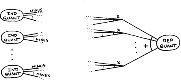
QU Nos
NUs"
Figure 3.4: A Better Representation for Causality Based on Functional Dependencies
loosening of the assumptions about the form of the cause does not admit any further hypotheses for the observation above, but it might have. In particular, a quantity whose signs in the three observations above were 0,-,-, respectively, would now have to be considered as a cause for E.
As long as we assume that only one independent quantity is affecting any dependent quantity at any time, the inductive task is still highly constrained. This is the analog of the single cause assumption for the boolcan representation of causes and effects.
Once we relax the single-cause assumption by admitting multiplication and addition, things become more complicated.
We need to describe how contributions of several functional dependencies combining multiplica-tively can affect the values of dependent quantities. The arithmetic form of this type of multiple functional dependence is y = pi(zX) x p2(z2) x .. p- ,,(,). Combinations of the signs of two contri-butions under multiplication are listed in the following table.
signi sign2 signs x signs
0 0 0 + 0 0 - 0 0 0 + 0 + + + - + 0 - 0 +--- +
These two-operand combinations can be applied recursively 3 to determine how several contribu-tions combine multiplicatively. Alternatively, this knowledge can be aggregated to the general case of n contributions a priori, as has been done in the following table.
signs = 0 signs = + signs = - signs x sign2 X ... x sign.
>1 >0 >_0 0
0 > 0 even +
0 > 0 odd
3
1n any order, since multiplication is communutative and asociative.
Using this knowledge of how contributions combine under multiplication we find that there are now more causal hypotheses that are consistent with the given observations, namely A x C and (-A) x (-C).
Now we consider multiple functional dependencies of the form y = pi(zl)+p2(zX)+... +pn(,). Combinations of the signs of two contributions under addition are listed in the following table.
sign, sign2 sign, + aign2
0 0 0 + 0 + - 0 0 + + + + + - + 0+-0 - -+ -
0+-Again, we can compute combinations of n contributions under addition by applying the two operand combinations recurisively. Or we can aggregate the knowledge a priori as in the following.
signs = 0 aigns = + signs = - sign, + sign2 + ... + aignn
>0 0 0 0
>0 >1 0 +
>_0 0 >1
>0 >1 >1
0+-Notice the ambiguity when contributions of opposite sign are added together. This indeter-ininism makes the additive induction problem inherently less constrained than that of negation or multiplication.
Armed with this knowledge of how contributions combine additively, we must now consider the following causal hypotheses, given the above observations: A + B, A + B + C, and A + B + (-C).
Finally, we can consider the most general case, that of arbitrary compositions of negation, multi-plication, and addition. Again, we can determine which compositions are consistent with the given observations by applying the appropriate combinations from the tables for negation, multiplica-tion, and addition recursively. The hypotheses which now have to be admitted are (A + B) x C, (A + B) x (-C), and ((-A) + (-B)) x (-C).
Transitions
This new set of inductive methods operate, like Mill's methods, through elimination of hypotheses. Hypotheses which do not satisfy constraints which specify the valid combinations of functional dependencies under negagtion, multiplication, and addition are removed from consideration. The constraints I have described so far concern how the Rigns of quantities from individual observations must combine under these operations. This is not the only source of constraint which can drive these inductive methods. Also of relevance are the ways in which the values of quantities change from one observation to the next. For example, a quantity whose value was positive in two successive observations may have actually decreased, stayed the same, or increased. These transitions also combine in well-defined ways wider negation, multiplication, aid addition. The value of specifying
S ST-AY+aSTY ) ADD+ EN AILE 4- ADD- ENABLE-TC JJr f.5E 4 SUTRACT 4+ DISASLE - SUrTPLAC(T- DISCISLE-RE r
L6E-Figure 3.5: The Transitions
the exact transitions is that not all of them may be consistent with the given observations. Knowledge of transitions also can drive these eliminative, inductive methods.
The following table and above figure define the possible transitions of quantities between succes-sive observations.
Transition New Direction of Abbreviation
STAYO STAY+ STAY-ADD+ ADD-SUBTRACT+ SUBTRACT-ENABLE + ENABLE-DISABLE+ DISABLE-REVERSE + REVERSE-sign 0 change 0 0 0 STO ST+ ST-+ + + AD+ -- - AD-SB+ SB-EN+ EN-DB+ DB-RV+
RV-The calculi which describe how these transitions combine under negation, multiplication, and addition appear in the appendix.
This knowledge of transitions and how they combine umder negation, multiplication, and addi-tion now can be used to make further inductive inferences. Observed transiaddi-tions can be combined recursively according to the operations specified in the various causal hypotheses. The closures of the transitions of the causes (independent quantities) under the compositions specified in an
hy- StAY-STAYO
pothesis nmust contain the observed transition of the effect (dependent quantity) for all observations;
otherwise that hypothesis cannot be considered viable.
3.2.2
Examples of Inductive Inference
Consider again the earlier set of observations, now extended to include not only the signs of quantities in each observation, but also the transitions of quantities between observations.
OBSERVATION A B C E
Example 1 + - 0 0
Transition 1--2 AD+ ST- EN+ EN+
Example 2 + - + +
Transition 2-+3 AD+ DB- SB+ SB+
Example 3 + 0 + +
Recall that one of the hypotheses that survived the earlier inductive inferences was (A + B). Now we show that this hypothesis can be eliminated because the observed transitions are inconsistent with the form of (the composition of operators specified by) this hypothesis.
Quantity A underwent an AD+ transition from example 1 to 2. Quantity B underwent a ST- transtion from example 1 to 2.
The combination of AD+ and ST- under addition is (AD+ SB- EN+ DB- RV-).
The transition of the dependent quantity E from example 1 to 2 is EN+ which is in this closure. The hypothesis is still viable.
Quantity A underwent an AD+ transition from example 2 to 3. Quantity B underwent a DB- transtion from example 2 to 3.
The combination of AD+ and DB- under addition is (AD+ SB- EN+ DB- RV-).
The transition of the dependent quantity E from example 2 to 3 is SB+ which is not in this second closure. The hypothesis can now be eliminated.
Interestingly, the hypothesis (A + B + C) does survive this analysis.
Recall that the set of possible transitions of (A + B) from example 2 to 3 is (AD+ SB- EN+ DB- RV-).
Quantity C underwent a SB+ transition from example 2 to 3.
The combination of (AD+ SB- EN+ DB- RV-) and SB+ under addition is (STO ST+ ST- AD+ AD- SB+ SB- EN+ EN- DB+ DB- RV+ RV-) - all possible transitions. This hypothesis cannot be eliminated.
Continuing this analysis, the final set of hypotheses consistent with the given observations is C, A x C, (-A) x (-C), (A + B + C), (A + B) x C, (A + B) x (-C), and ((-A) + (-B)) x (-C).
The knowledge about how signs and transitions combine under negation, multiplication, and addition makes up a kind of qualitative calculus which can be exploited to make inductive inferences.
This knowledge reveals two sources of constraint. There are a limited number of ways in which the signs of several contributions due to functional dependencies on a quantity can combine to produce the sign of that quantity. And there are a limited numbcr of ways in which changes in the underlying contributions on a quantity can combine to produce changes in that quantity.
3.2.3
Qualitative vs. Quantitative Values
My set of inductive methods is driven by observations of the qualitative values of quantities. It is important to point out that qualitative vawues inherently carry less constraint than quantitative values. For examnple, ml hypothesis involving two additive contributions, one of +4 and one of -2, say, can be eliminated as a possible explanation for a value of +3. On the other hand, if we know only the signs of these values, this hypothesis cannot be eliminated.
One valid characterization of my inductive method is that it is a qualitative version of a program like BACON [Langley et al 83), which performs quantitative function induction. Given quantita-tive observations, it is true that a quantitaquantita-tive induction method would outperform my qualitaquantita-tive method because it would make use of additional constraint to eliminate hypotheses more effectively. However, I am assuming that my learning system will have access to qualitative values only. Specifically, the learning sytem will know the signs and the relative magnitudes of different symbolic values for quantities, i.e., whether the value of a quantity is greater than, less than, the same as, an earlier value of the same quantity or a value of another quantity of the same type. I think this is a realistic assumption for any Al system in a simulated (or real) visual environment. I do not assume
the existence of perceptual equipment that can quantize observations.
3.2.4
Assumptions and Inductive Inferences Again
Mill's inductive methods can make inductive inferences only relative to assumptions about the form of boolean causal relations - in particular, whether negations, conjunctions, and/or disjunctions were to be admitted. Similarly, the set of inductive methods outlined above - based on a quanti-ties and functional dependencies representation of causal relations - can make inductive inferences only relative to assumptions about how these causal relations might combine. Now the possible combination operators are negation, multiplication, and/or addition.
There are other assumptions we might make within the quantities and functional dependencies representation which can eliminate some hypotheses and hence constrain the induction problem.
For example, we might assume that there are never contributions in opposing directions (both + and -). Or we might assume that in the case of additive contributions, the equilibrium state is stable and robust, i.e., that opposing contributions always relax to the equilibrium state. Another possibly reasonable assumption is that the equilibrium state is unattainable. Yet another is that multiplicands never can be negative, so that quantities can only be amplified and reduced via multiplication by non-negative values.
These possible assumptions can apply equally, in most cases, to the signs of contributions and their combinations and to transitions of contributions and their combinations. For example, the no equilibrium assumption applied to transitions of contributions means that transitions cannot cancel out under addition, i.e., combinations such as ADD+ + SUBTRACT+ -* STAY+ are disallowed.
Another assumption, more subtle than the others, has to do with knowing the zero points of proportionality relations. As mentioned earlier, we asnsume by default that for any proportionality
relation y = p(z) (or y = -p(z)), y = 0 when z = 0. This need not be the case. Yet not knowing where these zero points are means it is impossible to determine whether a contribution is null,
positive, or negative. 4
Similarly, it is impossible to determine which of several transitions of the same direction of change is the correct one. Without some assumption about where zero points are, there is no alternative but to consider all possibilities for the signs and transitions of contributions - a severely underconstrained induction problem.
Yet another insidious assumption, one which is inescapable because of the impossibility of con-firming hypotheses through induction, is that all relevant causes (independent quantities) are being considered. If this asstumption is violated, there may be no hypotheses which are consistent with observations. This would be the case if the quantity C was ignored in the above observations.
One reason why a relevant independent quantity might be ignored is because it cannot be ob-served at the given level of perceptual granularity. It is possible to propose hypotheses which include "ghost" or hidden quantities and test them with the inductive methods I have outlined. This, too, leads to a terribly underconstrained induction problem because, clearly, all possibilities have to be considered for the signs anid transitions of hidden quantities.
All of these assumptions are posable and retractable in the non-monotonic reasoning sense. They constrain the number of hypotheses which have to be considered either by affecting the number of valid combinations of functional dependencies, or by affecting the number of valid interpretations of observations.
Still other assumptions are more or less hard-wired and are not amenable to non-monotonic treatment. One of these assumptions is that all proportionality relations are monotonic. Once the sign of one of these primitive functional dependencies is determined, it is known for all values of the independent quantity. Without this assumption, the best that could be hoped for with qualitative values is to try and isolate intervals in the range of values of the independent quantity within which the sign of the dependence does not change. A recent paper has shown how a conceptual clustering algorithm might be used for this task [Falkenheimer 85].
Another hard-wired assumption is one I call omniregponsivity. This assumption states that all perceivable changes in independent quantities result in perceivable changes in dependent quantities. Combined with the monotonicity assumption, this becomes strict monotonicity combined with a statement about perceptual resolution.
Making assumptions explicit is an important task in building any AI system. Inferences are al-ways affected by assumptions iand it is virtually impossible to design representations and procedures which operate on them which are assumption-free. Non-monotonic reasoning allows some assump-tions to be manipulated. But even for those assumpassump-tions which are hard-wired, exposing them helps to reveal, in turn, limitations of the AI system that uses them.
3.3
A Representation for Causal Mechanism
In this section, I present a representation designed to capture the notion of mechanism which is cen-tral to the concept of causality in physical systems. Knowledge of the kinds of causal mechanisms
4
1 DEPE P4DE rAC
E-M.O
A4ITYL
6
iUAr4TITYOF
I OF
(rOýIlPTsvO31T~cL1 /PHYSCAAL
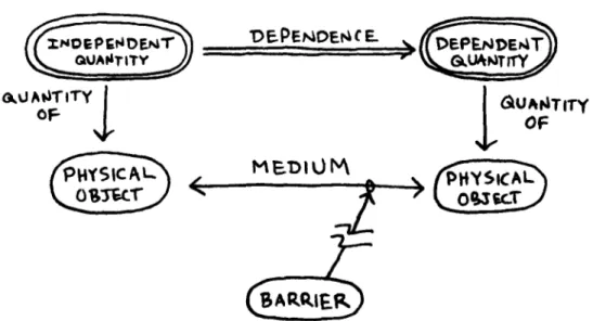
Figure 3.6: A Mechanistic Representation for Causality
that exist in the physical system domain can be described in this representation. The representation supports an alternative, more knowledge-intensive approach to the causal modelling problem involv-ing a deductive metlhod. This inference method generates justified hypotheses of causal relations as instances of known causal mechanisms.
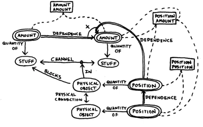
The representation I have developed combines, at the level of form, the boolean representation and the quantities and functional dependencies representation for causal relations. In addition, and most importanutly. it directly incorporates a mechanistic vocabulary. The set of ontological descriptors is extended to include ternis like medium and process, instead of just domain-independent terms like precondition and dependence. Also, physical objects and quantities can be classified, which aids in the recognition of particular causal mechanisms.
This representation can be thought of as a template for causal mechanism schemata. The basic causal relation remains the functional dependence between quantities. Quantities are associated with physical objects, and all can be typed. Processes are essentially typed functional dependencies. There are two kinds of relevant preconditions. One is an enabling condition: there must be a structural link, a medium, between the cause object and the effect object. The other is a disabling condition: there must be no barriers which would disrupt the medium and decouple the cause and effect objects.
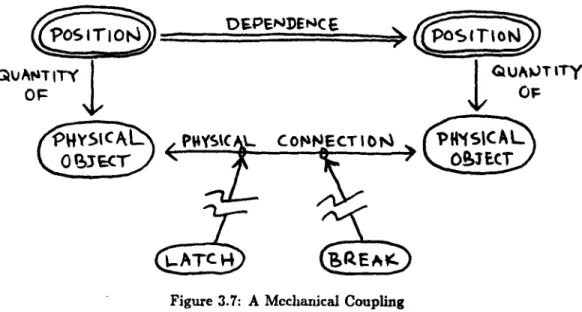
A mechanical coupling is an example of a causal mechanism relevant to the physical system domain which can be described within this representation.
A mechanical coupling is characterized by co-occuring motions of two objects. The relevant quantities are those that describe position. The medium between the objects is some kind of physical connection. A possible barrier is a break in the connection.
The representation for causal mechanism is an abstract structure with objects whose types are quantities, media, barriers, etc. Each causal mechanism described within this representation has the same structure but objects are specialized to particular classes of quantities, media, etc. The domain theory I present later includes not only a set of causal mechanisms for the physical system domain but also a generalization hierarchy for those mechanisms. Part of the domain knowledge is of the generalizations that are possible within the domain.
DEPENDENCE
QUAIJT ITy OF
alA
~SPA1\
(PHYSyCL
COakNEcT
0r4
(IcAlslZ
-ATCH
4REA9
Figure 3.7: A Mechanical Coupling
3.3.1 A Deductive Method
The inference method which operates on the causal mechanism representation is deductive, and is concerned with recognizing proposed causal relations as instances of the a priori known causal mechanisms in the domain. Each causal mechanism description embodies a deductive inference rule of the form:
3(iq)3(dq)3(m)-3(b)
(IndependentQuantityType(iq) A IndependentQuantityType(dq)A
MediumType(m) A Between(m, PhysicalObject(iq), PhysicalObject(dq)) DarrierType(b) A Along(m, b))
= FunctionalDependence(iq, dq)
When a causal mechanism template can be fully instantiated (unified) into an observation, an instance of that causal mechanism is strongly suggested. However, the domain theory is not nec-essarily consistent. There may be exceptions to these inference rules. For this reason, the causal explanations generated from the domain theory are justified, but do not necessarily constitute proofs in the strong truth-prescrving sense.
Sometimes the causal mechanism templates include information about the signs of proportionality relations, which can be instantiated along with the rest of mechanism descriptions. Furthermore, and of more interest, some compositions of causal mechanisms correspond to combinations of functional dependencies under addition and multiplication. The ways in which structural relations in causal mechanisms interact can give clues about how functional dependencies are combining additively or multiplicatively.
For example, several disjoint media adjoining the same physical object may indicate that the functional dependencies supported by those media are combining additively. An example is the several charmels through which water may enter or leave a sink. There is the tap overhanging the basin, the drain at the bottom of the basin, and the safety drain close to the top of the basin. The net change in the level of water in the sink is the sum of the flows, some positive and some negative, associated with these separate media. Since the media, and the contributions, are disjoint, any one is sufficieint to produce an effect. Addition is similar to disjunction in this respect. The definition of media as enabling conditions also suggests this disjunctive property.
Barriers, on the other hand, may indicate multiplicative contributions. Barriers can be thought
of as controlling the magnitude of causal interactions along media, with a complete barrier
corre-spouding to multiplication by zero. For example, a stopper placed over the drain in a sink will change the flow out of the drain by a multiplicative factor. When the stopper is placed securely in the drain, there is no flow. Just as addition bears similarities to disjunction, multiplication resembles
conjunction, in that a single intact barrier can inhibit causation. This is also in keeping with the definition of barriers as disabling conditions.
These observations can be construed as a very simple theory of deriving function s from structure.
I do not claim any definitive, or even terribly insightful contribution to this interesting issue. I
am more interested in how deductive inference, supported by a domain theory, can complement inductive inference. There are ways in which additive and multiplicative contributions might arise other than the ones I have pointed out. For example, addition may occur via integration over time; multiplication may arise via iteration.
3.4
Feature Selection
The methods of causal induction outlined above are based on elimination of hypotheses. The inductive inferences made by the methods implicitly rely on the argument: "These are the only known possible causes which satisfy the constraints imposed by our assumptions about the form of the cause and our set of observations." But there is never a guarantee that the relevant causes have been considered. What is needed is some means of identifying possible causes.
This is the feature selection problem in learning. Inductive methods, in general, do not address it. These methods take as input a set of possible causes (or features), but they do not say how to arrive at this set. On the other hand, the domain knowledge driving the deductive approach to causal modelling does provide a partial solution to the feature selection problem. The domain knowledge is of what kinds of causal mechanisms there are. IKnowledge of these mechanisms with their associated media, potential barriers, and characteristic physical objects and quantities gives the learning system guidance in knowing what is relevant, i.e., what are the possible causes. This knowledge is brought to bear during the generation of hypotheses.
It is important that this knowledge be used only as a focussing, and not an eliminative mechanism. The set of known causal mechanisms for the domain is not taken to be complete; there may be other causal mechanisms which operate in the domain. For this reason, the domain knowledge provides only a partial solution to the feature selection problem. The learning system may have to and should be able to consider causal hypotheses which cannot be justified with the current domain theory.
3.5
Combining Inductive and Deductive Inference
My causal modelling system utilizes both inductive and deductive inference. I have hinted at how these two inference methods interact in my system. Now I step back and consider whether there are principled ways of combining inductive and deductive inference in a learning system.
Inductive inference methods are inherently eliminative, or falseness-preserving [Michalski 83] while deductive methods are truth-preseruing, or confirmative. After an inductive inference, there