Cost and technology assessment of low thrust orbital transfer vehicles

(1)

Cost and Technology Assessment of Low Thrust

Orbital Transfer Vehicles

by

Raymond John Sedwick

B.S., Pennsylvania State University (1992)

SUBMITTED TO THE DEPARTMENT OF AERONAUTICS AND ASTRONAUTICS IN PARTIAL

FULFILLMENT OF THE REQUIREMENTS FOR THE DEGREE OF

MASTER OF SCIENCE

at the

MASSACHUSETTS INSTITUTE OF TECHNOLOGY May, 1994

The author hereby grants to MIT permission to reproduce and to distribute paper and electronic copies of this thesis document in whole or in part.

II

Signature of Author

Deviment of Aeronautics and Astronautics May 6, 1994

Certified by

I

Accepted by

Professor Jack L. Kerrebrock Thesis Supervisor

V Professor Harold Y. Wachman

Chairman, Department Graduate Committee

MASSACHUSETTS _INSTITUTE OF T1N0 t o-9l(wy

'JUN

091994

blWB E~ A rn

/^^

(2)

Cost and Technology Assessment of Low Thrust

Orbital Transfer Vehicles

by

Raymond John Sedwick

Submitted to the Department of Aeronautics and Astronautics on May 6, 1994 in partial fulfillment of the requirements for the degree of Master of Science in

Aeronautics and Astronautics

Abstract

A detailed cost analysis of solar electric orbital transfer vehicles (SEOTV) is performed. Analytic methods for obtaining AV and transfer times for combined orbit raising and inclination change in the presence of shadow are developed to allow

application of the rocket equation to the low thrust transfers. A design space spanned by injected LEO mass, specific impulse, and mass flow rate (thrust) is exhaustively explored to determine absolute minimum launch costs using various launch vehicles, thrusters, and solar cell materials. Solar array degradation is included in the analysis, as well as

opportunity costs associated with long transfer times. Four different mission scenarios including simple delivery, integrating the payload and SEOTV, launching multiple payloads, and reusing the SEOTV are discussed.

Arc jets are found not to offer significant savings over present systems, whereas Hall, Magnetoplasmadynamic, and Ion thrusters are found to offer a great deal of savings

over the present payload ranges, as well as double the maximum payload for the Titan IV, up to 10,000 kg. These same thrusters were found also to permit GEO launches of up to 150 kg for under $23M using the Pegasus launch vehicle. All analyses assume Silicon solar cells, because the present cost of InP and GaAs cells is shown to be prohibitive to their use, except for reusable vehicles which would require the self-annealing properties of InP. Transfer times are on the order of one year, with launch savings from $10M to as high as $160M per launch.

Thesis Supervisor: Dr. Jack L. Kerrebrock

Title: Professor of Aeronautics and Astronautics

Space is big. You just won't believe how vastly, hugely, mind-bogglingly, big it is. I mean, you may think it's a long way down the road to the drugstore, but that's just peanuts to space.

(3)

Acknowledgments

With regards to this thesis specifically, I would like to thank my adviser,

Professor Jack Kerrebrock for his wisdom and enthusiasm in helping me to complete the project on time. I hope he can keep it up for another three year stretch through a PhD. I would also like to thank the various contributors of the information within: Professor Martinez-Sanchez, Mike Fife, Guy Benson, Kim Kohlhepp, Jay Hyman, Bob Beatty, Hughes, Olin Aerospace, and Spectra Gases.

Special thanks goes out to the United States Air Force for their sponsoring of my fellowship for this and the next two years. I hope the work is to their liking.

In addition I would also like to acknowledge the people that make my life such wonderful chaos both in the office and out. First, my friends and officemates of last year, most of who had the audacity to graduate without me: Jim, Chris, John, Pam, Jolly,

Renee, Scott, Eric, Brian, Robie, David, David, Dave, and Dave -- we were plagued with

Daves... and of course, the team of new recruits: Carmen, Guy, Graeme, Jim, Derek, Josh, Gabriel, Dave, Dave, and Dave... these are new Daves.

Upon reflection, I think the only people I've not mentioned are Scott, Chris, Rick, Eric, Brian, Joe, Karen, and of course Celine, who is one of the best friends a person could have. These are friendships I'll always cherish.

While I'm rolling, I would like to thank the Aerospace Engineering Department of Penn State University for bestowing upon me most of the engineering knowledge I have today. Specifically to Drs. David Jensen, Mark Maughmer, Robert Melton, and Roger Thompson, whose letters of recommendation I was constantly requesting have helped me both academically and financially over the years. I hope I don't disappoint them ...

Of course I can't forget to thank my parents, whose love and encouragement (as well as money) have supported me without question since... always. Dad was responsible for my interest in science, and seemed to always have the answers. Mom covered most everything else, and even taught me to cook... sort of. And thanks to my grandma, who entertained me for countless hours with crafts and chocolate chip cookies.

Finally, I would like to dedicate this work to my grandfather, John E. Cockroft who taught me to tinker and build. A fair portion of my life was spent working in his shop, the culmination of a lifetime of gathering tools, equipment... and stuff. He taught

me engineering without the numbers, to adjust the design on the fly -- it wasn't always

(4)

List of Figures

2.2.1 Shadowing of Spacecraft in LEO 18

2.2.2 Modified Thrust Effectiveness Due to Circular Constraining 19

2.2.3 Fraction of Eclipse Time to Total Transfer Time 21

4.1.1 Solar Cell with Concentrator Cover Glass 33

4.1.2 Array Specific Power vs. Time in Orbit 34

5.2.1 Launch Costs Using Arc Jets 45

5.2.2 Launch Costs Using Hall Thrusters 46

5.2.3 Launch Costs Using MPD Thrusters 47

5.2.4 Pegasus Performance for GEO Payloads 48

5.6.1 Launch Cost with Reusable Vehicle 50

A.1 Efficiency Effect on Cost (EOC) 54

A.2 Array Specific Power (EOC) 54

A.3 Solar Cell Cost (EOC) 55

A.4 Payload Value (EOC) 55

A.5 Thruster Cost (EOC) 56

A.6 Interest Rate (EOC) 56

A.7 Structural Cost (EOC) 57

A.8 Mission Control Cost (EOC) 57

B. 1 Inserted LEO Mass vs. Payload to GEO Under Optimal Constraint (UOC) 59

B.2 Specific Impulse vs. Payload to GEO (UOC) 60

B.3 Transfer Time vs. Payload to GEO (UOC) 61

B.4 Power vs. Payload to GEO (UOC) 62

(7)

List of Tables

2.4.1 Launch System Payloads and Costs 26

4.1.1 Comparison of Cell Types Considered 33

4.2.1 SOA High Power Ammonia Arc jet 35

4.2.2 Hall thruster (Stationary Plasma Thruster) 36

4.2.3 Magnetoplasmadynamic (MPD) Thruster 36

4.3.1 Propellant Data 38

4.3.2 Tank Data 38

4.4.1 Typical GN&C Actuators 39

4.4.2 Typical GN&C Sensors 40

4.5.1 Typical S-Band TDRSS User Communication Subsystem 40

4.7.1 Mission Control Estimates 41

(8)

Nomenclature

a ad ah ar a0 B CA Cc CF CGNC CMC Cp CR Cs e ex ey fT h i I Isp KA KF KMc Kp Ks MA Mc Mf MF ML Mo Mp Ms MT MTK rih Semimajor axis N Total acceleration p Normal acceleration Po Radial acceleration N Circumferential acceleration Pp

Borrowed money (principle) P,

Array cost

Communication cost RE

Framework cost RLEo

GN&C cost RT

Mission control cost s

Propellant cost t Cost of repair Shielding cost a Eccentricity o0 X-component of e vector AV Y-component of e vector t_lT Tankage fraction

Specific angular momentum pp

Inclination _PT

Accrued interest a

Specific impulse 'b

Array cost multiplier Ite

Framework cost multiplier I"t

Mission control cost multiplier 0

Propellant cost multiplier Shielding cost multiplier

Array mass g

Communications mass L

Final (dry) mass RGEO

Framework mass Payload mass Initial mass Propellant mass Shielding mass Thruster mass Tank mass Mass flow rate

Number of orbits Orbital parameter

Power usage of other systems Number of orbits

Propellant pressure Power usage of thruster Radius vector

Earth radius Radius of LEO Propellant tank radius Interest rate (percent yearly) Thickness of prop. tank wall

Velocity vector Array specific power Inclination thrust angle Velocity Change Thruster efficiency Subtended shadow angle Propellant density Propellant tank density Propellant tank stress Burn time Eclipse time Transfer time True anomaly 9.81 m/s2 398600 km3/s2 42000 km

(9)

Introduction

With the dawning of the age of the information superhighway, it is becoming increasingly important to establish better and faster communication links throughout the world. This requires the placement of numerous satellites into geostationary orbit, some

35,800 km above the surface of the planet. At the present level of technology, this

demands the use of multiple stage launch vehicles which first place the second stage and payload into a low Earth orbit (LEO), and then transfer the payload to the necessary altitude where the satellite's own thruster places it into the final geostationary Earth orbit (GEO). The first stage may be either expendable, such as the Delta, Atlas, and Titan, or reusable as in the case of the Shuttle. In either case, the second stage vehicle is always a

chemically propelled expendable vehicle, and is completely lost in the process.

In addition to the problem of wasting such an expensive piece of equipment, there exists an inherent limitation in such chemically based systems. The problem arises from the limitation on specific impulse (or exit velocity) due to the use of chemical energy to accelerate the propellant. This limitation translates directly into large propellant

requirements, and reduces the amount of payload mass that can be placed into orbit. For many years the idea of using an external power supply to accelerate the flow, either electrostatically, electromagnetically, or by some combination of both, has been

considered, resulting in investigation of numerous thruster types. Among these are the ion, arc jet, magnetoplasmadynamic (MPD), and Hall Effect thrusters. The only power source that appears practical for such systems is photovoltaic. So far the powers and power/mass ratios have limited the available thrust levels to rather low values. This has confined the usefulness of electric propulsion thus far to satellite station keeping.

With recent developments in both thruster and solar array technology, power demand and availability are beginning to converge at a point where higher AV (velocity change) missions, such as orbit raising, are beginning to look achievable. Preliminary studies have been done [1] to determine which of the available thruster technologies would be most attractive for a transfer from LEO to GEO. They were restricted, however, to evaluating the performance potential of systems based on currently flight qualified components. Because of necessary testing and inherent delays in the flight qualification process, this technology can no longer be considered state-of-the-art. The results showed that although the idea was approaching a possible "break even" point, it

(10)

would not carry with it at this technological level the necessary impetus to warrant its development into a competitive system.

This thesis attempts to determine the required level of technology to allow for such a system to be cost effective, and evaluate how close (or far away) is the present level in comparison. Although the analysis does not necessarily assume a particular set of components, a baseline model of "next generation" rather than flight qualified technology will be evaluated. Since it is a system that is being considered, it must be treated as such, by considering the interactions between the subsystems as well as each independently. Focus is placed, however, on those areas where improvements will bring

about the most savings -- namely the power supply and thruster.

Parts one and two outline the parameters of the mission, and establish the mathematical relationships between them. The cost is parametrized in terms of the mission variables, as it is in fact the deciding factor as to whether a given technology is sufficiently attractive to explore. It is seen at this point that it is not possible to establish some of the variable dependencies (transfer time and thrust) analytically, and a

framework is developed to allow the general relationships to be found numerically. This technique effectively uncouples the technological considerations from the orbital

mechanics, allowing them to be considered separately.

In section three, several different mission scenarios are considered. These are named the following: Simple Delivery, Integrated Delivery, Multiple Payload Delivery,

and Deliver and Return. In each case the SEOTV can be launched by any available means, whereas the recovery of the fourth must be accomplished with the use of the

Shuttle. The last option considers full reusability, whereby the purchase and assemble cost of the transfer vehicle is spread among multiple launches over its expected lifetime.

Section four addresses some of the available thruster and solar cell technologies, comparing their parameters as defined in part one. Finally, the technology is applied within the framework of the different mission scenarios to evaluate the potential cost of each. The results are then compared to current payload delivery costs to weigh the potential advantages of a solar-electric system.

(11)

1. Parametrization

In order to parametrize the cost of the system, the primary cost influencing

characteristics of each physical component or mission aspect must be identified, and their functional relation to cost determined. Depending on the function of a component, its cost may scale by mass, power, complexity, expected lifetime, etcetera. To begin the analysis, the system is first broken into its primary cost subsystems:

1) Power Plant 2) Thruster

3) Propellant/Tankage

4) Guidance, Navigation & Control (GN&C)

5) Structural elements

6) Communications 7) Mission Control 8) Payload

1.1 Power Plant

The power plant of a spacecraft will consist of any elements which supply power to the onboard systems. These can be in the form of photovoltaics, heat engines powered

by solar collectors, or chemical batteries. The focus of this analysis will be on the photovoltaic power supplies, but batteries will also be used to keep navigation and communications alive during periods of solar occultation. While there are many

variations on the construction and cost of solar cells, the cost of any given array will scale linearly with the number of cells needed. This allows for the definition of a cost

coefficient for arrays that can be based on power output, or any other linearly related quantity such as mass. Unfortunately, it is not as straight forward to include other performance parameters (like radiation resistance) in the cost function. The degradation of the arrays can be factored into the specific power of the system, but it is not as obvious whether an array that costs ten times as much, but is radiation resistant, will reach a break-even point over the life of a reusable system. Special situations like these will be dealt with specifically. The importance of these factors in relation to their cost must therefore be evaluated on a mission to mission basis. The cost coefficient KA is more or less arbitrarily chosen to scale with power rather than mass for the present analysis.

(12)

Using the beginning of life (BOL) mass specific power (ox) the cost of the array can be represented by:

CA = KAaMA (1.1.1)

where MA is the array mass. For performance calculations, a time-averaged (weighted by degradation rate) specific power is incorporated. The method is described in section 2.3.5.

1.2 Thruster

The main thruster is responsible for all major velocity changes such as orbit raising and inclination. Of all the subsystems, the thruster seems to be the most difficult to analyze parametrically. With the exception of Arc jets, the database on most electric thrusters is very limited. This makes it difficult to identify the proper scaling parameters. In addition, each type of thruster requires a different power conditioning unit (PCU) that isolates the thruster from the power source, and regulates the voltage and current to meet the required levels. While some thruster data can be found, the associated PCU data is not as easy to come by. In circumstances where definite values could not be obtained, they were extrapolated from similar devices.

The problem of scaling the thrusters was handled by assuming a battery of similar thrusters were used in parallel to achieve higher thrust levels. It is assumed that this will underestimate the performance potential of the thrusters because much of the redundant system mass could be eliminated. This again represents a situation that, should the results of the analysis prove marginal, would warrant further investigation.

1.3 Propellant / Tankage

Although intimately related to the propulsive unit, the propellant and tank are considered separately because their costs scale differently. Like the solar arrays, the propellant scales linearly with its mass. Again, there are performance considerations that cannot be included in a fixed cost/kg of propellant, but these must be given special

(13)

attention. The tank mass can first be related to the propellant mass in the following manner. Beginning with the mass of the tank:

MT = 4itR tpt (1.3.1)

and assuming spherically shaped tanks so that the stress is given by:

=- (1.3.2)

2t

an expression can be found to relate the tank mass to the propellant mass:

MT = 3 P P) MP, (1.3.3)

2 p C T

More importantly, this shows that the expression for tank and propellant mass can be combined using a tankage fraction (fT), and the cost can be scaled with a single scaling factor, Kp, so the final form of the propellant and tank cost is:

Cp = Kp (1+ f )MP (1.3.4)

where it is understood that f' has been constructed to account for the cost difference between the propellant and the tank material.

1.4 Guidance, Navigation & Control

This subsystem includes the navigational sensors, computer guidance, and attitude thrusters (or momentum wheels) used to determine the position and control the

orientation of the spacecraft. These systems have been developed for all classes of satellites, from LEO to GEO, and the demands placed on them will not vary throughout this analysis. Although the required size of the momentum wheels will vary with the mass distribution of the vehicle, the cost variation over the ranges considered will not

effect the results. The selection of these systems will therefore be made outright, and the cost of this subsystem will be assigned a constant value of

CGNC-1.4.1 Navigation

The navigational system must determine the position and orientation of the spacecraft at all times. The solar arrays will require a sun sensor to maintain a normal

(14)

pointing vector to the sun. For arrays with concentrators, it is necessary to maintain this vector to within a tolerance of 1 degree. The spacecraft will also experience periods of

solar occultation that will last from 45 to 80 minutes, and must therefore also have star

sensors to determine its orientation.

1.4.2 Control

Because of the complicated maneuvering requirements associated with the need for simultaneously vectoring the thrust and pointing the solar arrays, three axis

stabilization is required. The solar arrays will be very nearly inertial, tracking the sun at a rate of 1 degree/day, so the main stabilization can be accomplished through the use of reaction wheels. Thrusters will also be required to relieve any momentum buildup in the wheels, as well as to help maintain attitude during thrust vectoring.

1.4.3 Guidance

The guidance computer analyzes the navigational information, and directs the control elements to update the spacecraft's orientation. The control program for a spacecraft of this type can be assumed to be especially complex because of the large flexible solar arrays that it must carry. Care must be taken to damp any disturbances to the system, without causing the spacecraft to go unstable.

1.5 Communications

The communications subsystem is the link between the spacecraft and the ground control station. It is responsible for both transmitting telemetry and health status data to the ground, and receiving correctional commands in case of a problem. Classical trade studies usually deal with antenna size versus transmission power, and spacecraft

complexity versus ground complexity. Due to the power requirements of the propulsion subsystem, however, it is not as pertinent to this spacecraft to discover the 'optimum' power level of the communications system. As with the GN&C, an adequate system will be selected and will not vary during the analysis. The cost for the subsystem will therefor be given by a fixed value Cc.

(15)

1.6 Structural Elements

The structural elements, or frame, tie the subsystems together, and define the overall geometry of the spacecraft. The design and complexity of this subsystem should not change as other parameters are varied, however to prevent over design the size of the system should change in accordance to the size of the other subsystems it must support. For this reason the cost of this subsystem will be varied, but will again be made

proportional the structural mass. The cost contribution of the structure is therefore given by:

CF = KFMF (1.6.1)

where the subscript refers to the spacecraft framework. The value of MF is taken empirically as 10% of the injected LEO mass.

1.7 Mission Control

Mission control refers to the staff and equipment that will be utilized throughout the launch and transfer. The cost will depend on the amount of ground equipment, the number of personnel and their salaries, and of course to the total trip time. The

equipment and personnel will in turn depend on the autonomous nature of the transfer vehicle, which potentially introduces another trade-off to an already complex situation. For this reason, reasonable assumptions for the autonomy of the GN&C subsystem (mentioned earlier) will directly determine estimates for the equipment and people involved in the mission. Again a linear cost scaling factor, KMC, will relate the mission control costs to the transfer time, yielding the expression for mission control costs:

CMC = KMCTt (1.7.1)

1.8 Opportunity Cost

Along with mission related variables, there is another factor that will depend on the transfer time. This is the known as the opportunity cost of the mission. From the first planning stages of the mission, money must be allocated to pay mission costs. This

(16)

than invested, in which case interest potential is lost. In either case there is money that will be lost until such time that the satellite is operational and begins to return a profit. Assuming the interest to be compounded continuously, the expression for accrued interest over a period of time is:

I = B(est - 1) (1.8.1)

where B is the borrowed principle and s is the interest rate over the characteristic time.

1.9 Payload

The payload is of course the reason for performing the transfer in the first place. The top priority is then to assure that it is safely delivered to its intended orbit. Among the usual risks in performing the orbital transfer is the increased radiation exposure from

slowly spiraling through the Van Allen belts. To protect the payload it must be shielded against this radiation. It is not possible to determine quantitatively the shielding cost for an arbitrary payload, because it depends on the sensitivity of the equipment and its dispersion throughout the payload. One thing that can be inferred, is that the amount of shielding for a given payload will scale linearly with the time spent in the radiation belts, or approximately with the total transfer time. Although the distributions of the electron

and ion fluences vary largely over the transfer, the orbital dynamics require that for any total transfer time the same fraction of the time be spent in each region of space. This same effect is used to determine the loss of power in the solar arrays. A linear cost

scaling factor Ks is therefore defined for a given payload that will relate the shielding cost to the transfer time. As before the cost of the shielding will then be:

Cs = Ksrt (1.8.1)

2. Transfer Mechanics

2.1 Perturbation Equations

Unlike impulsive transfers between circular orbits, where the majority of the transfer is Keplerian motion, low thrust transfers cannot be solved analytically. It is possible, however, to use an approximate analytic approach that is sufficiently accurate

(17)

for estimating transfer times and total impulse requirements. The analysis begins with the orbital element perturbation equations[2]:

de 1 de= [((r )(' d + pa - r2 )(V ad)] dt ae(2.1.1a) da 2a2 = V Va _d dt ta _(2.1.1b) di rcose . dt h (2.1.1c)

Assuming that the orbits are maintained nearly circular, and that over a given period the semimajor axis changes very little, the perturbation equations can be

transformed to let the true anomaly (0) be the independent parameter, and then integrated

over a single period to find the total elemental change. Dividing by the period results in the average rate of change of the elements:

02

dt I 2.ia t

J

dt

I27c

j(2a sine - ar cose)de (2.1.2b)

---- cos ₀

d

a (2.1.2d)

dt 27

j

(

where the semimajor axis has been replaced by the radius because the orbit is assumed circular.

(18)

2.2 Eclipsing

The power is generated for the system through the use of solar arrays. For some portion of every orbit in LEO, as well as most of the spring and autumn seasons in GEO the sun is eclipsed by the Earth, and power production necessarily ceases. One way to avoid this power loss is to keep batteries on board that can store enough energy while in the sunlight (beyond what is required by the system) to allow the systems to operation during eclipse. It has been shown by Fitzgerald [3] that the mass penalty incurred by using batteries far outweighs the advantage of thrusting during eclipse. For this reason it has been decided that only batteries of sufficient size to support navigation and

communications during eclipse will be employed.

The rate-of-change of the eccentricity has been expressed in vector component form (equations 2.1.2a,b) to demonstrate one of the underlying problems in low thrust transfers. In a paper by Kechichian [4], it was shown that due to spacecraft shadowing, eccentricity accumulation can occur if only circumferential thrust is applied. This is seen from equations 2.1.2a,b where the limits of integration will no longer be from 0 to 2rt, but

rather from 0/2 to 27r-0/2 - where 0 is the shadow angle, and it has been assumed that

the x-axis is centered on the shadow. This change in the limits causes the sine and cosine terms to average to a non-zero value over a complete period (assuming constant thrust components). The situation is shown schematically in Figure 2.2.1.

y

LEO orbit

Sun

(19)

The angle ( can be seen to relate to the orbital semimajor axis and the Earth's radius by the equation:

= 2sin(-RE (2.2.1)

Kechichian goes on to describe a method of determining how to raise the orbit using piece-wise constant pitch angles to introduce a radial component of thrust and constrain the orbit to being circular. The optimal method is determined and the results give the effective increase in semimajor axis per orbit as a percentage of what could be expected if purely circumferential thrust was applied (see Figure 2.2.2). This result allows for the accounting of additional AV required to maintain circularity during the transfer without concern for the details of the transfer itself.

100 (U 95 t 90 - 85 80 - 75 0 70 *, 65 60

2

60 . 55 50 S0 0 0 0 0 0 0 0 T - C C C\J CO. Altitude (km)

(20)

An additional effect associated with the eclipsing which will not come from these results is the extra time required for the transfer to occur. The AV increase found above will translate into greater propellant expenditure, but does not necessarily indicate an increase in transfer time. For a given thrust level, however, eclipse time will represent lost thrusting time, and this will obviously increase the trip time. The effect can be found by considering the accumulation of eclipse time versus total time spent over each orbit of the transfer. Assuming for now that the circumferential thrust is constant over a given orbit, equation 2.1.2c can be used to find the change in altitude per orbit:

AR 4R3[ (2.2.2).RE

S= t - sin - a (2.2.2)

AN t R

where the limits of integration have been modified to cover from 0/2 to 2rt--/2 to reflect the loss of thrust during eclipse. Since the orbit is assumed circular, the eclipse time is just the fractional angle subtended during eclipse multiplied by the period of the orbit. Therefore, the eclipse time per orbit is given by:

Ae = 2sin-1 EI _(2.2.3)

AN R [t

and the total time per orbit (orbital period) by:

t 2 R3 (2.2.4)

AN

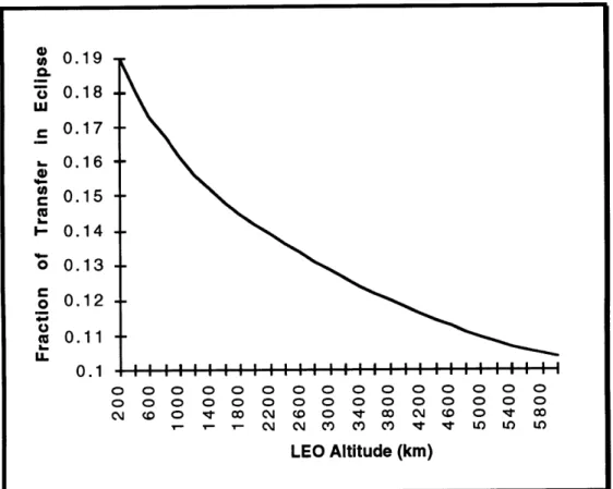
Combining 2.2.4 separately with both 2.2.2 and 2.2.3 yields the accumulated eclipse time and total time for a given change in altitude. These equations can then be integrated numerically over the entire transfer, and the overall eclipse fraction determined. This was done for various LEO altitudes, and the results are given in Figure 2.2.3.

(21)

( 0.19 " 0.18 r 0.17 - 0.16 o 0.15 -- 0.14 o 0.13-0.1 - u-0.1 0 o 00000000000000_{00000000000000} 00 CO C0 c O A t O Cu ( 0 O -0 044 C0 C C ) 0 U) 0

LEO Altitude (kin)

Figure 2.2.3: Fraction of Eclipse Time to Total Transfer Time

From this graph, the burn time (which determines propellant usage) can be related to the transfer time for a given LEO altitude. The burn time for any orbit considered in this analysis will then be approximately 81-90% of the transfer time. Although a constant circumferential thrust was considered for this development, the method of averaging values over an orbit allows the result to extend to arbitrary thrust histories.

2.3 Total Velocity Change (Transfer Energy)

Although a low thrust transfer cannot generally be examined analytically, simplifying assumptions can be made to achieve approximate results. Under the

assumption of low accelerations, where the semimajor axis does not change significantly over one revolution, equations 2.1.2a-d can be applied to the transfer. This allows for the development of a representative AV for the transfer, and subsequent use of the rocket equation to determine propellant usage.

(22)

2.3.1 Orbit Raising

For now, the assumption of constant circumferential thrust and no eclipsing will be considered. With ao constant over a given orbit, equation 2.1.2c integrates (dropping the

brackets) to:

--dR _

= 2 a0 (2.3.1)

dt

Separating variables this can now be integrated over the entire transfer to obtain:

RL R = adt (2.3.2)

R'LEO RGEO

where the transfer time (tt) has been replaced with the burn time (tb) because the

acceleration is zero during eclipse. The right hand side of this equation is easily

identified as the total velocity change (AV) required for the transfer. This gives as a first

approximation a velocity change of 4700 m/s for the LEO to GEO transfer.

This calculation does not take into consideration the change in inclination that must occur if the spacecraft is launched away from the equator. Throughout the calculations, it will be assumed that the launch site is at 28.50 latitude. Although the minimum propellant transfer could be obtained by waiting until the spacecraft has

reached GEO, where the inclination change is most effective, this also provides for the longest transfer time. It would appear that a trade-off, based on cost, would exist which could optimize the altitude at which the inclination change should initiate. For the purpose of this analysis, however, it will be assumed that from a cost standpoint the transfer time is a more valuable commodity than the propellant savings and both will be performed simultaneously. Should the analysis yield marginal results, this is an area that may warrant further consideration.

2.3.2 Inclination Change[5]

To perform a combined orbit raising and inclination change it is required that the thrust be given both circumferential and normal components to the orbit. Examination of equation 2.1.2d shows that the cosine dependence implies the most effective inclination

(23)

change corresponds to thrusting near the line of nodes (near 0* and 1800). This is

reasonable, since the line of nodes is precisely where an impulsive burn would be done to initiate an inclination change. Because an impulsive burn is not possible, an out-of-plane thrust profile must be developed, so that the cumulative effect of the low thrust can be realized efficiently. Although not necessarily optimal, the assumption of a sinusoidal varying thrust profile will allow for continuing to analyze the system analytically, and provide results accurate enough for the purpose of the present analysis.

The out-of-plane thrust (ah) will be given as adsinaocose, where the scaling factor sinto is used for reasons that will become clear. Inserting this thrust profile into equation 2.1.2d and integrating over a single orbit yields:

di ad sin R

- = M (2.3.3)

dt 2

In a similar manner, inserting what remains of the thrust vector into equation 2.1.2c as the circumferential thrust (ae) results in:

dR 4 R3

dR E(sin) o) (2.3.4)

dt n

where the factor E(sinoxo) represents the complete elliptic integral of the second kind. This factor is just a constant for a given value of ao, and as before this equation may be integrated to obtain:

SE(sinao) addt (2.3.5)

RLEO RGEOf

Again, the integral on the right is readily identified with the AV of the transfer, and it can be seen that the result is identical to that found before, but scaled up by the reciprocal of the factor preceding the integral. This factor is necessarily less than unity.

The value of

co

that will properly synchronize the inclination change with the

orbit raising is found by taking the ratio of equations 2.3.3 and 2.3.4 to get:

di _ n sin _(2.3.6)

(24)

Once again separating the variables and integrating over the entire transfer gives:

Ai = t sino n(RGEo (2.3.7)

8 E(sin ao) RLEO )

whereby given a LEO altitude, the value of co can be determined for the transfer. For a

representative 200 km LEO altitude, a, = 600, and the total AV=6000 m/s.

2.3.3 LEO Drag

A consequence of having such low thrust and large solar panels is that drag effects in LEO can become a sizable percentage of the thrust. The resulting transfer is affected in two ways. First, the acceleration is reduced which increases the overall transfer time,

and second, the energy required for the transfer (AV) is increased since deceleration due to drag must be overcome. It was decided for this analysis to set the lower limit of LEO altitude to 200 km, where the thrust to drag ratio is so large that the drag effects can be ignored.

2.3.4 Eclipse

From section 2.2, the effect of eclipsing was found to diminish the effectiveness of the thrusting for a given orbit. The amount of the reduction is altitude dependent, and given in figure 2.2.2. Because this reduction affects all the components of the thrusting equally (turning them off for periods) and the relation of the averaged circumferential to normal thrust is a fixed ratio over the entire transfer, this reduction can be incorporated by scaling the overall AV by a constant factor that is only dependent on the LEO altitude. This factor is determined by numerically averaging this reduction over the transfer in a manner similar to how the eclipse time was determined in section 2.2. For the 200 km LEO orbit, this factor will increase the AV by about 20%, yielding a final value of 7200 m/s for the transfer.

2.3.5 Power Loss

An important factor that comes into play when analyzing space solar arrays is the power loss caused by radiation damage to the cells. This places material dependencies

(25)

back into the orbital equations. To avoid this, a method similar to that used for eclipsing was implemented, through which a specific power reduction coefficient was determined. Even for different transfer rates, the same proportionate times are spent at each radial distance where the electron and ion fluences are known. For a given array material, the rate at which these fluences effect the material have been found experimentally, and by weighting the loss rate by the fractional time spent at a given radial distance the overall loss factor can be determined.

2.4 Launch Systems

There are a number of launch vehicles available, not only in the United States, but other countries as well. The U.S. alone can launch payloads into LEO ranging from as

little as 450 kg to as much as 24,000 kg. The larger launch vehicles, through the use of a

second stage can also transport payloads to GEO ranging from 900 -5200 kg. The cost

to use a given launch vehicle does not vary a great deal with the mass launched, because there is no way to use a fraction of the resources required to launch less than the

maximum capacity of the vehicle. The variation in cost comes from the decision of which launch vehicle to use for a particular mission.

Because of the size and weight of the solar arrays required for the system being considered, it is likely that the larger vehicles, which are already capable of delivering payloads to GEO, will provide the best basis for improved performance. This is because the array mass will represent a small fraction of the total mass of the system. It is also of great interest, however, to see if a smaller scale second stage launched from a vehicle such as a Pegasus would enable placing a payload into GEO where before it was not possible. Not only would this allow small payloads to be placed into GEO at a significant cost savings, but it would provide the opportunity to develop a smaller scale version of the transfer vehicle to prove the technology. Table 2.4.1 lists the launch vehicles being considered, along with launch costs and payloads to both LEO and GEO.

(26)

Launch Vehicle Payld to LEO (kg) Payld to GEO(kg) Cost (M$)* Pegasus 356 --- 17 Delta 7920 5000 910 51-57 Atlas II 6600 570 80-91 Atlas IIAS 8800 1050 125-137 Titan IV 15000 2500 171-258 Space Shuttle 24000 2360 280

Table 2.4.1: Launch System Payloads and Costs * Cost inflated from 1990 values using factors from the Office of the Secretary of Defense

The shuttle is not considered as a launch alternative for the simple delivery mission because the human observation made available by the shuttle is not necessary. Its use will be for missions requiring system retrieval from LEO.

2.5 The Rocket Equation

Having developed the AV for the transfer, it is now possible to apply the rocket equation to evaluate propellant usage and transfer time. The rocket equation is given in one form by:

AV = _{gIlSP In} _f (2.5.1)

where the initial mass is given specifically by:

Mo = MA + MT + Mp(l+ fT)+ MF + ML + Ms + MCNST (2.5.2)

and the final mass is just the initial mass with the propellant mass subtracted. These terms are not all independent, and can be tied together in the following manner. The power used by the spacecraft when not in eclipse is composed primarily of the power used by the thruster (PT), but also includes the power used by the other systems (Po). The power used by the thruster comes from the power realized in the exhaust stream,

(27)

d

1

)1 i(ISPg)2 _(2.5.3)

PT = _I2mv2 ₌ _(2.5.3)

dt 2 TIT 211T

Although the power used by the other systems will vary at different points during the orbit, the array must be sized to allow for all of the systems to be drawing power at the same time. For this reason, Po can be taken as constant, where its value will be the maximum expected draw from all of the systems. The solar array mass can be related to the power requirements through the specific power:

MA =(PT + Po) (2.5.4)

and the propellant mass can be related to the mass flow rate by the equation:

Mp = rthzb (2.5.5)

where tb is the burn time, and equals the difference between total transfer time and

eclipse time. At this point, the independent mission design variables have been reduced to:

1) Launch vehicle

2) Thruster type (Isp, rh , rT) 3) Array type (a)

4) LEO altitude

The first three are discrete, and are not "varied" as such, but rather specific cases will be chosen for examination. The true variables become Isp, rh, and the LEO altitude. These are varied to determine the optimal values for a given system configuration.

3. Mission Scenarios

3.1 Simple Delivery

The simple delivery scheme is most like the current method of payload insertion. The transfer vehicle has a fixed design specification and acts as an independent second stage vehicle. It possesses all of the subsystems necessary to perform the transfer and leave the payload inactive until delivery. It should also be launchable on any of the

(28)

expendable vehicles (or at least a subset) that are currently used in the same manner with a chemical second stage. The advantage of such a system is that the satellite

manufacturer need only meet one requirement beyond what is normally specified for the chemical second stages. This extra requirement is the shielding needed to protect

sensitive parts of the payload during the slow transfer.

The cost function for this system includes operational costs for all of the equipment during the transfer, as well as its full purchase cost because it will be used

only once. Using the cost parameters defined in section one, the cost function takes the following form:

C =CT +CA +CP +CF +CS +CL +CMC +CCNST (3.1.1)

where CCNST has been introduced to represent all of the costs that will remain constant during the analysis.

3.2 Integrated Delivery

Although the simple delivery allows for more freedom in the satellite design, the combination of transfer vehicle and satellite has many redundant systems that could be eliminated for a reduction in cost. Among these are the power supply, communications, GN&C, and much of the structural elements. The transfer vehicle would consist of all of the systems that would normally be present, but there would be mounting surfaces for the equipment that would normally be located in a separate satellite. The immediate

advantage of this is the reduced cost of the original satellite. The transfer system would represent a satellite bus that could be modified to perform any necessary tasks. An

additional savings comes in reducing the transfer time dependent costs. Since the original amount borrowed or otherwise not invested is reduced, the interest accrued over the time of the transfer is also reduced. Further, the power requirement of the transfer

stage will be far greater than what is commonly needed for communications systems, so that the available power to the satellite will likely be greater. There may be implications of this higher power availability that were previously ignored (such as smaller antennae) because the justification of such large arrays was not there.

One possible drawback that goes along with the increased power level in GEO is the increased spacecraft moment of inertia due to the large arrays. This presents a

(29)

greater strain on attitude controlling systems and requires more propellant to be reserved for station keeping. On the other hand, the increased power level will also allow for the use of higher power electric thrusters that will use less propellant. This tradeoff is very specific to the spacecraft in question, and will be left for future analysis. In cases where the total power of the arrays will be utilized there is really no problem, but for cases when less power is required it may be possible to expel unnecessary outer segments of the arrays to reduce the moment of inertia.

With these modifications, the cost function for the integrated delivery mission has the same form as for the simple delivery, but the mission control cost is modified by the reduced initial cost of the system, and the constant term is modified reflecting the systems which will be left out to avoid redundancy. The resulting function is as follows:

C =CT +CA +CP +CF +Cs +CL +CMC + CNST (3.2.1)

3.3 Multiple Payload Delivery

In anticipation of larger payload fractions resulting from reduced propellant requirements, the possibility arises of delivering more than one payload to GEO for each

launch. The maneuverability of this system would allow for it to deliver a payload to its proper position in GEO, and then lower its orbit slightly, allowing it to speed up and re-synchronize at another point in the orbit. Inclination changes would no longer be necessary as the SEOTV "hops" from one position to the next in the orbit, and from equation 2.3.1 it is seen that orbit raising/lowering at these high altitudes is very efficient.

Depending on the size of the payloads, it may be possible to deliver two or more payloads to GEO with each launch. Modifications to the cost function would include altering the mission control costs for the added maneuvering requirements and transfer time, and multiplying the whole thing by the fraction of total payload that belongs to a given user. The resulting function is then:

C = (CT +CA +CP +CF +CS + C + CCNST) (3.3.1)

(30)

3.4 Deliver and Return

This option will utilize an aspect of this system that is not readily available to chemically based systems. Because of the high specific impulse of the thrusters, the propellant usage is greatly reduced. One possibility is to carry enough propellant on board to allow the vehicle to spiral back from GEO to LEO, where it could be picked up by a shuttle flight and returned to the ground for reuse. The transfer vehicle would have a design similar to the simple delivery in that it is a separate unit from the delivered payload, but there is still a significant modification of the cost function. On the down side, a second launch cost is incurred to allow for the recovery of the spacecraft. This will, however, be at a reduced cost because the recovery would not likely be the primary job of the shuttle during its mission. On the positive side, the spacecraft does not need to be purchased as such, but rather rented. The propellant cost and any radiation repair will still be present, but the purchase cost of the spacecraft may be spread out among all of the users over its lifetime.

Given these considerations, the cost function is modified to achieve the following form:

C = D(CT + CA +CF + CCNST) + C +(CL +CMC + )1 +(CL +CM + CP )2 (3.4.1)

where D represents the fraction of the cost that a given user would contribute to pay for the spacecraft, and the grouped terms with subscripts refer to those quantities that will be present separately for the raising (1) and return (2) legs of the trip. It is evident that unless the third bracketed quantity is shown to be less than (l-D) times the first bracketed quantity, it is impossible for this scenario to outperform simple deliveries. Even then, the increased propellant mass and transfer time required to raise the additional return propellant could result in higher net cost than a simple transfer. These issues will be

addressed more fully later.

4. State of the Art

The following sections describe the state-of-the-art in equipment that will be considered in the analysis. In section one the parameters that dictate performance were

(31)

determined, and they will now be given values or ranges of values that are used in the analysis.

4.1 Solar Cells

There are many types of semiconducting materials that may be used to convert solar energy into electricity. The most commonly used today is silicon. There have been great advances in manufacturing made in the area of ground-based solar array

technology, and silicon solar cells can be made rather cheaply. Unfortunately, the

longevity, reliability, and performance requirements demanded of space-based solar cells brings with it a price tag that is still quite high. This is due in part to a limited demand for space photovoltaics.

4.1.1 General Information

In evaluating solar cell performance, a typical parameter used is the cell

efficiency. This number represents the fraction of power that the cell will provide over the available power radiated into a given area of the cell. The available power being radiated is a function of the distance from the sun, and in the Earth's orbit is about 1351

W/m2 [6]. The efficiency of a solar cell is related to the wavelengths of light that the cell

will absorb, and the power density radiated from the sun at those wavelengths. Because the light radiated from the sun is attenuated as it scatters through the Earth's atmosphere, a given cell's efficiency will differ whether it is used on the ground or in space. For this reason, the efficiency is always given with an indication of the air mass that the light passes through before reaching the cell. In space, therefore, the value is given assuming zero air mass (AMO), where on Earth it is referred to as Air Mass 1.5 (AM1.5). There is in general a drop in efficiency of around 15-20% [7] in going from AM1.5 to AMO.

Although efficiency is a convenient and informative parameter to compare cell performance, it is not the most pertinent information for space-based solar arrays. A more important parameter for use there is the mass specific power of the cell, usually given in units of W/kg. This number indicates the important trade-off between power availability, and mass penalty of the power system. For example, if a silicon based solar array is quoted with having 15% efficiency, and a second array made of material X is 30% efficient, but 1/3 of the specific power of silicon, the silicon array will still be better. This is because for a given power level, the silicon array will only weigh 1/3 of the array made from material X, even though it will need twice the surface area. The performance

(32)

of various cells is usually given in terms of efficiency because their use is predominantly ground-based where area rather than weight is the driving factor.

Another important attribute of solar cells for use in space is their resistance to radiation. In particular, solar arrays in orbit are subjected to high energy protons and electrons which upon impacting areas of the array will alter the ordered semiconductor lattice. The irregularities introduced will reduce the freedom of the electrons to move about within the lattice, and reduce the efficiency of the cell. To account for the loss of power over the lifetime of the array, it must be oversized so that the end of life (EOL) power supplied is sufficient to operate all of the systems. Cells which are more resistant to radiation reduce the amount of extra size the array must have in order to provide sufficient EOL power.

For a given cell material, a trade-off can be made between specific power and radiation resistance through the use of a cover glass. As the thickness of the cover glass is increased, the high energy particles will be decelerated through more collisions before reaching the semiconducting material, and will not cause as much damage. By the same token, the cover glass represents an added mass to the system without adding any extra power, so that the specific power of the system goes down. Modifying the geometry of the cover glass so that it resembles a grid of tiny lenses has the effect of increasing the intensity of the light falling on the lattice. The resulting cell is called a concentrator (see Figure 4.1.1), and its benefit is two-fold. First, the efficiency of most cells increases with the intensity of the light falling on them. Second, since the light is focused on smaller areas, less of the expensive semiconducting material is required to construct the cell. The down side of such a configuration is that by introducing the lenses, there is a greater need for precision pointing of the solar array toward the sun.

(33)

Figure 4.1.1: Solar Cell with Concentrator Cover Glass

4.1.2 Current Values

For the purpose of this study, three cell structures will be considered. The first is the state of the art in silicon cell technology, and will be employed on the space station. The second is constructed of Gallium Arsenide (GaAs), which has been shown to have the highest specific power to date as well as improved radiation resistance. The third is constructed from Indium Phosphide (InP, )which although it does not have as high a specific power as GaAs exhibits superior radiation tolerance. Table 4.1.1 summarizes the important parameters of each cell type.

Cell Type Efficiency (%) Spc. Pow. (W/kg) Cost (K$/W)[7]

Silicon 15 113 1

Gallium Arsenide 19 131 33

Indium Phosphide 18 126 66

Table 4.1.1: Comparison of Cell Types Considered[8]

The cells were similarly constructed to be 2 mils thick with a 10 mil cover glass. It is possible that the performance of these cells could be improved by including

concentrators or by stacking cells that are sensitive to different spectral ranges. By comparing these basic cells, however, it is possible to see how their different qualities

(34)

affect the optimization of the problem, and from that can be extracted what modifications of these cell types would be most beneficial.

As stated above, one of the important characteristics of these cells is their

resistance to radiation. This particular aspect will have more or less relevance depending on the reusability of the spacecraft. In the event that the cell with the highest radiation resistance was also the most efficient, had the highest specific power, and cost the least, there would be no question -- this, however, is not the case. Figure 4.1.2 shows the effect of long exposure time at 11000 km altitude and 00 inclination. This corresponds to radiation bombardment that would be among the most severe over the time of the transfer.

It can be seen from Figure 4.1.2 that although GaAs has a greater specific power at BOL it drops more rapidly than InP and after about 6 months is actually lower in value. The actual degradation during a transfer will not be this great because the spacecraft will pass into and then back out of this region of high radiation. For short transfer times without reusability, the lesser cost of GaAs makes it a likely candidate over InP. For long or multiple trips, the InP may begin to look cost effective, but neither is likely to be competitive with Si.

140 •- --- Si 120 M. 100 --- GaAs InP 80 "6 60 40 - - - - -20 0 1.5 3.5 5.5 7.5 9.5 Years in Orbi"

(35)

4.1.3 Power Conditioning

The problem of power conditioning was addressed briefly in section 1.2 in the discussion of the thrusters. Power conditioning is necessary to match the power output of the solar arrays to the various subsystems of the spacecraft. It is also necessary for the protection of the arrays themselves, by ensuring during the transitional periods in and out of eclipse that the power generating areas of the arrays are not back-feeding the areas in shadow.

One way of dealing with the power conditioning is to use a main system at the output of the arrays that distributes power over the entire spacecraft. The system usually provides several levels of redundancy, and the added mass is factored into the specific power of the power system, reducing it significantly. The mass of the PCU does not scale directly with the power level, and at higher power levels the effect is not as significant as at lower ones.

Another way of handling power conditioning is to allow for each subsystem to regulate its own power. Usually this creates a lot of redundant hardware mass, because the power requirements of the various subsystems are all within the same range. In the present example, however, it will be seen that the power usage of the thrusters constitutes

all but a small percentage of the power available. Since the PCU mass is already counted in the propulsion system mass, it will be associated with it rather than with the power system. The PCU mass associated with the rest of the subsystems is not significant as compared to the power levels of the solar arrays, and so the values of the array specific power are not much less than without power conditioning.

4.2 Thrusters

For the present analysis, three types of thrusters will be considered. These are: 1) Arc jets

2) Stationary Plasma (Hall Effect) 3) Magnetoplasmadynamic (MPD)

(36)

The performance of Ion engines will actually be implicitly included in the analysis of MPD thrusters, because their range of specific impulse and efficiency are very close.

4.2.1 Arc jets

The arc jet is the representative member of the electrothermal family of thrusters. Current supplied from the power source is used to maintain a steady arc through which the propellant passes on its way to the nozzle. The thermal energy from the arc is transferred to the propellant and increases its enthalpy above what could be obtained using chemical combustion. The propellant is then expanded in the usual way, allowing the stored energy of the fluid to be converted into kinetic energy. There is much

experimental data on arc jet thrusters, and each experimental setup produces slightly different performance data for them. The following table summarizes the values that were used for this study.

Thrust (N) 1.32- 1.98 Isp (s) 700- 820 Efficiency (Thrust) 28 - 32 Efficiency (PCU) 90- 92 System Mass (kg) 39.0 Thruster (kg) 5.0 PCU (kg) 34.0 Cost (K$) 100

Table 4.2.1: SOA High Power Ammonia Arc jet[1]

4.2.2 Hall Thrusters

The Hall Effect Thruster, also known as the stationary plasma thruster (SPT), is a form of electromagnetic propulsion. The thruster consists of two concentric cylinders, between which the propellant flows. The propellant is fed through the back wall, and ionized by electrons that are held in orbit by a radial magnetic field. The ions are then accelerated over the length of the cylinders by an electric potential, in much the same way that ion thrusters operate. Because there is a balance of electric charges in the region

where the ions are accelerated, however, the Hall Thruster is not subject to the same space-charge limitations of the ion engine. There is ever increasing data on a specific thruster which has been developed in recent years by the Russians. The data for this thruster, the SPT-100, was used in this analysis and is summarized in table 4.2.2 on the following page.

(37)

Thrust (N) 0.06 - 0.08 Isp (s) 1500- 3000 Efficiency (Thrust) .50- .70 Efficiency (PCU) .95 System Mass (kg) 8.0 Thruster (kg) 4.0 PCU (kg) 4.0 Cost (K$) 500

Table 4.2.2: Hall Thruster (Stationary Plasma Thruster)[9]

4.2.3 MPD Thrusters

The MPD Thruster has a similar geometry to that of the Hall thruster. It consists of two concentric cylinders, which in this case represent an anode and cathode. A plasma located between the plates is forced to begin separating radially under the influence of the electric potential. The electric current for both ions and electrons is radially toward the cathode (negatively charged particles carry current opposite to their direction of travel). As the charged particles move radially, the current density changes due to the cylindrical geometry, which induces a magnetic field in the azimuthal direction. A Lorentz force is

developed axially from the j x B interaction of the current with its own induced magnetic

field which accelerates the particles out of the thruster.

These thrusters are still in their experimental phase, but with the capacity to operate at very large power levels they could someday be the ideal device for lifting heavy payloads to higher orbits. Table 4.2.3 summarizes their performance.

Thrust (N) 17.6 - 110 Isp (s) 2000- 5000 Efficiency (Thrust) .35- .55 Efficiency (PCU) .98 System Mass (kg) 150 Thruster (kg) 34 PCU (kg) 116 Cost (K$) 500

(38)

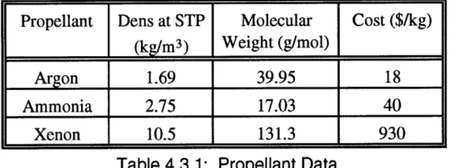
4.3 Propellant / Tankage

The cost of propellant and tankage are considered together because they both scale with the propellant mass. The tankage fraction, as found from equation 1.3.3, is seen to depend on both the type of propellant and material used for the tank. Similarly, these factors determine how the tankage fraction is to be modified in equation 1.3.4 to calculate the combined propellant/tank cost. Some representative values are given below.

Propellant Dens at STP Molecular Cost ($/kg)

(kg/m3) Weight (g/mol)

Argon 1.69 39.95 18

Ammonia 2.75 17.03 40

Xenon 10.5 131.3 930

Table 4.3.1: Propellant Data

Material Density Ultimate Cost ($/kg)

(kg/m3) Strength (MPa)

Aluminum 2800 523 10

Graph/Epox 1490 1337 78

Kevlar 1380 1378 63

Table 4.3.2: Tank Data

4.4 Guidance, Navigation and Control

Because solar arrays are being used as the power source, they must be kept facing at the sun at all times. This represents a nearly inertial reference frame with a rotation rate of only a degree per day. Rotation this slow cannot be used for stabilization, and because of the extraterrestrial pointing, neither can gravity gradients or magnetic torques. The only alternative is a three-axis stabilized spacecraft. Normally, reaction wheels would be used to absorb torques on the system, however due to the large moment of inertia with the large solar arrays, control moment gyros and even hot or cold gas

(39)

thrusters may need to be employed. Table 4.4.1 summarizes performance of some common actuators.

Actuator Performance Mass (kg) Power (W)

Range Thrusters

Hot gas .5 to 9000 N Variable N/A

Cold gas <5 N Reaction & 0.01 to 1 Nm 2 to 20 10 to 110 Momentum wheels Control 25 to 500 Nm >40 90 to 150 Moment Gyros (CMG)

Table 4.4.1: Typical GN&C Actuators[6]

To maintain the sun pointing vector for the solar arrays, it is necessary to determine the direction of the sun at all times. This is accomplished through the use of sun sensors. Alone, however, they can offer only a single vector in space, and must be accompanied by other devices for complete attitude information. As mentioned earlier,

one of the recurring problems with low thrust transfer is repeated solar occultation when the Earth passes between the spacecraft and the sun. At these times, it will be necessary to employ some alternative attitude sensor also. One possibility is through the use of horizon sensors, but because the Earth's position will be changing relative to the attitude

of the spacecraft, a second inertially referenced sensor -- a star sensor -- would be better

suited. The combination of sun and star sensors will then be sufficient to determine the attitude of the spacecraft at all times. Table 4.4.2 gives information on some of the available sensing equipment.

(40)

Sensor Performance Mass (kg) Power (W) Range

Inertial Gyro drift rate

measurement 0.003°/hr to 3 to 25 10 to 100 unit 1 °/hr accel. (IMU) Sun sensors 0.005' to 30 of 0.5 to 2 0 to 3 accuracy Horizon sensors 0.1" to 1l of Scanner accuracy 2 to 5 5 to 10 Fixed head 2.5 to 3.5 0.3 to 5

Star sensors 1 arc sec to 1

(scanners & arc min of 3 to 7 5 to 20

mappers accuracy

Table 4.4.2: Typical GN&C Sensors[6]

4.5 Communications

As was stated in section 1.5, the communications system is not the focus of the

study and one is simply chosen that will suffice. Table 4.5.1 gives the parameters for a typical S-Band communication system compatible with the Tracking and Data Relay

Satellite System (TDRSS).

Component Mass (kg) Power (W) Dimensions (cm)

Transponder 13.74 14 x 33 x 14 - Receiver 17.5 - Transmitter 45.0 Filter / switch 2.0 0.0 15 x 30 x 6 diplexers / etc. Antennas - Hemis 0.8 0.0 9.5 dia x 13 - Parabola 9.2 0.0 150 dia x 70 - Turnstile 2.3 0.0 10 dia x 15

- Coax Cables 0.5 0.0 1.2 dia x 150

Total 28.54 62.5