Mechanism of shock unsteadiness in separated shock/boundary-layer interactions

HAL Id: hal-01455109

https://hal.archives-ouvertes.fr/hal-01455109

Submitted on 3 Feb 2017

HAL is a multi-disciplinary open access

archive for the deposit and dissemination of

sci-entific research documents, whether they are

pub-lished or not. The documents may come from

teaching and research institutions in France or

abroad, or from public or private research centers.

L’archive ouverte pluridisciplinaire HAL, est

destinée au dépôt et à la diffusion de documents

scientifiques de niveau recherche, publiés ou non,

émanant des établissements d’enseignement et de

recherche français ou étrangers, des laboratoires

publics ou privés.

Lionel Agostini, Lionel Larchevêque, Pierre Dupont

To cite this version:

Lionel Agostini, Lionel Larchevêque, Pierre Dupont.

Mechanism of shock unsteadiness in

sepa-rated shock/boundary-layer interactions. Physics of Fluids, American Institute of Physics, 2015,

27, pp.126103 - 126103. �10.1063/1.4937350�. �hal-01455109�

SEPARATED SHOCK/BOUNDARY-LAYER

INTERACTIONS

L. Agostini,1_{L. Larchevˆeque,}1 _{and P. Dupont}1

Aix-Marseille Universit´e, CNRS, IUSTI UMR 7343, 13013, Marseille, France

(Dated: 8 December 2015)

An LES-based study is presented and focuses on different unsteadiness-source fea-tures in a Mach 2.3 shock reflection with separation. Sources of unsteadiness are localized and the path taken by disturbance as it spreads out to the whole field is defined. It is shown that phenomena arising inside the recirculation bubble govern the whole interaction, at both low and intermediate frequencies. Indeed the shock motion appears to mirror phenomena found in the separated zone. Moreover, fea-tures of separated–flow unsteadiness bear some resemblance to those occurring in incompressible flows. An equivalent inviscid scheme of the unsteady interaction is established in order to describe the whole shock-system unsteadiness at low and intermediate frequencies and the downstream unsteady-pressure field.

Keywords: separated flow, shockwave/boundary-layer interaction, Large-Eddy Simulation

I. INTRODUCTION

Shock wave/boundary layer interactions (SWBLIs) are ubiquitous in high speed aero-nautical applications. Whatever the flow configuration under consideration (compressions ramps, shock reflections, blunt-fin or over-expanded nozzles), separation-shock displacement occurs at low frequencies. Fully–separated interactions have been widely studied in the past by means of scientific experiments1–7_{. More recently, additional information has been} ob-tained from Direct Numerical Simulations8 (DNS) or Large-Eddy Simulations9,10 (LES). Nevertheless the origin of low-frequency shock displacements is not yet clearly established. In high Reynolds cases, upstream perturbations have been shown to influence separation– shock motions6,11,12. However these experiments are considered to be nearly attached/incipient– separation configurations for which no reverse flow could be observed from Particle Image Velocimetry (PIV) measurements in a time–average sense.

Comparisons between two incipient-separation cases, respectively at low and high Reynolds number13,14 _{confirm that the separation-shock displacement is correlated with} the upstream–boundary–layer unsteadiness and also with unsteadinesses located in the interaction region developing downstream from the separation shock. In separated cases, for which a well-defined mean-recirculation region is observed, recent results obtained for low Reynolds number SWBLI5,8,15 have shown that low-frequency shock unsteadiness has to be related to the downstream part of the separated flows.

Several models derived from experimental data and numerical simulations were intro-duced in order to define the sources of low-frequency unsteadiness, see Morganet al.10 for a recent review. Touber and Sandham16 _{and Priebe and Martin}17 _{suggest that they have to} be related to an instability of the separation bubble, induced by a stationary global mode, which leads to self-sustained oscillations of the interaction region and to specific time evo-lution of the skin friction coefficient. Nevertheless, different results are proposed by Touber and Sandham18: using several hypotheses based on data from a LES of an 8◦shock reflec-tion, these authors derived an equivalent low-pass filter system, as previously suggested by Plotkin19_{and Poggie and Smits}20_.

On the other hand, Piponniau et al.21 suggest that the observed low-frequency unsteadi-ness of the separated bubble is related to mass entrainment across the mixing layer which

gests that there is a direct link between the Kelvin–Helmholtz–like convective structures in the mixing layer and low-frequency unsteadiness in the separated region. The convective structures are associated with what will hereafter be referred to as “medium frequencies” since they are one order of magnitude higher than the low frequencies related to the bubble breathing and also one order of magnitude lower than the energetic eddies in the upstream boundary layer. The development of these structures has been identified from unsteady wall-pressure measurements5 and from PIV data15. The low-frequency breathing of the separation bubble and shock displacement were found to be linked, and there is some evi-dence of similarities between the separated regions in SWBLIs and incompressible separated flows , although significant influence from compressibility effects are expected in the mixing layer. The model was able to give some relevant scaling for low-frequency shock unsteadi-ness in various SWBLI configurations, but detailed descriptions of the process were not addressed.

Moreover, several experimental results obtained in various SWBLIs are not yet clearly explained by these different models. For example, it has been known for decades that specific phase relationships are observed from unsteady wall-pressure measurements1,2,5_{. It} has also been shown that, whatever the geometry (compression corner or shock reflection) and Mach number (1.5 < M < 5), strong correlation at low frequency occurs between wall pressure fluctuations created by the shock unsteadiness and those downstream from the shock. The initial region of the interaction exhibits in–phase pressure fluctuations, while the region near the reattachment point presents anti–phase pressure signals. These two regions are separated by a zone of null correlation whose origin is not yet well established. This paper will take advantage of recent LES of the shock reflection based on the config-uration studied experimentally at the IUSTI laboratory. The simulations are obtained over a long time with respect to the low-frequency unsteadiness (typically sampling more than 150 cycles) so as to generalize experimental observations at the wall to the whole flow field. The objectives are:

• to localize the source of interaction unsteadiness at low and medium frequencies, • to describe the spatial links leading to the observed pressure fluctuation levels in the

field,

• to give a simple inviscid scheme, involving the subsonic near-wall region, the super-sonic external flow with the shock system, and the downstream region.

The paper is organized as follows. Section II recalls the numerical method and flow parameters and presents validation versus experiments. In section III, the spatial links between the separated bubble and the external flow are identified. In Section IV, the near-wall pressure unsteadiness will be investigated and compared to incompressible separated flows. This analysis will be extended to the supersonic region of the interaction in section V. An equivalent simple inviscid model, summarizing all the observations and results, is pro-posed in section VI. Lastly, properties shared by both incompressible and compressible separations will be discussed and the inviscid model will be extended to medium-frequency unsteadiness in section VII.

II. FLOW PARAMETERS AND COMPUTATIONAL DETAILS

A Mach=2.3 shock reflection on a flat plate is considered. Experiments are set up in IUSTI’s supersonic-wind tunnel and LES of the flow is achieved at the same Reynolds num-ber as the experiments, namely Reδ2 = 5000, where δ2stands for the momentum thickness of the upstream boundary layer. This experimental set-up and its main results have been described in previous workss5,15,21–24. The upstream flow parameters are given in table I. An interaction with flow deviation of 9.5◦, corresponding to a noticeable separation, is con-sidered in the present work. A schlieren picture of the interaction is given in figure 1(a) and

TABLE I. Flow conditions of the interaction M Reδ2 U∞[ms −1 ] δ0[mm] δ2[mm] P0[P a] Tt[K] Flow Deviation[◦] 2.3 5.1 × 103 _{557 11 0.96 0.5 × 10}5 _{293 9.5} (a) 0000000000000000000000000000000000000000000 1111111111111111111111111111111111111111111 X0 XR L point Separated Reattachment point

H

FIG. 1. (a) Schlieren picture of the shock boundary layer interaction carried out in IUSTI’s wind tunnel and (b) sketch of the main features of this interaction.

its main features are highlighted in figure 1(b). Note that sketch 1(b) includes the compres-sion waves located upstream from the expancompres-sion fan, as seen in figure 1(a) and that such compression waves are incompatible with the standard inviscid modeling of a separated in-teraction25. This point will be further discussed in sections III and VI A. The experimental set-up yields some significant three-dimensional organisation of the interaction22, the origin of which has been identified from numerical simulations as being the side wall boundary layer26,27_{. Mean turbulent-velocity fields and time properties of the flow have been derived} from PIV15,21_{, hot–wire, and unsteady wall–pressure measurements}5,23_{. For the} experi-ments and the LES, low-frequency unsteadiness of the separation shock were observed and associated with a characteristic non-dimensional frequency, or Strouhal number, such as:

SL= f L U1

' 0.03 (1)

where f is the frequency of pressure fluctuations at the mean location of the separation– shock foot (defined as the location where the standard deviation of wall pressure fluctuations is highest), L is the interaction length and U1 is the external velocity downstream from the incident shock. The length L is defined as the distance between the mean location of the separation–shock foot, denoted X0, and the extrapolation down to the wall of the incident shock.

The LES results used in this article were designed to achieve long-time integration en-compassing a large number of low-frequency cycles. Consequently the three-dimensional organization of the flow was not taken into account and periodicity conditions were used in the spanwise direction, as in previous LES of similar flows9,28_{. The length and span of the} computational domain are equal to 5.6 L and 1.6 δ0, respectively. The grid resolution has been selected to match the requirements of a wall-resolved LES, with ∆x+_{' 40, ∆z}+_{' 16} and y₁+' 0.9.

Three additional short-time computations were carried out for validation purpose. The span of the computational domain of the first one has been increased up to 11 δ0 while the

computation has been performed for the narrow domain but using a refined grid, with ∆x+_{' 30, ∆z}+_{' 12 and y}+

1 ' 0.8. The last additional computation has been designed to encompass the shock generator and the full height and width of the wind tunned, equal to 15 δ0 and 17 δ0, respectively. No–slip conditions have been enforced on the ceiling and the side walls. The mesh has consequently been adapted so as to resolve the boundary layers developing along these walls with the same grid resolution as the one used in the vicinity of the floor for the long–time LES.

For all these computations, the effect of subgrid scales on resolved ones was taken into account by means of the selective mixed-scale model29_{. Ducros’ sensor}30_{was used to switch} from a centered scheme in the turbulence–dominated region to a Roe dissipative scheme in the shock region, in order that the numerical dissipation will not mask the effect of the subgrid model. An unsteady condition based on a Synthetic Eddy Method31 was set at the inflow boundary, located 11 δ0 upstream from the interaction region, thus resulting in a fully–turbulent boundary layer upstream from the separation. Characteristic–based non–reflecting conditions were used for the upper and outflow boundaries.

Details on the validation process, including comparisons between experimental data and the above–mentioned simulations with standard, refined and enlarged meshes, can be found in Agostini et al.32_{. Specifically, they show that both the spatial and the temporal flow} organizations are accurately reproduced, despite a slight under-estimation of the interaction length found in simulations with respect to experimental results. The difference is of about 15%, regardless of the flow deviation under consideration, and recent works have shown that this difference is probably due to certain side effects in the experiments associated with the finite span of the wind tunnel26_{. Nevertheless, it is shown in Agostini et al.}32 _{that the} space and time flow properties, when normalized by the interaction length, are accurately reproduced.

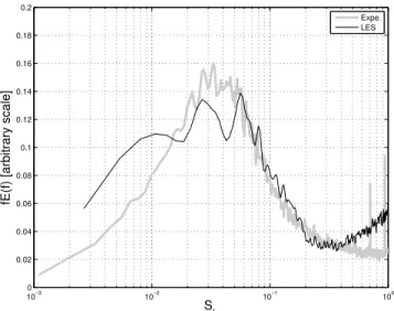
Quite long computations over at least 150 low-frequency cycles allowed the calculation of Power Spectral Densities (PSD) of pressure fluctuations along the interaction which compared very well with the experimental results. The characteristic low–frequency shock motion of a Strouhal number close to 0.03 was obtained for all cases of flow deviations that were tested, including the 9.5◦ case under consideration in this paper. This property is illustrated in figure 2, where the experimental and numerical PSD of the pressure near the mean position at the foot of the separation shock are presented for the 9.5◦flow deviation. The good agreement between confined experiments with side walls and LES with spanwise periodicity, as seen in figure 2, is due to the fact that the mid–span region of the flow is mildly altered by the side–wall separations, with the exception of an increase of the inter-action length. Figure 3 demonstrates that the streamwise development of the interinter-action is very similar between the computation with spanwise periodicity and the computation with side walls, provided that for the latter one only a mid-span region of limited width (2 δ0) is considered and that a rescaling based on the interaction length is performed. Both com-putations result in the expected streamwise evolution from the low–frequency–dominated region near the separation point to the medium–frequency region associated with vortex shedding5, despite the poor statistical convergence of the short–time computation with side walls which last only 10 periods of low–frequency unsteadiness.

Most of the available experimental results concerning space-time SWBLI properties have been derived either from unsteady wall-pressure measurements or from in–field hot–wire measurements1,2,5_{. As recalled in the previous section, several spectral properties (PSD,} phase and coherence relationships) were derived, but mainly limited to wall measurements. Recently, complementary data has been obtained from Dual-PIV measurements13,33 and Linear Stochastic Estimation analysis, applied on simultaneous measurements of unsteady wall-pressure and velocity fields by PIV34_{. These results confirm the low-frequency} cor-relations between the shock motion and the downstream interaction region derived from wall–pressure and hot–wire measurements. In the next sections, space-time resolved com-putations data is used to generalize these results to the whole field in order to identify the different unsteadiness sources and determine how they influence the various flow

re-10−3 10−2 10−1 100 0 0.02 0.04 0.06 0.08 0.1 0.12 0.14 0.16 0.18 0.2 S L

fE(f) [arbitrary scale]

Expe. LES

FIG. 2. PSD of the wall–pressure fluctuations in the vicinity of the mean location of the separation– shock from LES (solid black line) and experiments (solid gray line). The Strouhal number SLis

defined by equation 1.

(a) (b)

FIG. 3. Streamwise evolution of the normalized PSD of the wall-pressure fluctuations for the long–time computation with spanwise periodicity (a) and for the mid–span region of the short– time computation including side walls (b). The normalized streamwise coordinate is defined by equation 2.

gions. Velocity, density and pressure data in wall–normal planes are stored using a 200 kHz sampling rate. This frequency has been checked to ensure that it is sufficient for avoiding any significant aliasing effect for frequencies lower that 20kHz, which allows analysis of the interaction region.

III. SPATIAL LINKS BETWEEN THE SEPARATED BUBBLE AND THE EXTERNAL FLOW The low–frequency unsteadiness of shock displacements generates large pressure varia-tions related to the pressure jump across the shock, denoted ∆ps: it induces a sharp increase in pressure fluctuations such as their RMS values which are equal to half of ∆ps5,24. As

(a)

(b)

FIG. 4. Root Mean Square values of the low–pass filtered (SL < 0.08) pressure p∗LF (a) and

streamwise velocity u∗LF (b) fluctuations. Contour levels of pressure fluctuations have been clipped

to 10% of the maximum value in order to make the plot legible. The streamwise and wall-normal coordinates have been respectively normalized by L and HI (see figure 1(b) and equation 2 for

definitions) and the dashed line denotes the sonic line.

these fluctuations are not directly produced by turbulent phenomena, they will be referred to as intermittent. Similar comments apply for the expansion-wave region, where pressure fluctuations are generated by the oscillations in space of the pressure gradient.

The “intermittent” fluctuations associated with the separation shock and expansion wave are found dominant in figure 4(a), where a map of the RMS values for the low-pass filtered pressure pLF, normalized by the upstream static pressure P0 as p∗LF = pLF/P0, is plotted. The non-dimensional cut-off frequency of the low-pass filter is SLc= 0.08. This frequency range encompasses the low-frequency shock motions, the power spectra of which are centered around SL ' 0.03, see figure 2). The longitudinal dimensionless coordinate X∗ is defined by considering the location of the separation-shock foot and the length of the interaction, defined in figure 1(b), as:

X∗=X − X0

L (2)

The map of the RMS values for the low–pass filtered streamwise velocity u∗_LF, normalized by the upstream velocity U∞, is plotted in figure 4(b). It is seen that the “intermittent” fluctuations induced by the shock motion are milder than their pressure counterparts, a fact that can be explained by noting that the relative velocity jump across the shock is much lower than the relative pressure jump. On the other hand, high levels of u∗_LF are found in the mixing layer and shedding regions. They can mostly be traced back to the breathing of the separated bubble, inducing “intermittent” fluctuations in these regions associated with high value of wall-normal derivatives of the streamwise velocity.

Other regions of the flow display much lower low–frequency pressure fluctuations. In accordance with experimental results5_{, no significant pressure and velocity fluctuations are}

identified for the upstream boundary layer in this frequency range. It must be mentioned that any influence from “super-streaks” on the interaction unsteadiness, as reported in the literature6,12 _{cannot be expected in the present simulation. Indeed, a Synthetic Eddy} Method is used to generate the turbulent boundary condition at the inflow, and the resulting boundary layer develops over a distance of 11δ. This distance is at least three times smaller than the length of these “super-streaks”, equal to about 30δ35_.

Low levels of low-frequency pressure fluctuation are also found unexpectedly in the in-teraction region, in the zone located immediately downstream from the separation shock and above the separated bubble, with RMS values lower than 1.25 × 10−2P0. RMS values increase when moving down into the separation bubble, but still remain weak in that region, labeled B in figure 1(b). Downstream from this region, and up to the reattachment point, in the region of the bubble denoted by C in figure 1(b), the low–frequency fluctuation levels rise smoothly up to a value of about 3.2 × 10−2P0 which is approximatively equal to those found in the outer flow, downstream from the expansion wave.

The strongest low-frequency pressure fluctuations found in the interaction region, apart from the separation-shock and the expansion-fan zones, are located in a narrow band up-stream from the expansion fan and spread out from the impingement of incident shock on the shear layer. Henderson36 has shown that, when a shock impinges a boundary layer, their interaction cannot be restricted to a simple reflection. The incident shock is refracted through the boundary layer and such a refraction results either in reflected compression waves or reflected expansion waves, or in both, depending on the intensity and angle of the incident shock and on features of the upstream boundary layer. The latter process is bound to occur in the interaction studied in this paper since, according to the schlieren picture in figure 1(a), compression waves are found in that narrow region. It will be shown in section V that these unsteady compression waves play a key role in the pressure equilibrium within the interaction.

Study of RMS pressure values at low frequencies shows that the interaction can be split in several parts associated with different levels of RMS pressure. In order to understand this spatial organization, the coherence field between pressure fluctuations and separation-shock displacements has been derived from the time-resolved LES data. The separation-shock motion is estimated, for a given altitude, from the streamwise location of the maxima of the pressure variation induced by the separation shock, detected by computing the pressure gradient in the direction normal to the separation shock32_{. The time evolution of the instantaneous} shock location can then be used to demonstrate the relationship between the shock motion and the interaction region. The coherence function, defined by:

Coh(f ) =_q| dSs,p| c SsScp

(3)

where dSs,pis the cross spectrum between the shock location s and the pressure fluctuations p and cSsand cSpare the PSD of s and p, respectively, highlights the links between the pressure fluctuations and the shock position, independently of any phase between the two signals. Its value ranges from 0 to 1, corresponding to uncorrelated signal and fully correlated signals respectively at the frequency f . The coherence function between unsteady wall pressure induced by the separation–shock displacements and the streamwise distribution of wall-pressure fluctuations has been widely documented from experiments on compression ramps1,2,37 _{and for shock reflections}5,15_{. These works have indicated that wall-pressure} fluctuations in the second part of the separated zone are highly correlated and in anti– phase with pressure fluctuations occurring at the separation-shock foot. These observations have also been confirmed from numerical simulations, DNS38,39 _{as well as LES}40_.

With respect to these studies, use of the shock location in the present experiment, rather than the wall pressure, allows the extraction of a genuine relationship between the shock unsteadiness and the whole interaction. The coherence-coefficient map associated to the Strouhal number of 0.03 is shown in figure 5. The white star marks the reference altitude at which the streamwise location of the shock is estimated. Maximal values are in black

X* Y/H I 0 0.5 1 0 0.5 1 1.5 2 0 0.2 0.4 0.6 0.8 1

FIG. 5. Map of the coherence between the shock displacement at the altitude denoted by a star and the pressure fluctuation p for the typical normalized frequency SL' 0.03 associated with the

low–frequency unsteadiness of the interaction. The dashed line denotes the sonic line.

and minimal values in white. The wall streamwise distribution of the coherence coefficient has the same features as the previous results mentioned above. Nevertheless, using nu-merical simulations, these phase relationships can be extended from the wall to the whole field, and subsequently can identify zones of influence and the links between each of them. For the low frequency range under consideration, no correlation between the separation– shock displacements and the upstream pressure fluctuations is observed, while the largest coherence-coefficient level is found in the region of the separation-shock displacement. The interaction is split into two parts which are strongly correlated, separated by an intermediate region corresponding to a gap of coherence.

Similar results have been obtained from the low–pass–filtered cross–correlations32. It was shown that pressure fluctuations in the second part of the interaction are in phase with the low–frequency shock displacements. They are therefore in anti–phase with the induced pressure variations since, when the shock moves upstream, i.e. for decreasing values of x, pressure at the shock mean position increases whereas when the shock moves in the opposite direction (downstream), the pressure level is reduced. The results presented in this section tend to confirm that separation-shock kinematics at low frequencies is governed by unsteadiness occurring inside the separated zone, as previously found by Agostini et al.32 from analyses based on the theory of characteristics and two-point correlations. Moreover, the fact that the interaction is split into two regions on either side of a coherence gap suggests that two specific dynamics are at work within the bubble. Pressure fluctuation features occurring in the separated zone are described more thoroughly in the next section in order to understand the origin of this coherence gap.

IV. PRESSURE UNSTEADINESS IN THE SUBSONIC DECELERATED REGION A. Wall Pressure fluctuations

In section III, it was shown that the large fluctuations encountered in the region spanned by the motion of the separation shock were intermittent in nature. It is consequently de-sirable to try to remove them in further analyses, since they are associated with purely kinematic effects and are consequently a poor indicator of flow dynamics within the inter-action. The removal can be achieved by considering data in the frame associated with the separation shock, rather than in the laboratory frame.

0 0.5 1 0 0.025 0.05 p * LF X* 0 0.5 1 0 0.5 1 P *

B

C

A

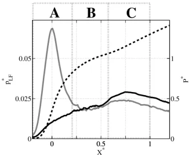
FIG. 6. Streamwise distribution of the RMS values p∗LF of the low–pass filtered wall-pressure; solid

gray line: laboratory frame; solid black line: moving frame associated with the separation-shock frame; dashed line: mean pressure in the laboratory frame. Regions A, B and C are defined in section IV.

RMS values are recast in the moving frame associated with these locations. The resulting streamwise profile is plotted in figure 6 alongside its counterpart computed in the laboratory frame. The dimensionless pressure P∗= (P − P0)/P0 is also reported on the figure. As expected, the large peak of RMS pressure values located in the shock-displacement region, vanishes when the frame associated with the separation shock is considered. This clearly confirms the intermittent nature of these pressure fluctuations, in relation to the large pressure gradient across the separation shock. Downstream, where the pressure gradient is milder, the values obtained in the separation-shock and wind-tunnel frames are close, both increasing up to 3 × 10−2 P0.

Based on these plots, the interaction can be roughly divided into three parts as shown in figure 6:

• In the initial region of the interaction, hereafter referred to as region A and associated with the separation shock, P∗increases very rapidly and a large peak of RMS pressure fluctuations occurs due to low–frequency shock motions found in the laboratory frame. • In the region labeled B, downstream from the separation point with 0.2 < X∗ _< 0.6, the mean pressure increases slowly, without clear plateau, as often reported in largely separated flows, see for instance Delery and Marvin25. These authors however note that, for interactions still resulting in a sizeable separation, the wall pressure distribution displays only an inflection point, as in the present case. Nearly constant RMS pressure fluctuations are also observed in that region.

• Further downstream, in region C defined by 0.6 < X∗

. 1, a nearly constant pressure gradient is observed alongside with a maximum of the RMS pressure fluctuations Low–frequency links between the shock displacement and the wall–pressure fluctuations result in a similar partition of the interaction, as seen in figure 7 where the coherence between the wall-pressure fluctuations and the shock displacements at each altitude is shown for SL= 0.03. Region A is associated with high, nearly constant coherence levels regardless of the shock altitude taken as reference, whereas levels, still high but increasing with the altitude are found in region C. No significant coherence level is found in region C

X* Y/H I 0 0.5 1 1.5 0.5 1 1.5 2 0 0.2 0.4 0.6 0.8 1

A

B

C

FIG. 7. Coherence for SL= 0.03 between the wall-pressure fluctuations at the normalized

stream-wise location X∗and the separation-shock displacement at the normalized altitude Y /HI

.

The accurate matching of regions defined in figures 6 and 7 makes clear that different mechanisms are at play in the interaction and that they influence the low-frequency un-steadiness of the shock. They seem to be associated with three different regions in the interaction. In order to clarify each mechanism, a conditional analysis of the pressure fields, based on separation bubble unsteadiness, is presented in the next section.

B. Conditional analysis based on the bubble unsteadiness

The strong differences found in the pressure RMS values and the coherence maps when moving from region A to C suggest that different behaviors are observed in both the initial and the final part of the interaction. However, as seen in figure 6, large fluctuations in the initial region of the interaction are induced by the kinematics of the separation shock and are therefore irrelevant when analyzing the intrinsic bubble unsteadiness. The separation–shock reference frame is consequently reviewed throughout this section.

A first attempt to describe the mean and turbulent wall-pressure was developed in Debi`eve and Dupont24_{. These authors propose that an unsteady pressure gradient downstream from} the separation shock is related to the observed phase relationships between pressure fluc-tuations recorded close to the separation-shock foot and the downstream regions. Unfortu-nately, this model was derived only from wall-pressure measurements, and could not take into account all the results derived from the present LES data analysis. Therefore, this approach will be revisited by taking into account new possibilities offered by the numerical database for the detection of instantaneous locations of the separation shock.

In order to understand the links between unsteady pressure fluctuations relating to the shock displacement and pressure fluctuations in the separated zone, analysis of pressure fluctuations are conditioned by the low-pass filtered time evolution of the separation–shock location. Note that the separation–shock motion is somehow equivalent to the motion of the separation point since, for the altitude at which the shock motion is sampled, the shock location is partly driven by Mach waves coming from the vicinity of the separation point, as illustrated by the high level of coherence at low frequency found near the separation in figure 527. The shock location is determined at each time step and then low-pass filtered. However, only 30% of the samples are then considered for conditional averaging, with 2×15%

−6 −4 −2 0 2 4 6 x 10−3 0 50 100 150 200 l’ LF [m]

FIG. 8. Probability Density function of the estimated shock location at the altitude denoted by a star in figure 5.

FIG. 9. Mean dividing streamline (dotted line) and conditional dividing streamlines for the 15% most downstream shock locations (dashed line) and the 15% most upstream shock locations (solid line).

corresponding to samples where the shock location is most upstream and most downstream, respectively. These two classes are highlighted in grey in figure 8 where the probability density function of the low–frequency separation–shock displacements l0_LF is plotted.

Piponniau et al.21_{have shown that statistically the size of the separated region is directly} linked to the location of the separation shock: the bigger the separation bubble, the more upstream the location of the shock.

This feature has also been found in the present LES, as seen in figure 9 where the con-ditional dividing streamlines are plotted. The 15% most upstream / downstream shock locations correspond to variations with respect to mean values equal to +3.5% / −6% and +6% / −7% for the bubble height and length, respectively. Such an interdependence of the separation shock and the separation point is consistent with the analysis made by Agostini et al.27 demonstrating that, for the altitude at which the shock motion is sampled in the present work (see figure 7), the shock location is set through Mach waves coming from the vicinity of the separation point.

In order to evaluate pressure fluctuations in the separation–shock frame, for each time sample belonging to one of the two aforementioned conditional subsets, the wall pressure distribution is shifted in the streamwise direction by the distance between the mean shock location and the class–averaged shock location associated with the corresponding class, prior to be time–averaged. The resulting conditional streamwise distribution of wall pressure

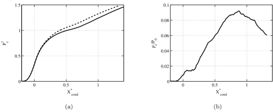
0 0.5 1 0 0.5 1 1.5 Pc * X* cond (a) 0 0.5 1 0 0.02 0.04 0.06 0.08 0.1 p ,/Pc 0 X* cond (b)

FIG. 10. (a) Conditional pressure distributions for small (dashed line) and large (solid line) inter-actions. (b) Difference between the conditional pressures of small and large separations.

for small and large bubbles are reported in figure 10(a), alongside the difference between them in figure 10(b). The dimensionless longitudinal coordinate is defined by X_cond∗ = (x − X0,cond/L), where X0,cond is the mean position of the separation-shock foot related to the classes. The mean values P_C∗ = (PC− P0)/P0, where PC is the average value for the conditional pressures, are denoted on figure 10(a) by the dashed line for the smallest interaction, and full line for the largest interaction. In the frame of the separation shock, the pressure variation p0_C = ∆PC is free from the effects of the translating pressure jump and of the incoherent turbulent fluctuations. It is consequently the pressure variation inherent to the dynamics of the bubble, i.e. the coherent fluctuations whose main features can be summarized as follows:

• within the upstream part of the bubble (0 < X∗

cond < 0.2, lying in region A defined in the wind-tunnel frame of reference), the mean pressure distributions of each case are similar. This means that the pressure jump across the separation shock remains nearly constant, being unaffected by the low-frequency breathing of the bubble. This is consistent with previous observations at low frequencies presented in section III and figure 4(a), where low RMS pressure levels were observed downstream from the separation shock just above the edge of the boundary layer.

• Downstream from the separation point (0.2 < X∗

cond< 0.6), matching region B in the wind-tunnel frame of reference, the difference between mean pressure profiles increases continuously with higher pressure values for the small bubble.

• For 0.6 < X∗ _{< 1.2 (associated with region C), fluctuations somehow level with a} plateau value of p0_C/P0' 0.09.

• Further downstream, the difference between both classes decreases.

Focusing on the upstream part of the bubble, as the separation-shock intensity remains nearly constant regardless of bubble size, the initial part of the interaction can be approxi-mated as a simple translation of the separation point with a nearly constant flow deviation, resulting in the separation shock following the same displacement. Note that this proposal differs from that proposed by Touber and Sandham18_{where the shock motions are directly} related to shock angle variations. Beyond that region, there is no clear pressure plateau but the streamwise evolution for the large bubble more likely tends towards an isobaric behavior, thus making p0_C increases continuously. Then, in the region 0.6 < X∗< 1.2, the maximum value of p0_C/P0≈ 0.09 is reached. This corresponds to p0C/P0≈ 4 × p∗LF, as deduced from the corresponding region in figure 6. Such a value is close to that obtained by assuming

P 0 3 P 1 L P 1 S 0 0,7 0,9 1,0 0 2 4 5 1 X* cond P_c

FIG. 11. Descriptive model of the conditional wall-pressure for small (dashed line) and large bubbles (solid line) in the separation–shock frame. Arrows denote the pressure variations when moving from the large to the small bubble, as plotted in figure 10(b).

a Gaussian distribution for the low-pass filtered pressure fluctuation which yields typical extremal values of ±3 × p0_LF. This acceptable agreement demonstrates that the present conditional analysis is consistent. Finally note that strong pressure fluctuations found in the near–wall region close to the separation point are transmitted to the supersonic region of the interaction following characteristic lines. They are then able to affect the upper part of the separation shock32. This point will be addressed in section V.

C. Global descriptive model for the wall-pressure fluctuations

Taking into account the results described in the previous section, a quasi-static scenario for the evolution of the wall pressure from small to large bubbles is derived from the results detailed in the previous section. It is described in the separation-shock frame in figure 11 with the interaction being split in six regions:

• the upstream region is denoted 0.

• the pressure jump across the separation shock corresponds to region 1.

• region 2 corresponds to the region where the pressure evolution is isobaric for both small and large bubble. Note that even though no clear isobaric region is found from the present data, it could be observed in cases of more intense separations.

• region 3 corresponds to the downstream part of the isobaric region for the large bubble and to the beginning of the pressure gradient found in the interaction for the small bubble.

• region 4 corresponds to the region where a nearly constant adverse pressure gradient is found for both small and large bubbles.

• finally, region 5 corresponds to the downstream region with vanishing adverse pressure gradients.

The same descriptive model is sketched in the wind-tunnel frame in figure 12 and induced phase relationships between the separation–shock location and wall-pressure variations are reported, when defined, in the grey regions. This simple sketch makes it possible to describe the main features of wall-pressure fluctuations identified in previous sections, namely:

• the anti–phase relationship in region A, with large intermittent pressure fluctuations relating to the pressure step across the separation shock.

Lex =0

Φ

Φ

FIG. 12. Descriptive model of the conditional wall–pressure for small (dashed line) and large bubbles (solid line) in the wind-tunnel frame. Grey zones denote the regions in which a constant phase Φ between the shock location and the pressure can be derived from the model. Arrows denote the pressure variations when moving from the large to the small bubble.

• the in–phase relationship in region C and downstream, as long as the adverse gradi-ent pressure does not vanish, with a maximum of the cohergradi-ent pressure fluctuations centered in region C.

• a buffer zone, corresponding to region B where in-phase, anti-phase or null coherent pressure fluctuations can be obtained. As already mentioned, in our case, the isobaric region for small bubbles is vanishing and the extent of the region bounded by black vertical lines in figure 12 is nearly reduced to a point. Therefore, in region B, we observe mainly equiprobable switches from in-phase to anti–phase, and vice versa. This is the reason why no correlation between the wall pressure and the shock motions is obtained in this region. Moreover, in the downstream part of this region, coherent pressure fluctuations should increase from nearly null fluctuations to values of the same order as those in region C, as observed in figure 10.

The scheme of figure 12 makes it possible to describe various levels of pressure fluctua-tions, phase relationships and levels of coherence at the wall along the interaction. These properties are maintained in large regions of the interaction, in particular in the supersonic regions (see figures 4(a) and 5). The next section will verify the ability of this scheme, derived from wall data, to be extended to the supersonic part of the interaction.

V. PRESSURE UNSTEADINESS IN THE SUPERSONIC REGION DOWNSTREAM OF THE SEPARATION SHOCK.

The conditional streamwise pressure profiles can be analyzed in the supersonic region of the interaction by using the same approach as that described in section IV B for wall pressure. The region under consideration is located above y = HI , i.e. above the crossing point for the incident and the separation shocks, in order to focus on the outer, supersonic part of the flow. The same two conditioning classes as for wall pressure are used and correspond respectively to small and large bubbles. The conditionally–averaged pressure at the same dimensionless altitude Y /HI = 1.3 is reported in figure 13. The solid and dashed lines correspond to large and small bubbles, respectively. The origin for the longitudinal coordinate is set at the mean location for the incident shock at the same altitude, denoted X1.

The pressure immediately downstream from the incident shock is nearly constant for both cases, demonstrating that separation-shock intensity can also be considered as nearly constant in this region. A second pressure bump is found just upstream from the expansion

0.02 0.03 0.04 0.05 0.06 0.07 0.08 0.5 1 1.5 2 2.5 P C * X−X l [m]

FIG. 13. Conditional mean pressure profiles obtained at Y /HI = 1.3 for small (dashed line) and

large (solid line) bubbles.

wave, regardless of the interaction size, and its intensity increases for small bubbles. The pressure difference upstream from the expansion wave between the small and large bubbles is about 6.9×10−2P0and it is maintained beyond the expansion fan. Therefore the intensity of the expansion wave can be considered as independent of the state of separation.

The second pressure bump must be associated with the crossing of compression waves developing between the separation shock and the expansion wave, see figures 1(a) and 4(a). As previously mentioned, they emanate from the reflection of the incident shock on the sonic line36_{, as shown by a dashed line in figure 4(a).}

At this point in the analysis, it seems that pressure fluctuations in the external flow follow the dynamics in the separated region. As the external flow is supersonic relative to the separated region, pressure perturbations will spread out along the directions defined by the characteristics32_{. This implies that low-frequency pressure fluctuations emanating} from region B can influence the separation–shock region up to its intersection with the compression waves, denoted Hwin figure 1(b), while the fluctuations emanating from region C will influence the shock above Hw.

In previous sections, it has been seen that low levels of coherent pressure fluctuations are encountered in region A and at the beginning of region B. Consequently, when consider-ing the separation–shock frame, the shock system remains nearly constant below HI since ascending–characteristic lines, whose feet are located in those regions, cross the separation shock below that point. On the other hand, coherent pressure fluctuations of higher ampli-tude developing in the downstream part of region B and in region C lead to an increase in pressure for small bubbles. The beginning of region C corresponds to the reflection of the incident shock on the shear layer. As the shear layer is subject to the low–frequency fluctu-ations of its upstream condition, the intensity of the reflected compression waves, created just upstream of the expansion wave, is also modulated at low-frequency.

As shown in figure 13, the pressure difference between the two conditional means remains constant throughout the expansion fan, this implies that low-frequency pressure fluctua-tions in the supersonic region are in phase with their subsonic counterparts in region C. Eventually, compression waves merge with the separation shock for Y > Hw. This suggests that, in region C, the intensity of the shock system varies according to the size of the in-teraction: separation-shock intensity remains nearly constant, but is strengthened by the compression waves. As the compression-wave magnitude depends on the bubble-size state, pressure increases across the equivalent shock and is regulated by the bubble breathing.

00000000000000000000000000000000000000000000 11111111111111111111111111111111111111111111 C 3 C 4 C 1 ϕ 1 ϕ 3 ϕ ϕ A B C C 2 1 2 3 4 I H ϕ₂ χ D D 0 Expansion fan

Isobaric region"Dead air"

FIG. 14. Inviscid equivalent scenario for shock-wave boundary layer interaction with separation25.

In the next section, a conceptual inviscid view of low-frequency unsteadiness developing the interaction is proposed. It is built in order to take into account all the features described thus far.

VI. CONCEPTUAL MODEL OF EQUIVALENT INVISCID INTERACTION A. Reminder: free interaction theory

An inviscid equivalent scheme of the shock-wave/boundary-layer interaction has already been proposed by Delery and Marvin25_{and is sketched in figure 14. The separation region} is assimilated with an isobaric region divided in two parts:

• the upstream region extends from the separation point to the reflection of the incident shock on the separated region. This region corresponds to a constant positive deviation angle.

• The downstream region is associated with a constant negative angle in order to en-sure the flow reattachment. It yields the creation of an expansion wave. Presen-sure equilibrium between the isobaric separation and the supersonic regions is obtained by ensuring that the pressure decrease across the expansion wave is equal to its increase across the incident shock. Thus, expansion deviates the flow down to the wall at an angle approximatively equal to the incident shock and P2' P4.

Downstream from the reattachment, an equivalent reattachment shock is required to model the flow deviation necessary for achieving a wall–parallel streamline. It results in the in-crease in pressure found downstream from the interaction. When the interaction is fully sep-arated, the deflection angle imposed by the first ramp becomes independent of the incident– shock intensity and consequently the pressure ratio at the separation point also becomes independent. Similar features were found for compression ramps41_{, in accordance with the} so–called free interaction theory42_.

As shown in section IV A, the whole separated region cannot be associated with an isobaric region since only region B exhibits a pressure gradient close to zero. In the second part of the separated region (subregion C), a significant adverse pressure gradient develops and is associated with large unsteady pressures (see figure 10(b)). Moreover, it has been shown, in section V, that the shock system balances the pressure between the subsonic and supersonic regions by means of reflected compression waves produced by reflection of the incident shock through the boundary layer36_{. Such compression waves, seen in figure 1(a)}

00000000000000000000000000000000000000000000 11111111111111111111111111111111111111111111 C 2 C 1 ϕ 1 ϕ₂ 0 1 C 3 C 3’ 2 3 3’ ϕD ϕ D 4’ C 4’ C 4 H w χ Expansion fan

(a)Large separated region

00000000000000000000000000000000000000000000 11111111111111111111111111111111111111111111 C 1 ϕ 1 0 4’’ 1 C 2 ϕ 2 2 C 3 ϕ D ϕ D C 4’’ 3’’ C 4 H w χ Expansion fan

(b)Small separated region

FIG. 15. Possible inviscid equivalent scenario of the shock wave boundary layer interaction de-pending on the interaction length.

as dark lines located upstream from the expansion fan, are inconsistent with the single ramp scenario described in figure 14.

A new conceptual model, sketched in figure 15(a), is introduced to alleviate these short-comings. A new second ramp is added just upstream from the impingement point of the incident-shock. It splits the equivalent subsonic region into two parts which can be asso-ciated respectively with regions B and C of the scheme introduced in figure 12. The first ramp results in a flow deflection compatible with the free interaction theory, i.e. indepen-dent of the size of the separation. The flow then undergoes a second deviation, due to the second ramp, and imposes an increase in pressure. In the inviscid supersonic region, this leads to the creation of the shock C₃0 which intersects the separation shock C4near Hw, thus strengthening the separation shock up to the value C₄0. In the next section, this conceptual model is extended to include the different states of the subsonic separated bubble.

B. Description of the quasi-static scenario

Results described in section V when analyzing figure 13 indicate that the intensity of the equivalent shock C₃0 depends on the bubble size: its intensity, or its equivalent the flow deviation of the second ramp in the model, is lower for large bubbles than for small bubbles. Figure 15(a), being from now on associated with large bubbles, is consequently complemented by figure 15(b), which corresponds to small bubbles with a second ramp steeper than for large bubbles. Note that this conceptual model is built from observed results but that the physical cause of such a pressure increase for small bubbles remains unclear.

The modeling may be further refined by noting that the frequencies associated with the breathing of the separated region are at least one order of magnitude lower than the frequencies related to both the mixing layer and the incoming turbulence. It is therefore proposed to model the low-frequency kinematics of the interaction in a quasi-static way by moving from large to small bubbles and vice-versa. For a growing bubble, the dynamics of the interaction can be modeled in the following quasi–static way:

• the separation point is translated in the upstream direction, with a constant flow– deviation angle and a translation velocity negligible with respect to the upstream velocity.

• As the deviation angle does not change and as the translation velocity is low, the separation-shock intensity remains constant. The shock is therefore simply translated

• Within the second part of the bubble, the pressure gradient weakens, as seen in figure 10(b).

• As the pressure decreases, the compression–wave arising from the refraction of the incident shock through the mixing layer weakens.

• As the expansion wave does not change, the pressure behind the shock system is also reduced.

• Finally, the reattachment shock ensures that the flow turns parallel to the wall and balances the downstream pressure

The inverse procedure develops when the bubble contracts.

Such a scenario extends the scheme built from the wall pressure in figure 12 to the super-sonic regions. It also describes the unsteadiness features of the interaction and explains how the shock system depends on the separated zone. It is also consistent with the coherence map in figure 5: large coherence is observed between the low-frequency shock displacements (or bubble breathing) and the expansion, compression waves, and the downstream supersonic regions. On the other hand, in the intermediate region, upstream from the compression waves, no correlation is observed and there are only limited fluctuations in pressure.

The low-frequency unsteadiness of the first ramp can be associated with the bubble breathing, which is linked to the extent of region B with a small or null pressure gradient (isobaric region in cases of large separated bubbles). This is the origin of the longitudinal displacements of the separation shock, and could be explained by an imbalanced mass flux across the initial part of the mixing layer21_{. On the other hand, the second ramp} unsteadi-ness involves a specific region of the interaction, typically 0.6 < X∗ _{< 0.8, see figure 10.} This corresponds to region C, where large pressure gradients are observed, downstream from the nearly isobaric region, as in subsonic separated cases. This pressure gradient en-sures the connection with downstream pressure in the separated region and generates weak pressure fluctuations at low frequency, as proposed by the schemes in figure 15.

VII. DISCUSSION

This conceptual model makes it possible to describe the streamwise evolution of pressure as a function of the interaction length, but is restricted to low-passed-filtered data. However several authors have pointed out the importance of convective structures produced by the shear layer and induced by the decelerated region in the mechanism that generates the low–frequency unsteadiness for incompressible flows43–45 _{and for compressible flows}21_{. As} a consequence, the model’s compatibility with medium-frequency unsteadiness (Strouhal number ranging from 0.5 to 1.0) will be considered in this section. It is shown that the model introduced above can describe the different pressure variation features found in compressible flows and can be extended to incompressible flows.

A. Attempt to establish similarity between incompressible and compressible separation bubbles Several experiments and numerical simulations have shown that large structures are de-veloping in the shear layer downstream from the separation point. Spatial development of these structures has been compared with incompressible separated flows and large sim-ilarities were highlighted5_{, with two distinct frequency ranges in the upstream part of the} separated region (region B introduced in this paper) and the downstream part (region C). Region C was associated with the development of large structures that were shed down-stream, as in subsonic cases. A typical Strouhal number SL' 0.5 was associated with the

−0.50 0 0.5 1 1.5 2 0.005 0.01 0.015 0.02 0.025 0.03 0.035 0.04 x* p’ / .5 ρ0 U 0 2 Present Lee&Sung (2001) Le and Moin (1994)

FIG. 16. Streamwise evolution of the RMS pressure in separated flows. Solid line: present work; dashed-dotted lines: subsonic backward facing steps from experiments49 _{(•) and DNS}50

(N).

frequencies of the shedding, typically one order of magnitude higher than the low frequen-cies of the shock motions (SL ' 0.03). Evidence of low-frequency variations of the typical velocity profiles and wall shear stress related to some large coherent scales were also found in the case of a Mach 2.9 compression corner with separation17_{. Piponniau et al.}21_developed a model which links mass entrainment associated with the development of these structures to low-frequency breathing of the separated region, an idea already suggested in several subsonic works46–48. This model is suitable for incompressible and compressible separated flows, even though it underlines the major effects of compressibility on low-frequency un-steadiness. These results suggest that there are large similarities between incompressible and compressible separated flows. In the present work, pressure–field analysis makes it possible to take an additional view of these similarities.

Lee and Sung49 have compiled several results obtained from separated subsonic flows for backward step flows. The corresponding streamwise RMS are reported in figure 16. Pressure fluctuations have been normalized by upstream dynamic pressure q0. For comparisons with the present results, figure 16 is zoomed and centered on the separated region displayed in figure 10(b) and corresponding to regions B and C. Coherent pressure fluctuations are normalized with the dynamic pressure obtained downstream from the incident shock C1. The dimensionless longitudinal coordinate Xsep is defined by (x − X0)/Lsep, where Lsep is the length of separation and X0the separation point, associated with the mean position of the separation shock in the compressible case.

The different subsonic cases reported in figure 16 correspond to various backward-facing steps. Two important points should be emphasized. First, subsonic measurements are given in the wind-tunnel frame. Nevertheless, in cases of backward-facing steps, the separation point is fixed at the corner of the step. Therefore, the conditional analysis developed in the previous section, which tries to remove the influence of moving the separation point linked to separation-shock displacements, makes it possible to compare the present compressible conditional analysis with an incompressible compilation49. The second important point is that only the coherent part of the pressure fluctuations has been evaluated, while subsonic results correspond to broadband measurements: therefore, the level of fluctuations cannot be directly compared on an absolute basis.

Nevertheless, it is clear that large similarities can be observed between compressible and incompressible situations. In both cases, the separated region is split in two parts, as suggested in figure 11, with:

0.15 0.15 0.15 0.15 0.15 0.15 0.15 0.2 0.2 0.2 0.2 0.2 0.2 0.25 0.25 0.25 0.25 _0.3 0.3 0.3 0.35 0.35 0.4 0.4 Y/H I X* 0 0.5 1 1.5 0.5 1 1.5 2 0 0.2 0.4 0.6 0.8 1

C

B

A

FIG. 17. Coherence for SL= 0.5 between the wall-pressure fluctuations at the normalized

stream-wise location X∗and the separation-shock displacement at the normalized altitude Y /HI.

• the upstream part with limited pressure gradient, associated with the inflection point in the pressure distribution and average, increasing, pressure fluctuations (in region B),

• the downstream part, characterized by a stronger adverse pressure gradient related to stronger, leveling, pressure fluctuations (in region C).

Region C seems to be related to the development of large coherent scales, shed down-stream from the interaction, and associated with large turbulent pressure fluctuations oc-curring in that region. It can therefore be reasonably assumed that the dynamics of large coherent scales along the shear layer is associated with coherent pressure fields shown in figure 16. Consequently a reasoning analogous to those relating to the low-frequency bub-ble breathing could describe the influence of pressure fluctuations associated with coherent scales (SL' 0.5) on shock displacement at medium frequencies. This point is addressed in the following section.

B. Generalisation of the inviscid model to medium frequencies

Previous works32,51, show that organized convective structures are produced within the shear layer,and are associated with Strouhal numbers ranging from 0.5 to 1.0. These struc-tures convect with a relative supersonic velocity with respect to the supersonic side of the interaction and the pressure disturbances generated by convective structures and propa-gation paths have been clearly defined. These results are summarized in figure 17 by the map of the coherence at SL= 0.5 between the longitudinal shock motion at given altitudes and the wall pressure at given streamwise locations. This map sheds light on the links be-tween the separation-shock displacement and the medium-frequency pressure fluctuations induced by the convective structures, as seen in figure 7 for the link between shock motion and low-frequency unsteadiness.

• In the first part of the interaction, the structures produced by the shear layer are con-vected, and the pressure disturbances affect the separation-shock dynamics. Through-out their displacements in the region X∗ < 0.5, the pressure fluctuations produced by the convective structures propagate along Mach waves and influence the region

X* Y/H I 0 0.5 1 0 0.5 1 1.5 2 0.025 0.0375 0.050 0.0625

FIG. 18. RMS range-filtered pressure fluctuations corresponding to medium frequency with Strouhal numbers ranging from 0.3 and 0.8. The sonic line is denoted by a dashed line. The dotted line corresponds to the incident and separation shocks and the dashed-dotted lines mark the boundaries of the expansion fan.

below the crossing point between the separation shock and the expansion waves. It is consistent with the fact that the coherence coefficient increases with the altitude in region B, as seen in figure 17.

• In region C, wall-pressure variations and separation-shock dynamics have the strongest coherent-coefficient level at high altitude. It has to be noted that any modulation of upstream conditions in the lower part of the incident shock will affect its reflection in compression waves in such a way as to balance the pressure fields imposed by the sub-sonic region32,36_{. Consequently, the large coherent scales developing in region B and} then crossing the adverse pressure gradient found at the beginning of region C mod-ulate the separation-shock intensity through the compression waves propagating just upstream from the expansion fan. It results in the high level of coherence mentioned earlier, see figure 17.

The influence of medium-frequency coherent structures on the reflection of incident shock can be verified by examining figure 18. This shows RMS pressure values for the medium frequency range 0.3 < SL < 0.8. Average values induced by the convection of coherent structures along the mixing layer are found in region B while the foot of the incident shock/reflected compression waves experiences much higher values. Large values are also recovered along the path of compression waves up to the location Hwat which they intercept the separation shock, in agreement with the characteristics–based analysis of the propaga-tion of pressure disturbances coming from the foot of the incident shock, as developed in Agostini et al.32.

Based on these findings regarding the strong values of pressure fluctuation at medium frequencies over the whole region of the compression waves, the inviscid equivalent model sketched in figure 15 can be extended to the medium-frequency unsteadiness. It is achieved by linking the medium-frequency unsteadiness to the second ramp in order to include the pressure variations due to the interaction of the convective structures with the adverse pressure gradient of region C.

The newly–defined model encompassing both the low– and medium–frequency phenomena is illustrated in figure 19. The first ramp (region B) follows the low–frequency unsteadiness of the separation point (region A), and convective structures develop in this region, thus influencing the separation shock through the Mach lines32_{. When these structures enter the} vicinity of the second ramp (region C), their dynamics change abruptly5. These variations could be linked to the pressure gradient represented by the second ramp, while the intensity of the second ramp could be affected by the new convective-structure dynamics. Therefore,

00000000000000000000000000000000000000000000 11111111111111111111111111111111111111111111 H w LF and MF ZONE OF

FIG. 19. Conceptual inviscid model of sources for the low and medium frequency unsteadiness in the interaction

the second ramp, associated with region C in the scheme of figure 19, displays oscillations at two different characteristic frequencies:

• low frequency with SL' 0.03, associated with the bubble breathing,

• a medium frequency with SL' 0.5, associated with the convective structures and the rapid decrease in their time scale in this region.

The resulting unsteady pressure field at low and medium frequencies compares well with LES data taking into account the fact that the outer flow unsteadiness is derived from unsteadiness in the subsonic region through the theory of characteristics32_{. In particular,} the phase relationships, the coherence maps and the evolution of the pressure standard deviation are qualitatively reproduced.

It should be stressed that the scheme presented does not explain the origin of low-frequency unsteadiness, which could be induced by medium low-frequency unsteadiness, as suggested by several authors, both for subsonic45,47,52 _{and supersonic flows}17,21_{. However} no direct link between low-frequency unsteadiness in the interaction and convective struc-tures in the mixing layer at medium frequencies has been established for the present flow so far. Nonetheless, whatever the precise mechanism linking the two frequency ranges, the proposed simple inviscid scheme will describe accurately the whole field of unsteady pressure within and downstream from the interaction.

VIII. CONCLUSION

Large Eddy Simulations of a Mach 2.3 shock reflection on a turbulent boundary layer with shocks strong enough to induce separated interactions have been used in order to gain insight into the kinematics of both separated and potential regions of the flow. Statistically reliable analyses are made possible by long-time computations which can describe more than 150 cycles of low–frequency unsteadiness in the interaction, characterized by a Strouhal number roughly equal to 0.03. Moreover this numerical database has already accurately described low– and medium–frequency unsteadiness of the flow when compared with experimental data obtained in the same aerodynamic conditions.

Spectral and conditional analyses of the pressure fields have given a global overview of the flow’s space–time organization. Based on these data, an equivalent inviscid scheme is introduced and summarized in figure 19. It allows the reproduction of essential properties for pressure variations within and downstream from the interaction.

This conceptual model is able to mimic the shock–system unsteadiness at low frequencies (SL= 0.03) and medium frequencies (SL= 0.5). Displacement of the upstream part of the

separated region is described as a simple corner translation. Therefore, the separation shock induced by this flow deviation moves with a nearly constant intensity. The second part of the separated zone is the source of pressure fluctuations which influence the supersonic region of the interaction. This is described as a second unsteady flow deviation depending on the bubble size, although the physical nature of the mechanism inducing these fluctuations remains an open question. It is important to stress that this second ramp is a conceptual inviscid view of the phenomena occurring in the real flow. One possible explanation for these phenomena could be the viscous refraction process described by Henderson36 but further investigation would be required to confirm that point. This scheme is nonetheless able to give justification for the regions identified from RMS pressure fields and from coherence function with the shock motion even though it does not provide a prediction of the actual low– and medium–frequency ranges at which the aforementioned phenomena occur.

Moreover, it is shown that the separation-shock undergoes only a translation motion with negligible variation of its intensity. Nevertheless, in the region located above the intersection with the incident shock, the separation-shock intensity is strengthened by the merging of unsteady pressure waves which are emitted from the shedding region at low and medium frequencies. It generates unsteady pressure fluctuations downstream from the expansion wave and these are in phase with the displacement of the separation shock.

Previous works17,21_{have suggested possible interactions between bubble breathing at low} frequency and convective structures associated with medium frequencies, without clearly establishing a link between these two frequency ranges. If such interactions indeed exist, the fact that strong flow modulations are found in region C for both frequency ranges could be an indication that these interaction occur in that region. It seems therefore that a detailed statistical space-time description of these convective structures could be a key point for understanding low-frequency unsteadiness in separated flows. This remark holds for both incompressible and compressible flows since it appears from the present research that shock-system unsteadiness is merely a passive “slave” of dynamics developed in the separated region.

IX. ACKNOWLEDGMENTS

This work was partly supported by the Agence National de la Recherche (ANR) through the DECOMOS project from the Blanc program. The research team was granted access to high–performance computing resources of Institut du D´eveloppement et des Ressources en Informatique Scientifique (IDRIS) under allocations 2009-021877 and 2010-021877 made by Grand Equipement National de Calcul Intensif (GENCI).

1_{M. E. Erengil and D. S. Dolling, “Unsteady wave structure near separation in a Mach 5 compression ramp} interaction,” AIAA Journal 29, 728–735 (1991).

2_{F. O. Thomas, C. M. Putman, and H. C. Chu, “On the mechanism of unsteady shock oscillation in shock} wave/turbulent boundary layer interaction,” Experiments in Fluids 18, 69–81 (1994).

3_{D. S. Dolling, “Fifty years of shock-wave/boundary-layer interaction research: what next,” AIAA Journal} 39, 1517–1531 (2001).

4_{S. J. Beresh, N. T. Clemens, and D. S.Dolling, “Relationship between upstream turbulent boundary layer} velocity fluctuations and separation shock unsteadiness,” AIAA Journal 40, 2412–2422 (2002).

5_{P. Dupont, C. Haddad, and J. F. Debi`eve, “Space and time organization in a shock induced boundary} layer,” Journal of Fluid Mechanics 559, 255–277 (2006).

6_{B. Ganapathisubramani, N. Clemens, and D. Dolling, “Effects of upstream boundary layer on the} un-steadiness of shock-induced separation,” Journal of Fluid Mechanics 585, 369–394 (2007).

7_{N. T. Clemens and V. Narayanaswamy, “Low-Frequency Unsteadiness of Shock Wave/Turbulent} Bound-ary Layer Interactions,” Annual Review of Fluid Mechanics 46, 469–492 (2014).

8_{M. Wu and M. P. Martin, “Analysis of shock motion in shockwave and turbulent boundary layer} interac-tion using direct numerical simulainterac-tion data,” Journal of Fluid Mechanics 594, 71–83 (2008).

9_{E. Touber and N. D. Sandham, “Large–eddy simulation of low–frequency unsteadiness in a turbulent} shock–induced separation bubble,” Theoretical and Computational Fluid Dynamics 23, 79–107 (2009). 10_{B. Morgan, K. Duraisamy, N. Nguyen, S. Kawai, and S. K. Lele, “Flow physics and RANS modelling of}