A Constraint Solver for Software Engineering:
Finding Models and Cores of Large Relational
Specifications
by
Emina Torlak
M.Eng., Massachusetts Institute of Technology (2004) B.Sc., Massachusetts Institute of Technology (2003)
Submitted to the Department of Electrical Engineering and Computer
Science
in partial fulfillment of the requirements for the degree of
Doctor of Philosophy
at the
MASSACHUSETTS INSTITUTE OF TECHNOLOGY
February 2009
c
Massachusetts Institute of Technology 2009. All rights reserved.
Author . . . .
Department of Electrical Engineering and Computer Science
December 16, 2008
Certified by . . . .
Daniel Jackson
Professor
Thesis Supervisor
Accepted by . . . .
Professor Terry P. Orlando
Chairman, Department Committee on Graduate Students
A Constraint Solver for Software Engineering: Finding
Models and Cores of Large Relational Specifications
by
Emina Torlak
Submitted to the Department of Electrical Engineering and Computer Science on December 16, 2008, in partial fulfillment of the
requirements for the degree of Doctor of Philosophy
Abstract
Relational logic is an attractive candidate for a software description language, be-cause both the design and implementation of software often involve reasoning about relational structures: organizational hierarchies in the problem domain, architectural configurations in the high level design, or graphs and linked lists in low level code. Un-til recently, however, frameworks for solving relational constraints have had limited applicability. Designed to analyze small, hand-crafted models of software systems, current frameworks perform poorly on specifications that are large or that have par-tially known solutions.
This thesis presents an efficient constraint solver for relational logic, with recent applications to design analysis, code checking, test-case generation, and declarative configuration. The solver provides analyses for both satisfiable and unsatisfiable specifications—a finite model finder for the former and a minimal unsatisfiable core extractor for the latter. It works by translating a relational problem to a boolean satisfiability problem; applying an off-the-shelf SAT solver to the resulting formula; and converting the SAT solver’s output back to the relational domain.
The idea of solving relational problems by reduction to SAT is not new. The core contributions of this work, instead, are new techniques for expanding the capacity and applicability of SAT-based engines. They include: a new interface to SAT that extends relational logic with a mechanism for specifying partial solutions; a new translation algorithm based on sparse matrices and auto-compacting circuits; a new symmetry detection technique that works in the presence of partial solutions; and a new core extraction algorithm that recycles inferences made at the boolean level to speed up core minimization at the specification level.
Thesis Supervisor: Daniel Jackson Title: Professor
Acknowledgments
Working on this thesis has been a challenging, rewarding and, above all, wonderful experience. I am deeply grateful to the people who have shared it with me:
To my advisor, Daniel Jackson, for his guidance, support, enthusiasm, and a great sense of humor. He has helped me become not only a better researcher, but a better writer and a better advocate for my ideas.
To my thesis readers, David Karger and Sharad Malik, for their insights and excellent comments.
To my friends and colleagues in the Software Design Group—Felix Chang, Greg Dennis, Jonathan Edwards, Eunsuk Kang, Sarfraz Khurshid, Carlos Pacheco, Derek Rayside, Robert Seater, Ilya Shlyakhter, Mana Taghdiri and Mandana Vaziri—for their companionship and for many lively discussions of research ideas, big and small. Ilya’s work on Alloy3 paved the way for this disserta-tion; Greg, Mana and Felix’s early adoption of the solver described here was instrumental to its design and development.
To my husband Aled for his love, patience and encouragement; to my sister Alma for her boundless warmth and kindness; and to my mother Edina for her unrelenting support and for giving me life more than once.
The first challenge for computing science is to discover how to maintain order in a finite, but very large, discrete universe that is intricately intertwined. E. W. Dijkstra, 1979
Contents
1 Introduction 13
1.1 Bounded relational logic . . . 15
1.2 Finite model finding . . . 17
1.3 Minimal unsatisfiable core extraction . . . 23
1.4 Summary of contributions . . . 27
2 From Relational to Boolean Logic 31 2.1 Bounded relational logic . . . 32
2.2 Translating bounded relational logic to SAT . . . 35
2.2.1 Translation algorithm . . . 35
2.2.2 Sparse-matrix representation of relations . . . 37
2.2.3 Sharing detection at the boolean level . . . 40
2.3 Related work . . . 44
2.3.1 Type-based representation of relations . . . 44
2.3.2 Sharing detection at the problem level . . . 46
2.3.3 Multidimensional sparse matrices . . . 47
2.3.4 Auto-compacting circuits . . . 50
2.4 Experimental results . . . 51
3 Detecting Symmetries 55 3.1 Symmetries in model extension . . . 56
3.2 Complete and greedy symmetry detection . . . 60
3.2.2 Symmetries via greedy base partitioning . . . 63
3.3 Experimental results . . . 68
3.4 Related work . . . 70
3.4.1 Symmetries in traditional model finding . . . 71
3.4.2 Symmetries in constraint programming . . . 72
4 Finding Minimal Cores 75 4.1 A small example . . . 76
4.1.1 A toy list specification . . . 76
4.1.2 Sample analyses . . . 77
4.2 Core extraction with a resolution engine . . . 81
4.2.1 Resolution-based analysis . . . 82
4.2.2 Recycling core extraction . . . 86
4.2.3 Correctness and minimality of RCE . . . 88
4.3 Experimental results . . . 89
4.4 Related work . . . 93
4.4.1 Minimal core extraction . . . 93
4.4.2 Clause recycling . . . 94
5 Conclusion 97 5.1 Discussion . . . 98
5.2 Future work . . . 101
5.2.1 Bitvector arithmetic and inductive definitions . . . 101
5.2.2 Special-purpose translation for logic fragments . . . 102
List of Figures
1-1 A hard Sudoku puzzle . . . 13
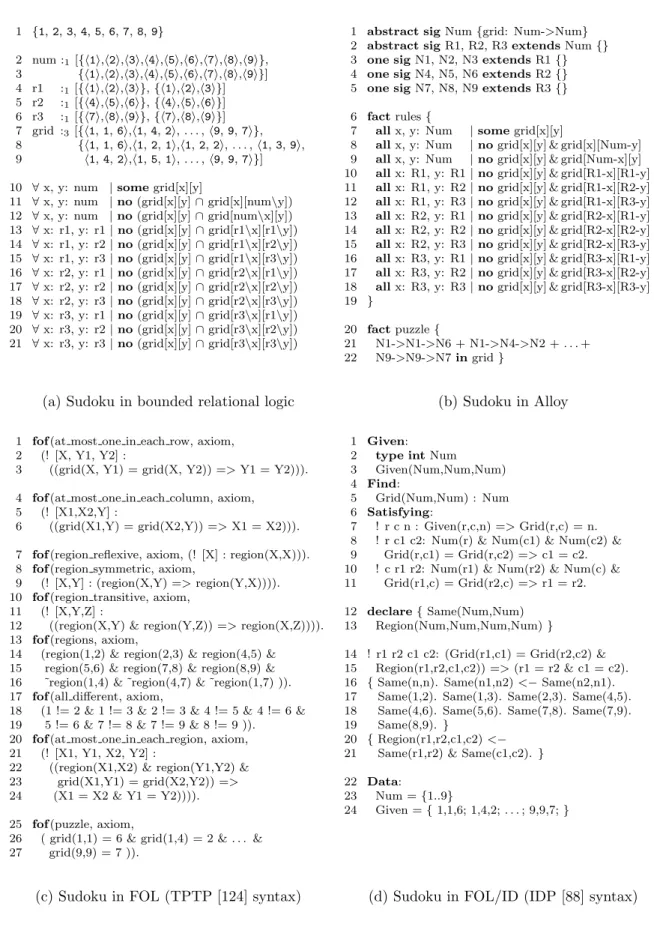
1-2 Sudoku in bounded relational logic, Alloy, FOL, and FOL/ID . . . 18
1-3 Solution for the sample Sudoku puzzle . . . 19
1-4 Effect of partial models on the performance of SAT-based model finders . 21 1-5 Effect of partial models on the performance of a dedicated Sudoku solver . 22 1-6 An unsatisfiable Sudoku puzzle and its core . . . 24
1-7 Comparison of SAT-based core extractors on 100 unsatisfiable Sudokus . . 26
1-8 Summary of contributions . . . 28
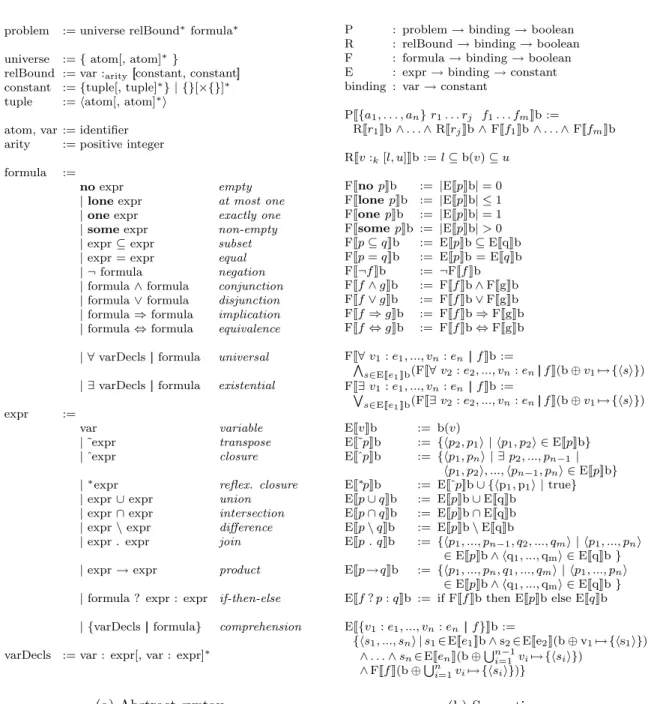
2-1 Syntax and semantics of bounded relational logic . . . 33
2-2 A toy filesystem . . . 34
2-3 Translation rules for bounded relational logic . . . 36
2-4 A sample translation . . . 38
2-5 Sparse representation of translation matrices. . . 39
2-6 Computing the d-reachable descendants of a CBC node . . . 41
2-7 A non-compact boolean circuit and its compact equivalents . . . 43
2-8 GCRS and ECRS representations for multidimensional sparse matrices . . 48
2-9 An example of a non-optimal two-level rewrite rule . . . 52
3-1 Isomorphisms of the filesystem model . . . 57
3-2 Isomorphisms of an invalid binding for the toy filesystem . . . 57
3-3 Complete symmetry detection via graph automorphism . . . 62
3-4 A toy filesystem with no partial model . . . 64
3-6 Microstructure of a CSP . . . 74
4-1 A toy list specification . . . 78
4-2 The resolution rule for propositional logic . . . 84
4-3 Resolution-based analysis of (a = b) ∧ (b = c) ∧ ¬(a ⇒ c) . . . 84
List of Tables
1.1 Recent applications of Kodkod . . . 29
2.1 Simplification rules for CBCs. . . 42
2.2 Evaluation of Kodkod’s translation optimizations . . . 53
3.1 Evaluation of symmetry detection algorithms . . . 69
4.1 Evaluation of minimal core extractors . . . 90
4.2 Evaluation of minimal core extractors based on problem difficulty . . . 91
Chapter 1
Introduction
Puzzles with simple rules can be surprisingly hard to solve, even when a part of the solution is already known. Take Sudoku, for example. It is a logic game played on a partially completed 9 × 9 grid, like the one in Fig. 1-1. The goal is simply to fill in the blanks so that the numbers 1 through 9 appear exactly once in every row, column, and heavily boxed region of the grid. Each puzzle has a unique solution, and many are easily solved. Yet some are ‘very hard.’ Target completion time for the puzzle in Fig. 1-1, for example, is 30 minutes [58].
6 2 5 1 8 6 2 3 4 6 7 8 4 2 5 9 8 5 4 9 3 2 1 4 3 5 7
Figure 1-1: A hard Sudoku puzzle [58].
Software engineering is full of problems like Sudoku—where the rules are easy to describe, parts of the solution are known, but the task of filling in the blanks is computationally intractable. Examples include, most notably, declarative configura-tion problems such as network configuraconfigura-tion [99], installaconfigura-tion management [133], and
scheduling [149]. The configuration task usually involves extending a valid config-uration with one or more new components so that certain validity constraints are preserved. To install a new package on a Linux machine, for example, an installa-tion manager needs to find a subset of packages in the Linux distribuinstalla-tion, including the desired package, which can be added to the installation so that all package de-pendencies are met. Also related are the problems of declarative analysis: software design analysis [69], bounded code verification against rich structural specifications [31, 34, 126, 138], and declarative test-case generation [77, 114, 134].
Automatic solutions to problems like Sudoku and declarative configuration usually come in two flavors: a special-purpose solver or a special-purpose translator to some logic, used either with an off-the-shelf SAT solver or, since recently, an SMT solver [38, 53, 9, 29] that can also reason about linear integer and bitvector arithmetic. An expertly implemented special-purpose solver is likely to perform better than a translation-based alternative, simply because a custom solver can be guided with domain-specific knowledge that may be hard (or impossible) to use effectively in a translation. But crafting an efficient search algorithm is tricky, and with the advances in SAT solving technology, the performance benefits of implementing a custom solver tend to be negligible [53]. Even for a problem as simple as Sudoku, with many known special-purpose inference rules, SAT-based approaches [86, 144] are competitive with hand-crafted solvers (e.g. [141]).
Reducing a high-level problem description to SAT is not easy, however, since a boolean encoding has to contain just the right amount and kind of information to elicit the best performance from the SAT solver. If the encoding includes too many redundant formulas, the solver will slow down significantly [119, 139, 41]. At the same time, introducing certain kinds of redundancy into the encoding, in the form of symmetry breaking [27, 116] or reconvergence [150] clauses, can yield dramatic improvements in solving times.
The challenges of using SAT for declarative configuration and analysis are not limited to finding the most effective encoding. When a SAT solver fails to find a satisfying assignment for the translation of a problem, many applications need to
know what caused the failure and correct it. For example, if a software package cannot be installed because it conflicts with one or more existing packages, a SAT-based installation manager such as OPIUM [133] needs to identify (and remove) the conflicting packages. It does this by analyzing the proof of unsatisfiability produced by the SAT solver to find an unsatisfiable subset of the translation clauses known as an unsatisfiable core. Once extracted from the proof, the boolean core needs to mapped back to the conflicting constraints in the problem domain. The problem domain core, in turn, has to be minimized before corrective action is taken because it may contain constraints which do not contribute to its unsatisfiability.
This thesis presents a framework that facilitates easy and efficient use of SAT for declarative configuration and analysis. The user of the framework provides just a high-level description of the problem—in a logic that underlies many software design languages [2, 143, 123, 69]—and a partial solution, if one is available. The framework then does the rest: efficient translation to SAT, interpretation of the SAT instance in terms of problem-domain concepts, and, in the case of unsatisfiability, interpretation and minimization of the unsatisfiable core. The key algorithms used for SAT encoding [131] and core minimization [129] are the main technical contributions of this work; the main methodological contribution is the idea of separating the description of the problem from the description of its partial solution [130]. The embodiment of these contributions, called Kodkod, has so far been used in a variety of applications for declarative configuration [100, 149], design analysis [21], bounded code verification [31, 34, 126], and automated test-case generation [114, 134].
1.1
Bounded relational logic
Kodkod is based on the “relational logic” of Alloy [69], consisting essentially of a first-order logic augmented with the operators of the relational calculus [127]. The inclusion of transitive closure extends the expressiveness beyond standard first-order logics, and allows the encoding of common reachability constraints that otherwise could not be expressed. In contrast to specification languages (such as Z [123], B
[2], and OCL [143]) that are based on set-theoretic logics, Alloy’s relational logic was designed to have a stronger connection to data modeling languages (such as ER [22] and SDM [62]), a more uniform syntax, and a simpler semantics. Alloy’s logic treats everything as a relation: sets as relations of arity one and scalars as singleton sets. Function application is modeled as relational join, and an out-of-domain application results in the empty set, dispensing with the need for special notions of undefinedness. The use of multi-arity relations (in contrast to functions over sets) is a critical factor in Alloy being first order and amenable to automatic analysis. The choice of this logic for Kodkod was thus based not only on its simplicity but also on its analyzability.
Kodkod extends the logic of Alloy with the notion of relational bounds. A bounded relational specification is a collection of constraints on relational variables of any arity that are bound above and below by relational constants (i.e. sets of tuples). All bounding constants consist of tuples that are drawn from the same finite universe of uninterpreted elements. The upper bound specifies the tuples that a relation may contain; the lower bound specifies the tuples that it must contain.
Figure 1-2a shows a snippet of bounded relational logic1 that describes the Sudoku
puzzle from Fig. 1-1. It consists of three parts: the universe of discourse (line 1); the bounds on free variables that encode the assertional knowledge about the problem (lines 2-7), such as the initial state of the grid; and the constraints on the bounded variables that encode definitional knowledge about the problem (lines 10-21), i.e. the rules of the game.
The bounds specification is straightforward. The unary relation num (line 2) provides a handle on the set of numbers used in the game. As this set is constant, the relation has the same lower and upper bound. The relations r1, r2 and r3 (lines 4-6) partition the numbers into three consecutive, equally-sized intervals. The ternary relationgrid(line 7) models the Sudoku grid as a mapping from cells, defined by their row and column coordinates, to numbers. The set {h1, 1, 6i, h1, 4, 2i, . . . , h9, 9, 7i} specifies the lower bound on the grid relation; these are the mappings of cells to
1Because Kodkod is designed as a Java API, the users communicate with it by constructing
formulas, relations and bounds via API calls. The syntax shown here is just an illustrative rendering of Kodkod’s abstract syntax graph, defined formally in Chapter 2.
numbers that are given in Fig. 1-1.2 The upper bound on its value is the lower bound
augmented with the bindings from the coordinates of the empty cells, such as the cell in the first row and second column, to the numbers 1 through 9.
The rest of the problem description defines the rules of Sudoku: each cell on the grid contains some value (line 10), and that value is unique with respect to other values in the same row, column, and 3 × 3 region of grid (lines 11-21). Relational join is used to navigate the grid structure: the expression ‘grid[x][num\y]’, for example, evaluates to the contents of the cells that are in the row x and in all columns except y. The relational join operator is freely applied to quantified variables since the logic treats them as singleton unary relations rather than scalars.
Having a mechanism for specifying precise bounds on free variables is not necessary for expressing problems like Sudoku and declarative configuration. Knowledge about partial solutions can always be encoded using additional constraints (e.g. the ‘puzzle’ formulas in Figs. 1-2b and 1-2c), and the domains of free variables can be specified using types (Fig. 1-2b), membership predicates (Fig. 1-2c), or both (Fig. 1-2d). But there are two important advantages to expressing assertional knowledge with explicit bounds. The first is methodological: bounds cleanly separate what is known to be true from what is defined to be true. The second is practical: explicit bounds enable faster model finding.
1.2
Finite model finding
A model of a specification, expressed as a collection of declarative constraints, is a binding of its free variables to values that makes the specification true. The bounded relational specification in Fig. 1-2a, for example, has a single model (Fig. 1-3) which maps thegrid relation to the solution of the sample Sudoku problem. An engine that searches for models of a specification in a finite universe is called a finite model finder, or simply a model finder.
Traditional model finders [13, 25, 51, 68, 70, 91, 93, 117, 122, 151, 152] have
1 {1, 2, 3, 4, 5, 6, 7, 8, 9} 2 num :1 [{h1i,h2i,h3i,h4i,h5i,h6i,h7i,h8i,h9i}, 3 {h1i,h2i,h3i,h4i,h5i,h6i,h7i,h8i,h9i}] 4 r1 :1[{h1i,h2i,h3i}, {h1i,h2i,h3i}] 5 r2 :1[{h4i,h5i,h6i}, {h4i,h5i,h6i}] 6 r3 :1[{h7i,h8i,h9i}, {h7i,h8i,h9i}]
7 grid :3[{h1, 1, 6i,h1, 4, 2i, . . . , h9, 9, 7i},
8 {h1, 1, 6i,h1, 2, 1i,h1, 2, 2i, . . . , h1, 3, 9i, 9 h1, 4, 2i,h1, 5, 1i, . . . , h9, 9, 7i}] 10 ∀ x, y: num | some grid[x][y]
11 ∀ x, y: num | no (grid[x][y] ∩ grid[x][num\y]) 12 ∀ x, y: num | no (grid[x][y] ∩ grid[num\x][y]) 13 ∀ x: r1, y: r1 | no (grid[x][y] ∩ grid[r1\x][r1\y]) 14 ∀ x: r1, y: r2 | no (grid[x][y] ∩ grid[r1\x][r2\y]) 15 ∀ x: r1, y: r3 | no (grid[x][y] ∩ grid[r1\x][r3\y]) 16 ∀ x: r2, y: r1 | no (grid[x][y] ∩ grid[r2\x][r1\y]) 17 ∀ x: r2, y: r2 | no (grid[x][y] ∩ grid[r2\x][r2\y]) 18 ∀ x: r2, y: r3 | no (grid[x][y] ∩ grid[r2\x][r3\y]) 19 ∀ x: r3, y: r1 | no (grid[x][y] ∩ grid[r3\x][r1\y]) 20 ∀ x: r3, y: r2 | no (grid[x][y] ∩ grid[r3\x][r2\y]) 21 ∀ x: r3, y: r3 | no (grid[x][y] ∩ grid[r3\x][r3\y])
(a) Sudoku in bounded relational logic
1 abstract sig Num {grid: Num->Num} 2 abstract sig R1, R2, R3 extends Num {} 3 one sig N1, N2, N3 extends R1 {} 4 one sig N4, N5, N6 extends R2 {} 5 one sig N7, N8, N9 extends R3 {} 6 fact rules {
7 all x, y: Num | some grid[x][y]
8 all x, y: Num | no grid[x][y] & grid[x][Num-y] 9 all x, y: Num | no grid[x][y] & grid[Num-x][y] 10 all x: R1, y: R1 | no grid[x][y] & grid[R1-x][R1-y] 11 all x: R1, y: R2 | no grid[x][y] & grid[R1-x][R2-y] 12 all x: R1, y: R3 | no grid[x][y] & grid[R1-x][R3-y] 13 all x: R2, y: R1 | no grid[x][y] & grid[R2-x][R1-y] 14 all x: R2, y: R2 | no grid[x][y] & grid[R2-x][R2-y] 15 all x: R2, y: R3 | no grid[x][y] & grid[R2-x][R3-y] 16 all x: R3, y: R1 | no grid[x][y] & grid[R3-x][R1-y] 17 all x: R3, y: R2 | no grid[x][y] & grid[R3-x][R2-y] 18 all x: R3, y: R3 | no grid[x][y] & grid[R3-x][R3-y] 19 }
20 fact puzzle {
21 N1->N1->N6 + N1->N4->N2 + . . . + 22 N9->N9->N7 in grid }
(b) Sudoku in Alloy
1 fof (at most one in each row, axiom, 2 (! [X, Y1, Y2] :
3 ((grid(X, Y1) = grid(X, Y2)) => Y1 = Y2))). 4 fof (at most one in each column, axiom,
5 (! [X1,X2,Y] :
6 ((grid(X1,Y) = grid(X2,Y)) => X1 = X2))). 7 fof (region reflexive, axiom, (! [X] : region(X,X))). 8 fof (region symmetric, axiom,
9 (! [X,Y] : (region(X,Y) => region(Y,X)))). 10 fof (region transitive, axiom,
11 (! [X,Y,Z] :
12 ((region(X,Y) & region(Y,Z)) => region(X,Z)))). 13 fof (regions, axiom,
14 (region(1,2) & region(2,3) & region(4,5) & 15 region(5,6) & region(7,8) & region(8,9) & 16 ˜region(1,4) & ˜region(4,7) & ˜region(1,7) )). 17 fof (all different, axiom,
18 (1 != 2 & 1 != 3 & 2 != 3 & 4 != 5 & 4 != 6 & 19 5 != 6 & 7 != 8 & 7 != 9 & 8 != 9 )). 20 fof (at most one in each region, axiom, 21 (! [X1, Y1, X2, Y2] :
22 ((region(X1,X2) & region(Y1,Y2) & 23 grid(X1,Y1) = grid(X2,Y2)) => 24 (X1 = X2 & Y1 = Y2)))). 25 fof (puzzle, axiom,
26 ( grid(1,1) = 6 & grid(1,4) = 2 & . . . & 27 grid(9,9) = 7 )).
(c) Sudoku in FOL (TPTP [124] syntax)
1 Given: 2 type int Num 3 Given(Num,Num,Num) 4 Find:
5 Grid(Num,Num) : Num 6 Satisfying:
7 ! r c n : Given(r,c,n) => Grid(r,c) = n. 8 ! r c1 c2: Num(r) & Num(c1) & Num(c2) & 9 Grid(r,c1) = Grid(r,c2) => c1 = c2. 10 ! c r1 r2: Num(r1) & Num(r2) & Num(c) & 11 Grid(r1,c) = Grid(r2,c) => r1 = r2. 12 declare { Same(Num,Num)
13 Region(Num,Num,Num,Num) }
14 ! r1 r2 c1 c2: (Grid(r1,c1) = Grid(r2,c2) & 15 Region(r1,r2,c1,c2)) => (r1 = r2 & c1 = c2). 16 { Same(n,n). Same(n1,n2) <− Same(n2,n1). 17 Same(1,2). Same(1,3). Same(2,3). Same(4,5). 18 Same(4,6). Same(5,6). Same(7,8). Same(7,9). 19 Same(8,9). }
20 { Region(r1,r2,c1,c2) <− 21 Same(r1,r2) & Same(c1,c2). } 22 Data:
23 Num = {1..9}
24 Given = { 1,1,6; 1,4,2; . . . ; 9,9,7; }
(d) Sudoku in FOL/ID (IDP [88] syntax)
6 4 7 2 1 3 9 5 8 9 1 8 5 6 4 7 2 3 2 5 3 8 7 9 4 6 1 1 9 5 6 4 7 8 3 2 4 8 2 3 5 1 6 7 9 7 3 6 9 2 8 1 4 5 5 7 4 1 9 2 3 8 6 8 2 9 7 3 6 5 1 4 3 6 1 4 8 5 2 9 7 (a) Solution num 7→ {h1i,h2i,h3i,h4i,h5i,h6i,h7i,h8i,h9i} r1 7→ {h1i,h2i,h3i} r2 7→ {h4i,h5i,h6i} r3 7→ {h7i,h8i,h9i} grid 7→ {h1,1,6i,h1,2,4i,h1,3,7i,h1,4,2i,h1,5,1i,h1,6,3i,h1,7,9i,h1,8,5i,h1,9,8i, h2,1,9i,h2,2,1i,h2,3,8i,h2,4,5i,h2,5,6i,h2,6,4i,h2,7,7i,h2,8,2i,h2,9,3i, h3,1,2i,h3,2,5i,h3,3,3i,h3,4,8i,h3,5,7i,h3,6,9i,h3,7,4i,h3,8,6i,h3,9,1i, h4,1,1i,h4,2,9i,h4,3,5i,h4,4,6i,h4,5,4i,h4,6,7i,h4,7,8i,h4,8,3i,h4,9,2i, h5,1,4i,h5,2,8i,h5,3,2i,h5,4,3i,h5,5,5i,h5,6,1i,h5,7,6i,h5,8,7i,h5,9,9i, h6,1,7i,h6,2,3i,h6,3,6i,h6,4,9i,h6,5,2i,h6,6,8i,h6,7,1i,h6,8,4i,h6,9,5i, h7,1,5i,h7,2,7i,h7,3,4i,h7,4,1i,h7,5,9i,h7,6,2i,h7,7,3i,h7,8,8i,h7,9,6i, h8,1,8i,h8,2,2i,h8,3,9i,h8,4,7i,h8,5,3i,h8,6,6i,h8,7,5i,h8,8,1i,h8,9,4i, h9,1,3i,h9,2,6i,h9,3,1i,h9,4,4i,h9,5,8i,h9,6,5i,h9,7,2i,h9,8,9i,h9,9,7i} (b) Kodkod model
Figure 1-3: Solution for the sample Sudoku puzzle.
no dedicated mechanism for accepting and exploiting partial information about a problem’s solution. They take as inputs the specification to be analyzed and an integer bound on the size of the universe of discourse. The universe itself is implicit; the user cannot name its elements and use them to explicitly pin down known parts of the model. If the specification does have a partial model—i.e. a partial binding of variables to values—which the model finder should extend, it can only be encoded in the form of additional constraints. Some ad hoc techniques can be used to infer partial bindings from these constraints. For example, Alloy3 [117] infers that the relations N1 through N9 can be bound to distinct elements in the implicit universe because they are constrained to be disjoint singletons (Fig. 1-2b, lines 3-5). In general, however, partial models increase the difficulty of the problem to be solved, resulting in performance degradation.
In contrast to traditional model finders, model extenders [96], such as IDP1.3 [88] and Kodkod, allow the user to name the elements in the universe of discourse and to use them to pin down parts of the solution. IDP1.3 allows only complete bindings of relations to values to be specified (e.g. Fig. 1-2d, lines 23-24). Partial bindings for relations such as Grid must still be specified implicitly, using additional constraints (line 7). Kodkod, on the other hand, allows the specification of precise lower and upper bounds on the value of each relation. These are exploited with new techniques (Chapters 2-3) for translating relational logic to SAT so that model finding difficulty
varies inversely with the size of the available partial model.
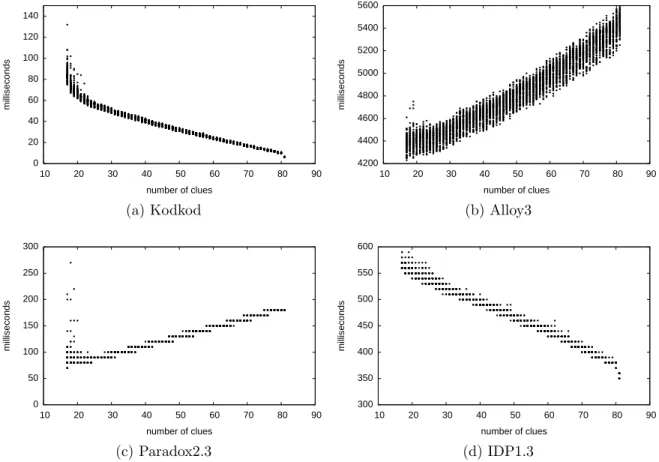
The impact of partial models on various model finders is observable even on small problems, like Sudoku. Figure 1-4, for example, shows the behavior of four state-of-the-art3 SAT-based model finders on a progression of 6600 Sudoku puzzles with different numbers of givens, or clues. The puzzle progression was constructed itera-tively from 100 original puzzles which were randomly selected from a public database of 17-clue Sudokus [110]. Each original puzzle was expanded into 66 variants, with each consecutive variant differing from its predecessor by an additional, randomly chosen clue. Using the formulations in Fig. 1-2 as templates, the puzzles were speci-fied in the input languages of Paradox2.3 (first order logic), IDP1.3 (first order logic with inductive definitions), Alloy3 (relational logic), and Kodkod (bounded relational logic). The data points on the plots in Fig. 1-4 represent the CPU time, in millisec-onds, taken by the model finders to discover the models of these specifications. All experiments were performed on a 2 × 3 GHz Dual-Core Intel Xeon with 2 GB of RAM. Alloy3, Paradox2.3, and Kodkod were configured with MiniSat [43] as their SAT solver, while IDP1.3 uses MiniSatID [89], an extension of MiniSat for proposi-tional logic with inductive definitions.
The performance of the traditional model finders, Alloy3 (Fig. 1-4b) and Para-dox2.3 (Fig. 1-4c), degrades steadily as the number of clues for each puzzle increases. On average, Alloy3 is 25% slower on a puzzle with a fully specified grid than on a puzzle with 17 clues, whereaes Paradox2.3 is twice as slow on a full grid. The per-formance of the model extenders (Figs. 1-4a and 1-4d), on the other hand, improves with the increasing number of clues. The average improvement of Kodkod is 14 times on a full grid, while that of IDP1.3 is about 1.5 times.
The trends in Fig. 1-4 present a fair picture of the relative performance of Kodkod and other SAT-based tools on a wide range of problems. Due to the new translation techniques described in Chapters 2-3, Kodkod is roughly an order of magnitude faster than Alloy3 with and without partial models. It is also faster than IDP1.3 and
Para-3With the exception of Alloy3, which has been superseded by a new version based on Kodkod,
0 20 40 60 80 100 120 140 10 20 30 40 50 60 70 80 90 milliseconds number of clues (a) Kodkod 4200 4400 4600 4800 5000 5200 5400 5600 10 20 30 40 50 60 70 80 90 milliseconds number of clues (b) Alloy3 0 50 100 150 200 250 300 10 20 30 40 50 60 70 80 90 milliseconds number of clues (c) Paradox2.3 300 350 400 450 500 550 600 10 20 30 40 50 60 70 80 90 milliseconds number of clues (d) IDP1.3
Figure 1-4: Effect of partial models on the performance of SAT-based model finders, when applied to a progression of 6600 Sudoku puzzles. The x-axis of each graph shows the number of clues in a puzzle, and the y-axis shows the time, in milliseconds, taken by a given model finder to solve a puzzle with the specified number of clues. Note that Paradox2.3, IDP1.3 and Kodkod solved many of the puzzles with the same number of clues in the same amount of time (or within a few milliseconds of one another), so many of the points on their performance graphs overlap.
0 50 100 150 200 250 300 10 20 30 40 50 60 70 80 90 milliseconds number of clues
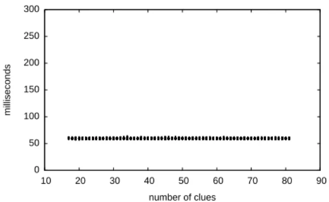
Figure 1-5: Effect of partial models on the performance of a dedicated Sudoku solver, when applied to a progression of 6600 Sudoku puzzles.
dox2.3 on the problems that this thesis targets—that is, specifications with partial models and intricate constraints over relational structures.4 For a potential user of
these tools, however, the interesting question is not necessarily how they compare to one another. Rather, the interesting practical question is how they might compare to a custom translation to SAT.
This question is hard to answer in general, but a comparison with existing cus-tom translations is promising. Figure 1-5, for example, shows the performance of a dedicated, SAT-based Sudoku solver on the same 6600 puzzles solved with Kodkod and the three other model finders. The solver consists of 150 lines of Java code that generate Lynce and Ouaknine’s optimized SAT encoding [86] of a given Sudoku puz-zle, followed by an invocation of MiniSat on the generated file. The program took a few hours to write and debug, as the description of the encoding [86] contained several errors and ambiguities that had to be resolved during implementation. The Kodkod-based solver, in contrast, consists of about 50 lines of Java API calls that directly correspond to the text in Fig. 1-2a; it took an hour to implement.
The performance of the two solvers, as Figs. 1-4a and 1-5 show, is comparable. The dedicated solver is slightly faster on 17-clue Sudokus, and the Kodkod solver is faster on full grids. The custom solver’s performance remains constant as the number of clues in each puzzle increases because it handles the additional clues by feeding extra unit clauses to the SAT solver: adding these clauses takes negligible
time, and, given that the translation time heavily dominates the SAT solving time, their positive effect on MiniSat’s performance is unobservable. Both implementations were also applied to 16 × 16 and 25 × 25 puzzles, with similar outcomes.5 The solvers
based on other model finders were unable to solve Sudokus larger than 16 × 16.
1.3
Minimal unsatisfiable core extraction
When a specification has no models in a given universe, most model finders [25, 51, 68, 70, 88, 91, 122, 151, 152] simply report that it is unsatisfiable in that universe and offer no further feedback. But many applications need to know the cause of a specification’s unsatisfiability, either to take corrective action (in the case of declar-ative configuration [133]) or to check that no models exist for the right reasons (in the case of bounded verification [31, 21]). A bounded verifier [31, 21], for example, checks a system description s1∧ . . . ∧ sn against a property p in some finite universe
by looking for models of the formula s1∧ . . . ∧ sn∧ ¬p in that universe. If found, such
a model, or a counterexample, represents a behavior of the system that violates p. A lack of models, however, does not necessarily mean that the analysis was successful. If no models exist because the system description is overconstrained, or because the property is a tautology, the analysis is considered to have failed due to a vacuity error. A cause of unsatisfiability of a given specification, expressed as a subset of the specification’s constraints that is itself unsatisfiable, is called an unsatisfiable core. Every unsatisfiable core includes one or more critical constraints that cannot be re-moved without making the remainder of the core satisfiable. Non-critical constraints, if any, are irrelevant to unsatisfiability and generally decrease a core’s utility both for diagnosing faulty configurations [133] and for checking the results of a bounded analysis [129]. Cores that include only critical constraints are said to be minimal.
5The bounded relational encoding of Sudoku used in these experiments (Fig. 1-2a) is the easiest
to understand, but it does not produce the most optimal SAT formulas. An alternative encoding, where the multiplicity some on line 10 is replaced by one and each constraint of the form ‘∀ x: ri,
y: rj | no (grid[x][y] ∩ grid[ri\x][rj\y])’ is loosened to ‘num ⊆ grid[ri][rj],’ actually produces a SAT
encoding that is more efficient than the custom translation across the board. For example, MiniSat solves the SAT formula corresponding to the alternative encoding of a 64 × 64 Sudoku ten times faster than the custom SAT encoding of the same puzzle.
3 8 2 4 1 9 6 1 8 9 3 5 6 9 1 3 9 7 3 5 8 1 9 8 9 4 5 6 3 5 6 4 2
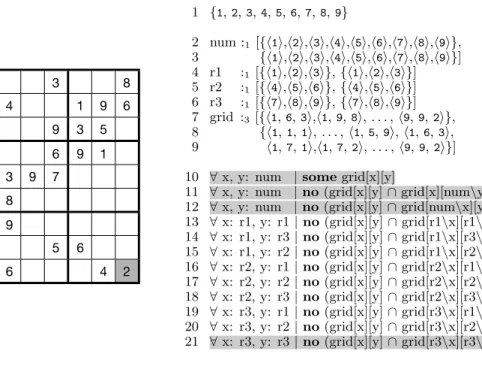
(a) An unsatisfiable Sudoku puzzle
1 {1,2,3,4,5,6,7,8,9} 2 num :1[{h1i,h2i,h3i,h4i,h5i,h6i,h7i,h8i,h9i}, 3 {h1i,h2i,h3i,h4i,h5i,h6i,h7i,h8i,h9i}] 4 r1 :1 [{h1i,h2i,h3i}, {h1i,h2i,h3i}] 5 r2 :1 [{h4i,h5i,h6i}, {h4i,h5i,h6i}] 6 r3 :1 [{h7i,h8i,h9i}, {h7i,h8i,h9i}]
7 grid :3 [{h1,6,3i,h1,9,8i, . . . , h9,9,2i},
8 {h1,1,1i, . . . , h1,5,9i, h1,6,3i, 9 h1,7,1i,h1,7,2i, . . . , h9,9,2i}] 10 ∀ x, y: num | some grid[x][y]
11 ∀ x, y: num | no (grid[x][y] ∩ grid[x][num\y]) 12 ∀ x, y: num | no (grid[x][y] ∩ grid[num\x][y]) 13 ∀ x: r1, y: r1 | no (grid[x][y] ∩ grid[r1\x][r1\y]) 14 ∀ x: r1, y: r3 | no (grid[x][y] ∩ grid[r1\x][r3\y]) 15 ∀ x: r1, y: r2 | no (grid[x][y] ∩ grid[r1\x][r2\y]) 16 ∀ x: r2, y: r1 | no (grid[x][y] ∩ grid[r2\x][r1\y]) 17 ∀ x: r2, y: r2 | no (grid[x][y] ∩ grid[r2\x][r2\y]) 18 ∀ x: r2, y: r3 | no (grid[x][y] ∩ grid[r2\x][r3\y]) 19 ∀ x: r3, y: r1 | no (grid[x][y] ∩ grid[r3\x][r1\y]) 20 ∀ x: r3, y: r2 | no (grid[x][y] ∩ grid[r3\x][r2\y]) 21 ∀ x: r3, y: r3 | no (grid[x][y] ∩ grid[r3\x][r3\y])
(b) Core of the puzzle (highlighted)
Figure 1-6: An unsatisfiable Sudoku puzzle and its core.
Figure 1-6 shows an example of using a minimal core to diagnose a faulty Sudoku configuration. The highlighted parts of Fig. 1-6b comprise a set of critical constraints that cannot be satisfied by the puzzle in Fig. 1-6a. The row (line 11) and column (line 12) constraints rule out ‘9’ as a valid value for any of the blank cells in the bottom right region. The values ‘2’, ‘4’, and ‘6’ are also ruled out (line 21), leaving five unique numbers and six empty cells. By the pigeonhole principle, these cells cannot be filled (as required by line 10) without repeating some value (which is disallowed by line 21). Removing ‘2’ from the highlighted cell fixes the puzzle.
The problem of unsatisfiable core extraction has been studied extensively in the SAT community, and there are many efficient algorithms for finding small or minimal cores of propositional formulas [32, 60, 61, 59, 79, 85, 97, 102, 153]. A simple facility for leveraging these algorithms in the context of SAT-based model finding has been implemented as a feature of Alloy3. The underlying mechanism [118] involves trans-lating a specification to a SAT problem; finding a core of the translation using an existing SAT-level algorithm [153]; and mapping the clauses from the boolean core
back to the specification constraints from which they were generated. The resulting specification-level core is guaranteed to be sound (i.e. unsatisfiable) [118], but it is not guaranteed to be minimal or even small.
Recycling core extraction (RCE) is a new SAT-based algorithm for finding cores of declarative specifications that are both sound and minimal. It has two key ideas (Chapter 4). The first idea is to lift the minimization process from the boolean level to the specification level. Instead of attempting to minimize the boolean core, RCE maps it back and then minimizes the resulting specification-level core, by removing candidate constraints and testing the remainder for satisfiability. The second idea is to use the proof of unsatisfiability returned by the SAT solver, and the mapping be-tween the specification constraints and the translation clauses, to identify the boolean clauses that were inferred by the solver and that still hold when a specification-level constraint is removed. By adding these clauses to the translation of a candidate core, RCE allows the solver to reuse previously made inferences.
Both ideas employed by RCE are straightforward and relatively easy to imple-ment, but have dramatic consequences on the quality of the results obtained and the performance of the analysis. Compared to NCE and SCE [129], two variants of RCE that lack some of its optimizations, RCE is roughly 20 to 30 times faster on hard problems and 10 to 60 percent faster on easier problems (Chapter 4). It is much slower than Alloy3’s core extractor, OCE [118], which does not guarantee minimal-ity. Most cores produced by OCE, however, include large proportions of irrelevant constraints, making them hard to use in practice.
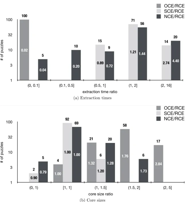
Figure 1-7, for example, compares RCE with OCE, NCE and SCE on a set of 100 unsatisfiable Sudokus. The puzzles were constructed from 100 randomly selected 16 × 16 Sudokus [63], each of which was augmented with a randomly chosen, faulty clue. Figure 1-7a shows the number of puzzles on which RCE is faster (or slower) than each competing algorithm by a factor that falls within the given range. Figure 1-7b shows the number of puzzles whose RCE cores are smaller (or larger) than those of the competing algorithms by a factor that falls within the given range. All four extractors were implemented in Kodkod, configured with MiniSat, and all experiments
1 3 10 32 100 (0, 0.1] (0.1, 0.5] (0.5, 1] (1, 2] (2, 16] 20 56 9 10 5 14 71 15 100 # of puzzles
extraction time ratio
OCE/RCE SCE/RCE NCE/RCE 0.20 0.04 0.72 0.02 0.89 1.21 1.44 2.74 4.40
(a) Extraction times
1 3 10 32 100 (0, 1) [1, 1] (1, 1.5] (1.5, 2] (2, 5] 6 20 69 5 6 92 2 17 58 21 4 # of puzzles
core size ratio
OCE/RCE SCE/RCE NCE/RCE 1.00 1.00 1.00 0.90 0.79 1.32 1.20 1.28 1.76 1.73 2.84 (b) Core sizes
Figure 1-7: Comparison of SAT-based core extractors on 100 unsatisfiable Sudokus. Figure (a) shows the number of puzzles on which RCE is faster, or slower, than each competing algorithm by a factor that falls within the given range. Figure (b) shows the number of puzzles whose RCE cores are smaller, or larger, than those of the competing algorithms by a factor that falls within the given range. Both histograms are shown on a logarithmic scale. The number above each column specifies its height, and the middle number is the average extraction time (or core size) ratio for the puzzles in the given category.
were performed on a 2 × 3 GHz Dual-Core Intel Xeon with 2 GB of RAM.
Because SCE is essentially RCE without the clause recycling optimization, they usually end up finding the same minimal core. Of the 100 cores extracted by each algorithm, 92 were the same (Fig. 1-7b). RCE was faster than SCE on 85 of the problems (Fig. 1-7a). Since Sudoku cores are easy to find6, the average speed up of
RCE over SCE is about 37%. NCE is the most naive of the three approaches and does not exploit the boolean-level cores in any way. It found a different minimal core than RCE for 31 of the puzzles. For 26 of those, the NCE core was larger than the RCE core, and indeed, easier to find, as shown in Fig. 1-7a. Nonetheless, RCE was, on average, 77% faster than NCE. OCE outperformed all three minimality-guaranteeing algorithms by large margins. However, only four OCE cores were minimal, and more than half the constraints in 75 of its cores were irrelevant.
1.4
Summary of contributions
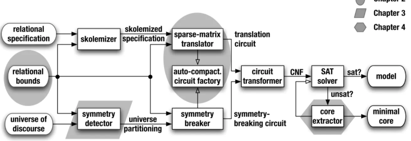
This thesis contributes a collection of techniques (Fig. 1-8) that enable easy and efficient use of SAT for declarative problem solving. They include:
1. A new problem-description language that extends the relational logic of Al-loy [69] with a mechanism for specifying precise bounds on the values of free variables (Chapter 2); the bounds enable efficient encoding and exploitation of partial models.
2. A new translation to SAT that uses sparse-matrices and auto-compacting cir-cuits (Chapter 2); the resulting boolean encoding is significantly smaller, faster to produce, and easier to solve than the encodings obtained with previously published techniques [40, 119].
3. A new algorithm for identifying symmetries that works in the presence of arbi-trary bounds on free variables (Chapter 3); the algorithm employs a fast greedy
6Chapter 4 describes a metric for approximating the difficulty of a given problem for a particular
relational specification relational bounds universe of discourse skolemizer symmetry
detector symmetrybreaker skolemized specification universe partitioning circuit transformer translation circuit symmetry-breaking circuit sparse-matrix translator SAT solver CNF model auto-compact.
circuit factory sat?
core extractor unsat? minimal core Chapter 3 Chapter 2 Chapter 4
Figure 1-8: Summary of contributions. The contributions of this thesis are highlighted with gray shading; the remaining parts of the framework are implemented using standard techniques. Filled arrows represent data and control flow between components. Clear arrows represent usage relationships between components.
technique that is both effective in practice and scales better than a complete method based on graph automorphism detection.
4. A new algorithm for finding minimal unsatisfiable cores that recycles infer-ences made at the boolean level to speed up core extraction at the specification level (Chapter 4); the algorithm is much faster on hard problems than related approaches [129], and its cores are much smaller than those obtained with non-minimal extractors [118].
These techniques have been prototyped in Kodkod, a new engine for finding mod-els and cores of large relational specifications. The engine significantly outperforms existing model finders [13, 25, 88, 93, 117, 152] on problems with partial models, rich type hierarchies, and low-arity relations. As such problems arise in a wide range of declarative configuration and analysis settings, Kodkod has been used in several configuration [149, 101], test-case generation [114, 135] and bounded verifi-cation [21, 137, 31, 126, 34] tools (Table 1.1). These appliverifi-cations have served as a comprehensive testbed for Kodkod, revealing both its strengths and limitations. The latter open up a number of promising directions for future work (Chapter 5).
b ound e d v er ificati on
Alloy4 [21] analyzer for the Alloy language. Alloy4 uses Kodkod for simulation and checking of software designs expressed in the Alloy modeling language. It is 2 to 10 times faster than Alloy3 and provides a precise debugger for overconstrained specifications that is based on Kodkod’s core extraction facility. Like its predecessor, Alloy4 has been used for modeling and analysis in a variety of contexts, e.g. filesystems [75], security [81], and requirements engineering [113].
Kato [136, 137] slicer for declarative specifications. Kato uses Kodkod to slice and solve Al-loy specifications of complex data structures, such as red-black trees and doubly-linked lists. The tool splits a given specification into base and derived constraints using a heuristically selected slicing criterion. The resulting slices are then fed to Kodkod separately so that a model of the base slice becomes a partial model for the derived slice. The final model, if any, satisfies the entire specification. Because the subproblems are usually easier to solve than the entire specification, Kato scales better than Alloy4 on specifications that are amenable to slicing.
Forge [30, 31], Karun [126], and Minatur [34] bounded code verifiers. These tools use Kodkod to check the methods of a Java class against rich structural properties. The basic analysis [138] involves encoding the behavior of a given method, within a bounded heap, as a set of relational constraints that are conjoined with the negation of the property being checked. A model of the resulting specification, if one exists, represents a concrete trace of the method that violates the property. All three tools have been used to find previously unknown bugs in open source systems, including a heavily tested job scheduler [126] and an electronic vote tallying system that had been already checked with a theorem prover [30].
test-cas e gener at ion
Kesit [134, 135] test-case generator for software product lines. Kesit uses Kodkod to in-crementally generate tests for products in a software product line. Given a product that is composed of a base and a set of features, Kesit first generates a test suite for the base by feeding a specification of its functionality to Kodkod. The tests from the resulting test-suite (derived from the models of the specification) are then used as partial models for the speci-fication of the features. Because the product is specified by the conjunction of the base and feature constraints, the final set of models is a valid test-suite for the product as a whole. Kesit’s approach to test-case generation has been shown to scale over 60 times better than previous approaches to specification-based testing [76, 77].
Whispec [114] test-case generator for white-box testing. Whispec uses Kodkod to generate white-box tests for methods that manipulate structurally complex data. To test a method, Whispec first obtains a model of the constraints that specify the method’s preconditions. The model is then converted to a test input, which is fed to the method. A path condition of the resulting execution is recorded, and new path conditions (for unexplored paths) are constructed by negating the branch predicates in the recorded path. Next, Kodkod is applied to the conjunction of the pre-condition and one of the new path conditions to obtain a new test input. This process is repeated until the desired level of code coverage is reached. Whispec has been shown to generate significantly smaller test suites, with better coverage, than previous approaches.
decl ar ati v e configuration
ConfigAssure [100, 101] system for network configuration. ConfigAssure uses Kodkod for synthesis, diagnosis and repair of network configurations. Given a partially configured net-work and set of configuration requirements, ConfigAssure generates a relational satisfiability problem that is fed to Kodkod. If a model is found, it is translated back to a set of configura-tion assignments: nodes to subnets, IP addresses to nodes, etc. Otherwise, the tool obtains an unsatisfiable core of the configuration formula and repairs the input configuration by removing the configuration assignments that are in the core. ConfigAssure has been shown to scale to realistic networks with hundreds of nodes and subnets.
A declarative course scheduler [148, 149]. The scheduler uses Kodkod to plan a student’s schedule based on the overall requirements and prerequisite dependencies of a degree pro-gram; courses taken so far; and the schedule according to which particular courses are offered. The scheduler is offered as a free, web-based service to MIT students. Its performance is competitive with that of conventional planners.
Chapter 2
From Relational to Boolean Logic
The relational logic of Alloy [69] combines the quantifiers of first order logic with the operators of relational algebra. The logic and the language were designed for modeling software abstractions, their properties and invariants. But unlike the logics of traditional modeling languages [123, 143], Alloy makes no distinction between relations, sets and scalars: sets are relations with one column, and scalars are singleton sets. Treating everything as a relation makes the logic more uniform and, in some ways, easier to use than traditional modeling languages. Applying a partial function outside of its domain, for example, simply yields the empty set, eliminating the need for special undefined values.
The generality and versatility of Alloy’s logic have prompted several attempts to use its model finder, Alloy3 [117], as a generic constraint solving engine for declarative configuration [99] and analysis [76, 138]. These efforts, however, were hampered by two key limitations of the Alloy system. First, Alloy has no notion of a partial model. If a partial solution, or a model, is available for a set of Alloy constraints, it can only be provided to the solver in the form of additional constraints. Because the solver is essentially forced to rediscover the partial model from the constraints, this strategy does not scale well in practice. Second, Alloy3 was designed for small-scope analysis [69] of hand-crafted specifications of software systems, so it performs poorly on problems with large universes or large, automatically generated specifications.
Its model finder, like Alloy3, works by translating relational to boolean logic and applying an off-the-shelf SAT solver to the resulting boolean formula. Unlike Alloy3, however, Kodkod scales in the presence of partial models, and it can handle large universes and specifications. This chapter describes the elements of Kodkod’s logic and model finder that are key to its ability to produce compact SAT formulas, with and without partial models. Next chapter describes a technique that is used for making the produced formulas slightly larger but easier to solve.
2.1
Bounded relational logic
A specification in the relational logic of Alloy is a collection of constraints on a set of relational variables. A model of an Alloy specification is a binding of its free variables to relational constants that makes the specification true. These constants are sets of tuples, drawn from a common universe of uninterpreted elements, or atoms. The universe itself is implicit, in the sense that its elements cannot be named or referenced through any syntactic construct of the logic. As a result, there is no direct way to specify relational constants in Alloy. If a partial binding of relations to constants— i.e. a partial model—is available for a specification, it must be encoded indirectly, with constraints that use additional variables (e.g. N1 through N9 in Fig. 1-2b) as implicit handles to distinct atoms. While sound, this encoding of partial models is impractical because the additional variables and constraints make the resulting model finding problem larger rather than smaller.
The bounded relational logic of Kodkod (Fig. 2-1) extends Alloy in two ways: the universe of atoms for a specification is made explicit, and the value of each free variable is explicitly bound, above and below, by relational constants. A problem description in Kodkod’s logic consists of an Alloy specification, augmented with a universe declaration and a set of bound declarations. The universe declaration specifies the set of atoms from which a model of the specification is to be drawn. The bound declarations bound the value of each relation with two relational constants drawn from the declared universe: an upper bound, which contains the tuples that the relation
problem := universe relBound∗formula∗ universe := { atom[, atom]∗}
relBound := var :arity[[constant, constant]]
constant := {tuple[, tuple]∗} | {}[×{}]∗
tuple := hatom[, atom]∗i atom, var := identifier arity := positive integer formula :=
no expr empty | lone expr at most one | one expr exactly one | some expr non-empty | expr ⊆ expr subset | expr = expr equal | ¬ formula negation | formula ∧ formula conjunction | formula ∨ formula disjunction | formula ⇒ formula implication | formula ⇔ formula equivalence | ∀ varDecls || formula universal | ∃ varDecls || formula existential expr :=
var variable
| ˜expr transpose | ˆexpr closure |∗expr reflex. closure
| expr ∪ expr union | expr ∩ expr intersection | expr \ expr difference | expr . expr join | expr → expr product | formula ? expr : expr if-then-else | {varDecls || formula} comprehension varDecls := var : expr[, var : expr]∗
(a) Abstract syntax
P : problem → binding → boolean R : relBound → binding → boolean F : formula → binding → boolean E : expr → binding → constant binding : var → constant
PJ{a1, . . . , an} r1. . . rj f1. . . fmKb := RJr1Kb ∧ . . . ∧ RJrjKb ∧ FJf1Kb ∧ . . . ∧ FJfmKb RJv :k[l, u]Kb := l ⊆ b(v) ⊆ u FJno pKb := |EJpKb| = 0 FJlone pKb := |EJpKb| ≤ 1 FJone pKb := |EJpKb| = 1 FJsome pKb := |EJpKb| > 0 FJp ⊆ qKb := EJpKb ⊆ EJqKb FJp = qKb := EJpKb = EJqKb FJ¬f Kb := ¬FJf Kb FJf ∧ gKb := FJf Kb ∧ FJgKb FJf ∨ gKb := FJf Kb ∨ FJgKb FJf ⇒ gKb := FJf Kb ⇒ FJgKb FJf ⇔ gKb := FJf Kb ⇔ FJgKb FJ∀ v1: e1, ..., vn: en|| fKb := V s∈EJe1Kb(FJ∀ v2: e2, ..., vn: en|| fK(b ⊕ v17→ {hsi}) FJ∃ v1: e1, ..., vn: en|| fKb := W s∈EJe1Kb(FJ∃ v2: e2, ..., vn: en|| fK(b ⊕ v17→ {hsi}) EJvKb := b(v) EJ˜pKb := {hp2, p1i | hp1, p2i ∈ EJpKb} EJˆpKb := {hp1, pni | ∃ p2, ..., pn−1| hp1, p2i, ..., hpn−1, pni ∈ EJpKb} EJ ∗p Kb := EJˆpKb ∪ {hp1, p1i | true} EJp ∪ qKb := EJpKb ∪ EJqKb EJp ∩ qKb := EJpKb ∩ EJqKb EJp \ qKb := EJpKb \ EJqKb EJp . qKb := {hp1, ..., pn−1, q2, ..., qmi | hp1, ..., pni ∈ EJpKb ∧ hq1, ..., qmi ∈ EJqKb } EJp → qKb := {hp1, ..., pn, q1, ..., qmi | hp1, ..., pni ∈ EJpKb ∧ hq1, ..., qmi ∈ EJqKb } EJf ? p : qKb := if FJf Kb then EJpKb else EJqKb EJ{v1: e1, ..., vn: en|| f }Kb := {hs1, ..., sni | s1∈ EJe1Kb ∧ s2∈ EJe2K(b ⊕ v17→ {hs1i}) ∧ . . . ∧ sn∈ EJenK(b ⊕ Sn−1 i=1 vi7→ {hsii}) ∧ FJf K(b ⊕Sn i=1vi7→ {hsii})} (b) Semantics
Figure 2-1: Syntax and semantics of bounded relational logic. Because Kodkod is designed as a Java API, the users communicate with it by constructing universes, bounds, and formulas via API calls. The syntax presented here is for illustrative purposes only. Mixed and zero arity expressions are not allowed. The arity of a relation is the same as the arity of its bounding constants. There is exactly one bound declaration v :k [l, u] for each relation
v that appears in a problem description. The empty set {} has arity 1. The empty set of arity k is represented by taking the cross product of the empty set with itself k times, i.e. {} × . . . × {}.
1 {d0, d1, f0, f1, f2}
2 File :1 [{}, {hf0i,hf1i,hf2i}]
3 Dir :1 [{}, {hd0i,hd1i}]
4 Root :1 [{hd0i}, {hd0i}]
5 contents :2 [{hd0, d1i},
{hd0, d0i, hd0, d1i, hd0, f0i, hd0, f1i, hd0, f2i, hd1, d0i, hd1, d1i, hd1, f0i, hd1, f1i, hd1, f2i}] 6 contents ⊆ Dir → (Dir ∪ File)
7 ∀ d: Dir || ¬(d ⊆ d.ˆcontents) 8 Root ⊆ Dir
9 (File ∪ Dir) ⊆ Root.∗contents
(a) Problem description
File 7→ {hf0i,hf1i} Dir 7→ {hd0i,hd1i} Root 7→ {hd0i}
contents 7→ {hd0, d1i, hd0, f0i, hd1, f1i} d0 d1 f0 f1 contents contents contents Root Dir File (b) A sample model
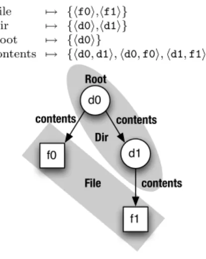
Figure 2-2: A toy filesystem.
may include, and a lower bound, which contains the tuples that the relation must include. Collectively, the lower bounds define a partial model, and the upper bounds limit the pool of values available for completing that partial model.
Figure 2-2a demonstrates the key features of Kodkod’s logic on a toy specification of a filesystem. The specification (lines 6-9) has four free variables: the binary relation contentsand the unary relationsFile,Dir, andRoot. File andDir represent the files and directories that make up the filesystem. The contents relation is an acyclic mapping of directories to their contents, which may be files or directories (line 6-7). Root represents the root of the filesystem: it is a directory (line 8) from which all files and directories are reachable by following thecontentsrelation zero or more times (line 9). The filesystem universe consists of five atoms (line 1). These are used to construct lower and upper bounds on the free variables (lines 2-5). The upper bounds on File and Dir partition the universe into atoms that represent directories (d0 and d1) and those that represent files (f0, f1, and f2); their lower bounds are empty. The Root relation has the same lower and upper bound, which ensures that all filesystem models found by Kodkod are rooted atd0. The bounds on thecontentsrelation specify that it must contain the tuple hd0,d1i and that its remaining tuples, if any, must be drawn from the cross product of the directory atoms with the entire universe.
as required by its bounds. The contentsrelation includes the sole tuple from its lower bound and two additional tuples from its upper bound. File and Dir consist of the file and directory atoms that are related by contents, as required by the specification (Fig. 2-2a, lines 6, 8 and 9).
2.2
Translating bounded relational logic to SAT
Using SAT to find a model of a relational problem involves several steps (Fig. 1-8): translation to boolean logic, symmetry breaking, transformation of the boolean for-mula to conjunctive normal form, and conversion of a boolean model, if one is found, to a model of the original problem. The last two steps implement standard transfor-mations [44, 68], but the first two use novel techniques which are discussed in this section and the next chapter.
2.2.1
Translation algorithm
Kodkod’s translation algorithm is based on the simple idea [68] that a relation over a finite universe can be represented as a matrix of boolean values. For example, a binary relation drawn from the universe {a0, . . . , an−1} can be encoded with an n × n
bit matrix that contains a 1 at the index [i, j] when the relation includes the tuple hai, aji. More generally, given a universe of n atoms, the collection of possible values
for a relational variable v :k [l, u] corresponds to a k-dimensional matrix m with
m[i1, . . . , ik] = 1 if hai1, . . . , aiki ∈ l, V(v, hai1, . . . , aiki) if hai1, . . . , aiki ∈ u \ l, 0 otherwise,
where i1, . . . , ik ∈ [0 . . n) and V maps its inputs to unique boolean variables. These
matrices can then be used in a bottom-up, compositional translation of the entire specification (Fig. 2-3): relational expressions are translated using matrix operations, and relational constraints are translated as boolean constraints over matrix entries.
Figure 2-4 illustrates the translation process on the constraint contents ⊆ Dir → (Dir∪File) from the filesystem specification (Fig. 2-2a, line 6). The constraint and
TP : problem → bool
TR : relBound → universe → matrix
TF : formula → env → bool
TE : expr → env → matrix
env : var → matrix
bool := 0 | 1 | boolVar | ¬ bool | bool ∧ bool | bool ∨ bool | bool ? bool : bool boolVar := identifier
idx := hint[, int]∗i
V : var → hatom[, atom]∗i → boolVar boolean variable for a given tuple in a relation
L M : matrix → {idx[, idx]
∗} set of all indices in a matrix
J K : matrix → int
int size of a matrix, (size of a dimension)number of dimensions
[ ] : matrix → idx → bool matrix value at a given index M : intint→ (idx → bool) → matrix
M(sd, f ) := new m ∈ matrix where
JmK = s
d∧ ∀ ~x ∈ {0, ..., s − 1}d, m[~x] = f (~x)
M : intint→ idx → matrix
M(sd, ~x) := M(sd, λ~y. if ~y = ~x then 1 else 0)
TP[{a1, . . . , an} v1:k1[l1, u1] . . . vj:kj[lj, uj] f1. . . fm] := TF[
Vm
i=1fi](∪ji=1vi7→ TR[vi:ki[li, ui], {a1, . . . , an}])
TR[v :k[l, u], {a1, . . . , an}] := M(nk, λhi1, ...iki. if hai1, . . . , aiki ∈ l then 1
else if hai1, . . . , aiki ∈ u \ l then V(v, hai1, . . . , aiki)
else 0) TF[no p]e := ¬TF[some p]e
TF[lone p]e := TF[no p]e ∨ TF[one p]e
TF[one p]e := let m ← TE[p]e inW~x∈LmM
m[~x] ∧ (V
~ y∈LmM\{~x}
¬m[~y]) TF[some p]e := let m ← TE[p]e inW~x∈LmMm[~x]
TF[p ⊆ q]e := let m ← (¬TE[p]e ∨ TE[q]e) inV~x∈LmMm[~x]
TF[p = q]e := TF[p ⊆ q]e ∧ TF[q ⊆ p]e
TF[not f ]e := ¬TF[f ]e
TF[f ∧ g]e := TF[f ]e ∧ TF[g]e
TF[f ∨ g]e := TF[f ]e ∨ TF[g]e
TF[f ⇒ g]e := ¬TF[f ]e ∨ TF[g]e
TF[f ⇔ g]e := (TF[f ]e ∧ TF[g]e) ∨ (¬TF[f ]e ∧ ¬TF[g]e)
TF[∀ v1: e1, ..., vn: en|| f ]e := let m ← TE[e1]e inVx∈LmM~ (¬m[~x] ∨ TF[∀ v2: e2, ..., vn: en|| f ](e ⊕ v17→ M(JmK, ~x))) TF[∃ v1: e1, ..., vn: en|| f ]e := let m ← TE[e1]e inWx∈LmM~ (m[~x] ∧ TF[∀ v2: e2, ..., vn: en|| f ](e ⊕ v17→ M(JmK, ~x))) TE[v]e := e(v)
TE[˜p]e := (TE[p]e)T
TE[ˆp]e := let m ← TE[p]e, sd←JmK, sq ← (λx.i. if i = s then x else let y ← sq(x, i ∗ 2) in y ∨ y · y) in sq(m, 1) TE[∗p]e := let m ← TE[ˆp]e, sd←JmK in m ∨ M(s
d, λhi
1, . . . , idi. if i1= i2∧ . . . ∧ i1= ikthen 1 else 0)
TE[p ∪ q]e := TE[p]e ∨ TE[q]e
TE[p ∩ q]e := TE[p]e ∧ TE[q]e
TE[p \ q]e := TE[p]e ∧ ¬TE[q]e
TE[p . q]e := TE[p]e · TE[q]e
TE[p → q]e := TE[p]e × TE[q]e
TE[f ? p : q]e := let mp← TE[p]e, mp← TE[q]e in M(JmpK, λ~x. TF[f ]e ? mp[~x] : mq[~x]) TE[{v1: e1, ..., vn: en|| f }]e := let m1← TE[e1]e, sd←Jm1K in
M(sn, λhi
1, . . . , ini. let m2← TE[e2](e ⊕ v17→ M(s, hi1i)), . . . ,
mn← TE[en](e ⊕ v17→ M(s, hi1i) ⊕ . . . ⊕ vn−17→ M(s, hin−1i)) in
m1[i1] ∧ . . . ∧ mn[in] ∧ TF[f ](e ⊕ v17→ M(s, hi1i) ⊕ . . . ⊕ vn7→ M(s, hini)))
its subexpressions are translated in an environment that binds each free variable to a matrix that represents its value. The bounds on a variable are used to populate its representation matrix as follows: lower bound tuples are represented with 1s in the corresponding matrix entries; tuples that are in the upper but not the lower bound are represented with fresh boolean variables; and tuples outside the upper bound are represented with 0s. Translation of the remaining expressions is straightforward. The union of DirandFileis translated as the disjunction of their translations so that a tuple is in Dir∪File if it is in Dir or File; relational cross product becomes the generalized cross product of matrices, with conjunction used instead of multiplication; and the subset constraint forces each boolean variable representing a tuple inDir→ (Dir∪File) to evaluate to 1 whenever the boolean representation of the corresponding tuple in the contents relation evaluates to the same.
2.2.2
Sparse-matrix representation of relations
Many problems suitable for solving with a relational engine are typed: their uni-verses are partitioned into sets of atoms according to a type hierarchy, and their expressions are bounded above by relations over these sets [39]. The toy filesys-tem, for example, is defined over a universe that consists of two types of atoms: the atoms that represent directories and those that represent files. Each expres-sion in the filesystem specification (Fig. 2-2a) is bounded above by a relation over the types Tdir = {d0,d1} and Tfile = {f0,f1,f2}. The upper bound on contents,
for example, relates the directory type to both the directory and file types, i.e. dcontentse = {hTdir, Tdiri, hTdir, Tfilei} = {d0,d1} × {d0,d1} ∪ {d0,d1} × {f0,f1,f2}.
Previous relational engines (§2.3.1) employed a type checker [39, 128], a source-to-source transformation [40], and a typed translation [68, 117], in an effort to reduce the number of boolean variables used to encode typed problems. Kodkod’s translation, on the other hand, is designed to exploit types, provided as upper bounds on free variables, transparently: each relational variable is represented as an untyped matrix whose dimensions correspond to the entire universe, but the entries outside the vari-able’s upper bound are zeroed out. The zeros are then propagated up the translation
e = 8 > > > < > > > : File 7→ 2 6 6 6 4 0 0 f0 f1 f2 3 7 7 7 5 , Dir 7→ 2 6 6 6 4 d0 d1 0 0 0 3 7 7 7 5 , Root 7→ 2 6 6 6 4 1 0 0 0 0 3 7 7 7 5 , contents 7→ 2 6 6 6 4 c0 1 c2 c3 c4 c5 c6 c7 c8 c9 0 0 0 0 0 0 0 0 0 0 0 0 0 0 0 3 7 7 7 5 9 > > > = > > > ; . TE[Dir]e = e(Dir) = 2 6 6 6 4 d0 d1 0 0 0 3 7 7 7 5 , TE[File]e = e(File) = 2 6 6 6 4 0 0 f0 f1 f2 3 7 7 7 5 , TE[contents]e = e(contents) = 2 6 6 6 4 c0 1 c2 c3 c4 c5 c6 c7 c8 c9 0 0 0 0 0 0 0 0 0 0 0 0 0 0 0 3 7 7 7 5 .
TE[Dir ∪ File]e = TE[Dir]e ∨ TE[File]e =
2 6 6 6 4 d0 d1 0 0 0 3 7 7 7 5 ∨ 2 6 6 6 4 0 0 f0 f1 f2 3 7 7 7 5 = 2 6 6 6 4 d0 d1 f0 f1 f2 3 7 7 7 5 .
TE[Dir → (Dir ∪ File)]e = TE[Dir]e × TE[Dir ∪ File]e =
ˆ d0 d1 0 0 0 ˜ × 2 6 6 6 4 d0 d1 f0 f1 f2 3 7 7 7 5 = 2 6 6 6 4 d0∧ d0 d0∧ d1 d0∧ f0 d0∧ f1 d0∧ f2 d1∧ d0 d1∧ d1 d1∧ f0 d1∧ f1 d1∧ f2 0 0 0 0 0 0 0 0 0 0 0 0 0 0 0 3 7 7 7 5 .
TF[contents ⊆ Dir → (Dir ∪ File)]e =V( ¬ TE[contents]e ∨ TE[Dir → (Dir ∪ File)]e)
=V 0 B B B @ ¬ 2 6 6 6 4 c0 1 c2 c3 c4 c5 c6 c7 c8 c9 0 0 0 0 0 0 0 0 0 0 0 0 0 0 0 3 7 7 7 5 ∨ 2 6 6 6 4 d0∧ d0 d0∧ d1 d0∧ f0 d0∧ f1 d0∧ f2 d1∧ d0 d1∧ d1 d1∧ f0 d1∧ f1 d1∧ f2 0 0 0 0 0 0 0 0 0 0 0 0 0 0 0 3 7 7 7 5 1 C C C A =V 2 6 6 6 4 ¬c0∨(d0∧d0) ¬1∨(d0∧d1) ¬c2∨(d0∧f0) ¬c3∨(d0∧f1) ¬c4∨(d0∧f2) ¬c5∨(d1∧d0) ¬c6∨(d1∧d1) ¬c7∨(d1∧f0) ¬c8∨(d1∧f1) ¬c9∨(d1∧f2) 0 0 0 0 0 0 0 0 0 0 0 0 0 0 0 3 7 7 7 5 = (¬c0∨(d0∧d0))∧(¬1∨( d0∧d1))∧(¬c2∨(d0∧f0))∧(¬c3∨(d0∧f1))∧(¬c4∨(d0∧f2)) ∧ (¬c5∨( d1∧d0))∧(¬c6∨(d1∧d1))∧(¬c7∨(d1∧f0))∧(¬c8∨(d1∧f1))∧(¬c9∨(d1∧f2)).
Figure 2-4: A sample translation. The shading highlights the redundancies in the boolean encoding.
0 0 f0 f1 f2 = 3 f1 4 f2 2 f0 (a) TE[File]e c0 1 c2 c3 c4 c5 c6 c7 c8 c9 0 0 0 0 0 0 0 0 0 0 0 0 0 0 0 = 2 c2 3 c3 1 1 0 c0 4 c4 7 c7 8 c8 6 c6 5 c5 9 c9 (b) TE[contents]e
Figure 2-5: Sparse representation of the translation matrices TE[File]e and TE[contents]e
from Fig. 2-4. The upper half of each tree node holds its key, and the lower half holds its value. Matrices are indexed starting at 0.
chain, ensuring that no boolean variables are wasted on tuples guaranteed to be out-side an expression’s valuation. The upper bound on the expression Dir→ (Dir∪File), for example, is {hTdir, Tdiri, hTdir, Tfilei}, and the regions of its translation matrix (Fig.
2-4) that correspond to the tuples outside of its ‘type’ are zeroed out.
This simple scheme for exploiting both types and partial models is enabled by a new multidimensional sparse-matrix data structure for representing relations. As noted in previous work [40], an untyped translation algorithm cannot scale if based on the standard encoding of matrices as multi-dimensional arrays, because the number of zeros in a k-dimensional matrix over a universe of n atoms grows proportionally to nk. Kodkod therefore encodes translation matrices as balanced trees that store only non-zero values. In particular, each tree node corresponds to a non-zero cell (or a range of cells) in the full nk matrix. The cell at the index [i1, . . . , ik] that stores
the value v becomes a node with Pk
j=1ijn
k−j as its key and v as its value, where
the index-to-key conversion yields the decimal representation of the n-ary number i1. . . ik. Nodes with consecutive keys that store a 1 are merged into a single node
with a range of keys, enabling compact representation of lower bounds.
Figure 2-5 shows the sparse representation of the translation matrices TE[File]e
and TE[contents]e from Fig. 2-4. The File tree contains three nodes, with keys that
tree consists of ten nodes, each of which corresponds to a non-empty entry [i, j] in thecontentsmatrix, with i ∗ 5 + j as its key and the contents of [i, j] as its value. Both of the trees contain only nodes that represent exactly one cell in the corresponding matrix. It is easy to see, however, that the nodes 1 through 3 in the contents tree, for example, could be collapsed into a single node with [1 . . 3] as its key and 1 as its value if the entries [0, 2] and [0, 3] of the matrix were replaced with 1s.
Operations on the sparse matrices are implemented in a straightforward way, so that the cost of each operation depends on the number of non-zero entries in the ma-trix and the tree insertion, deletion, and lookup times. For instance, the disjunction of two matrices with m1 and m2 non-zero entries takes O((m1+ m2) log(m1 + m2))
time. It is computed simply by creating an empty matrix with the same dimensions as the operands; iterating over the operands’ nodes in the increasing order of keys; com-puting the disjunction of the values with matching keys; and storing the result, under the same key, in the newly created matrix. A value with an unmatched key is inserted directly into the output matrix (under its key), since the absence of a key from one of the operands is interpreted as its mapping that key to zero. Implementation of other operations follows the same basic idea.
2.2.3
Sharing detection at the boolean level
Relational specifications are typically built out of expressions and constraints whose boolean encodings contain many equivalent subcomponents. The expression Dir → (Dir∪File), for example, translates to a matrix that contains two entries with equiva-lent but syntactically distinct formulas: d0∧d1at index [0, 1] and d1∧d0 at index [1, 0]
(Fig. 2-4). The two formulas are propagated up to the translation of the enclosing constraint and, eventually, the entire specification, bloating the final SAT encoding and creating unnecessary work for the SAT solver. Detecting and eliminating struc-tural redundancies is therefore crucial for scalable model finding.
Prior work (§2.3.2) on redundancy detection for relational model finding produced a scheme that captures a class of redundancies detectable at the problem level. This class is relatively small and does not include the kind of low-level redundancy
![Figure 1-1: A hard Sudoku puzzle [58].](https://thumb-eu.123doks.com/thumbv2/123doknet/14461095.520459/13.918.352.568.676.892/figure-a-hard-sudoku-puzzle.webp)