HAL Id: halshs-01622466
https://halshs.archives-ouvertes.fr/halshs-01622466
Preprint submitted on 24 Oct 2017
HAL is a multi-disciplinary open access
archive for the deposit and dissemination of
sci-entific research documents, whether they are
pub-lished or not. The documents may come from
teaching and research institutions in France or
abroad, or from public or private research centers.
L’archive ouverte pluridisciplinaire HAL, est
destinée au dépôt et à la diffusion de documents
scientifiques de niveau recherche, publiés ou non,
émanant des établissements d’enseignement et de
recherche français ou étrangers, des laboratoires
publics ou privés.
Behavioral Uncertainty and the dynamics of traders’
confidence in their Price forecasts
Nobuyuki Hanaki, Eizo Akiyama, Ryuichiro Ishikawa
To cite this version:
Nobuyuki Hanaki, Eizo Akiyama, Ryuichiro Ishikawa. Behavioral Uncertainty and the dynamics of
traders’ confidence in their Price forecasts . 2017. �halshs-01622466�
Behavioral Uncertainty and the
dynamics of traders’ confidence in
their Price forecasts
Documents de travail GREDEG
GREDEG Working Papers Series
Nobuyuki Hanaki
Eizo Akiyama
Ryuichiro Ishikawa
GREDEG WP No. 2017-18
https://ideas.repec.org/s/gre/wpaper.html
Les opinions exprimées dans la série des Documents de travail GREDEG sont celles des auteurs et ne reflèlent pas nécessairement celles de l’institution. Les documents n’ont pas été soumis à un rapport formel et sont donc inclus dans cette série pour obtenir des commentaires et encourager la discussion. Les droits sur les documents appartiennent aux auteurs.
Behavioral uncertainty and the dynamics of traders’
confidence in their price forecasts
∗
Nobuyuki Hanaki
†Eizo Akiyama
‡Ryuichiro Ishikawa
§GREDEG Working Paper No. 2017-18
Abstract
By how much does the presence of behavioral uncertainty in an experimental asset market reduce subjects’ confidence in their price forecasts? An incentivized interval forecast elicitation method is employed to answer this question. Each market consists of six traders, and the value of dividends is known. Two treatments are considered: six human traders (6H), and one human interacting with five computer traders whose behavior is known (1H5C). We find that while the deviation of the initial price forecasts from the fundamental value is significantly smaller in the 1H5C treatment than in the 6H treatment, the average confidence regarding the forecasts is not. We further analyze the relationships between subjects’ confidence in their forecasts and their trading behavior, as well as their trading performance, in the 6H treatment. While subjects’ high confidence in their short-term forecasts shows a negative correlation with their trading performance, high confidence in their long-term forecasts shows a positive correlation with trading performance.
Keywords: Price forecasts, interval elicitation, experimental asset markets, behavioral uncertainty JEL Code: C90, D84
∗Makoto Soga provided invaluable help in organizing the experiments. This project is partly financed by L’Institute Universitaire de France, by JSPS KAKENHI Grant Numbers 26285043, 26350415, 26245026, and 26590026, by ANR ORA-Plus project “BEAM” (ANR-15-ORAR-0004), and by a grant-in-aid from the Zengin Foundation for Studies on Economics and Finance. The authors declare no conflict of interest associated with this manuscript. The experiments reported in this paper have been approved by the Institutional Review Board of the Faculty of Engineering, Information and Systems, University of Tsukuba (No. 2012R25-1).
†Universit´e Cˆote d’Azur, CNRS, GREDEG, France. Corresponding author. GREDEG, 250 rue Albert Einstein, 06560 Valbonne, FRANCE. E-mail: [email protected]
‡Faculty of Engineering, Information and Systems, University of Tsukuba. E-mail: [email protected] §School of International Liberal Studies, Waseda University. E-mail: [email protected]
1
Introduction
By how much does the presence of behavioral uncertainty reduce subjects’ confidence in their price forecasts? We aim to answer this question by employing an interval forecast elicitation method (Schlag and van der Weele, 2013) using the framework of Akiyama et al. (2017), who studied the effect of uncertainty about other traders’ behavior (behavioral uncertainty) on the initial deviation of price forecasts from fundamental value (FV) in an experimental asset market a la Smith et al. (1988).
The interval forecast elicitation method allows us to measure the confidence subjects have in each of their forecasts by asking subjects to submit ranges (between 0% and 19% in our study) around their forecasts within which they believe future prices will fall. The process is incentivized in that the narrower the range submitted, the higher the reward when the future prices fall within the range specified.
As Palan (2013) notes, despite the large body of literature employing the experimental framework of Smith et al. (1988), there is only a limited number of studies investigating the dynamics of forecasts (Haruvy et al., 2007; Akiyama et al., 2014, 2017; Bosch-Rosa et al., 2015; Eckel and F¨ullbrunn, 2015) or the relationship between the dynamics of forecasts, trading behavior, and market outcomes (Carle et al., 2015) despite the fact that the possibility of directly eliciting price forecasts from market participants is one of the great advantages of laboratory experiments.
Further, existing studies investigating forecast dynamics do not measure the degree of confidence market participants place in their price forecasts. We believe that measuring the degree of con-fidence will add additional insights because, as Scheinkman and Xiong (2003) show theoretically, heterogeneity among subjects regarding their confidence in their ability to forecast future prices can be an important source of speculative bubbles that are accompanied by large trading volumes and high price volatility. Odean (1998) also demonstrates theoretically that overconfident traders trade more and obtain lower expected payoffs than they would if they were not overconfident.
Such theoretical predictions are supported by Biais et al. (2005), Deaves et al. (2009), and Michailova and Schmidt (2016) who study the relationship between subjects’ degree of “overconfi-dence” (or “miscalibration,” to be more precise), their performance, and the degree of mispricing observed in the markets. These studies measure subjects’ degree of “overconfidence” based on a psychological test that asks subjects to answer multiple questions by providing an interval in
re-sponse to each question such that they are 90% sure that the correct answer will fall within the interval (Russo and Schowmaker, 1991), and then correlate their performance with (or in the case of Michailova and Schmidt (2016), construct a market based on) the measured degree of miscalibration. However, these studies do not directly measure the confidence subjects have in their price forecasts within asset markets.
To the best of our knowledge, one exception is Kirchler and Maciejovsky (2002). Their study measures the degree of subjects’ confidence in their price forecasts by eliciting, at the beginning of each period (a) an interval (high and low forecasts) within which subjects believe the current period price will fall with 98% likelihood, and (b) their subjective degree of confidence regarding the accuracy of their forecasts (on a nine-point scale ranging from not certain to certain). The results show that subjects tend to do poorly in calibrating their forecast intervals (the realized prices are outside the stated interval in more than 30% of cases), and their subjective degree of confidence tends to do well in capturing the accuracy of their forecasts. However, it should be noted that subjects were not provided with any monetary incentive in relation to their forecasting performance. Our study takes an additional step forward in that our interval forecast elicitation method is incentivized so that subjects who are more confident in the accuracy of their forecasts will submit narrower forecast ranges. We elicit both forecasts and their ranges in each period, which allows us to observe the dynamics of forecasts, confidence levels, trading behavior, and market outcomes. As the first step toward such a rich set of analyses, we investigate how much subjects’ confidence in their forecasts is affected by the presence of behavioral uncertainty, as well as how it evolves in two clearly distinct realizations of price dynamics.
Our results show that while eliminating behavioral uncertainty makes the initial forecasts of our subjects closer to the FV of the asset, it does not significantly increase our subjects’ confidence in their initial price forecasts. It is only after subjects have observed prices following a deterministic path for a few periods that their confidence in their price forecasts begins to increase significantly.
We further analyze the relationships between subjects’ confidence in their forecasts and (a) the dynamics of forecast adjustment, (b) trading behavior, and (c) trading performance. We find that when subjects have a high level of confidence in their forecasts, at least in the first round in which they participate, they tend to react less to the gap between their forecasts and observed prices, and raise their bids more when they expect a greater price increase in future periods. While trading performance is negatively correlated with subjects’ confidence in their short-term forecasts, it is
positively correlated with their confidence in their long-term forecasts.
The rest of the paper is organized as follows. Section 2 describes the experimental design, the results are presented in Section 3, and Section 4 concludes.
2
Experiment
We consider asset market experiments, a la Smith et al. (1988), with interval forecast elicitation (Schlag and van der Weele, 2013). Below, we explain the market environment, the interval forecast elicitation method we use, and the set of treatments we consider.
2.1
Markets
In both of the treatments, a group of six traders trades an asset with a life of 10 periods. All of the traders receive four units of an asset and 520 experimental currency units (ECUs) as their initial endowment. Each unit of the asset pays a dividend of 12 ECUs at the end of each period. After the final dividend payment in period 10, the asset loses its value. Therefore, the FV of the asset at the beginning of period t, F Vt, is 12(11 − t) ECUs. Note that we have eliminated the
uncertainty associated with dividend payments in each period because we are interested in the effect of uncertainty about others’ behavior on traders’ confidence in their forecasts.
We employ a call market structure for trading among subjects as in van Boening et al. (1993), Haruvy et al. (2007), Akiyama et al. (2014), Akiyama et al. (2017), and Bosch-Rosa et al. (2015). In call markets, unlike in continuous double auctions, there is one market clearing price for the asset in each period. Having only one price per period is advantageous for experiments with future price forecasts because the future prices to be forecasted are defined very clearly.1
In our call market experiment, subjects can submit a buy order as well as a sell order in each period by separately specifying a price and quantity for each type of order. Therefore, if subject i decides to submit a buy order in period t, he must specify the maximum price at which he is willing to buy a unit of the asset (bi
t, for bid) and the maximum number of units that he is willing to buy (dit)
in that period. Similarly, to submit a sell order in period t, a subject has to specify the minimum price at which he is willing to sell a unit of the asset (ai
t, for ask) and the maximum number of
units he is willing to sell (si
t) in that period. Of course, subjects can decide to submit neither a
buy order nor a sell order by setting the quantities in both types of order to zero. We impose three constraints on the orders subjects can submit: the admissible price range, a budget constraint, and the relationship between bit and ait in the case where a subject submits both buy and sell orders.
The admissible price range is set such that when dit≥ 1 (sit≥ 1), bit(ait) must be an integer between
1 and 2000, i.e., bi
t ∈ {1, 2, ..., 2000} (ait ∈ {1, 2, ..., 2000}). The budget constraint simply means
that neither borrowing of cash nor short-selling is allowed.2 The final constraint means that when a
trader submits both buy and sell orders, the ask price has to be no less than the bid price, ai t≥ bit.
We imposed a 60-second, non-binding time limit for submission of orders. When the time limit was reached, the subjects were told, via a message flashing in the upper right corner of their screen, to submit their orders as soon as possible.
Once all of the traders in the market have submitted their orders, the price that clears the market is calculated,3 and all transactions are processed at that price among traders who submitted a bid no less than, or an ask no greater than, the market clearing price.4
2.2
Interval forecast elicitation
In addition to trading units of an asset in a call market, at the beginning of each period (i.e., prior to submitting their orders), subjects are asked to submit price forecasts for each of the remaining periods, as well as the ranges ({0%, 1%, ..., 19%}) within which they think the market prices will fall.
That is, in period t, subject i submits 11 − t forecasts, ft,ki , for period k prices, pk, k ∈ {t, ..., 10},
and 11 − t corresponding ranges, wi
t,k ∈ {0, 1, ..., 19} (in percentage terms) around their forecasts.
Subjects obtained bonus points of (20 − wi
t,k), when pk was pk ∈ [(1 − wt,ki /100.)f i t,k, (1 + w i t,k/100.)f i t,k]
As can easily be seen, wider forecast ranges were penalized in that they generated lower bonus points.
2Thus, the budget constraint implies (i) di
t× bit ≤ cash holding at the beginning of the period, and (ii) sit ≤ units of the asset on hand at the beginning of the period.
3Following the design of Haruvy et al. (2007), when there are several such prices, the lowest price is chosen as the market clearing price. This is important because it ensures that the price does not spike upward in the absence of transactions at the market clearing price.
4Any ties among the last accepted buy or sell orders are resolved randomly. It is possible that no transactions take place given the computed market clearing price.
The bonus points for all 55 price forecasts over the 10 periods were summed.5 Let Bibe the total
number of points subject i obtained over 10 periods. Subjects were rewarded for their forecasting performance with a bonus payment in addition to what they obtained from their trading performance as follows:
Bonus (in ECUs) = 0.05% × Bi× cash holding after period 10.
For example if wi
t,k = 0 for all t and k, and the realized prices in all 10 periods were equal to
the forecast prices fi
t,k for all t and k, the subject received 20 × 55 = 1100 points. As a result, the
subject received an additional 55% of his cash holding at the end of period 10 as a bonus.
We imposed a 20 × (11 − t)-second, non-binding time limit for submission of price forecasts in period t. When the time limit was reached, the subjects were told, via a message flashing in the upper right corner of their screen, to submit their forecasts as soon as possible.
2.3
Treatments
We consider two treatments: one in which all six traders in a market are humans, and another in which only one of the six traders in a market is a human and the remaining five are computerized traders. We call the former treatment 6H and the latter treatment 1H5C.
All of the computerized traders in the 1H5C treatment behave in the following manner. In each period, they submit both buy and sell orders under the budget constraint restriction by setting bt= at= F Vt.
The behavior of the computerized traders is explained to subjects in the 1H5C treatment, but not to those in the 6H treatment.6 Thus, subjects in the 1H5C treatment do not face any uncertainty
regarding the behavior of other traders in the market, while those in the 6H treatment do.
Akiyama et al. (2017) employ the same framework except that they do not elicit the forecast range. The reward for forecast (fi
t,k) is based on the number of forecasts (out of the 55 that a subject
submits) that are within 10% of the realized price, that is, they receive a bonus equivalent to 0.5% of their final cash holding if their forecast price for period k, pk, is 0.9pk ≤ ft,ki ≤ 1.1pk.
Akiyama et al. (2017) found that the 10 initial forecasts submitted by subjects participating in 5Because subjects are making 11-t forecasts at the beginning of period t, they make a total of 55 forecasts during the 10 periods.
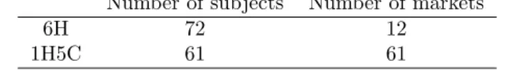
Table 1: Number of subjects and markets in the two treatments Number of subjects Number of markets
6H 72 12
1H5C 61 61
the 1H5C treatment deviated significantly less from FV than those submitted by subjects in the 6H treatment, suggesting that the presence of behavioral uncertainty has a significant effect on subjects’ expectations of market prices. They also found that while the observed differences in the deviations of the initial forecasts from FV between the two treatments were significantly positive for those subjects who scored highly in the cognitive reflection test (CRT, Frederick, 2005), this was not the case for those with very low CRT scores (0 or 1).
Building upon the finding of Akiyama et al. (2017), we are interested in comparing the confidence our subjects have in their forecasts (measured by wi
t,k) in the two treatments. All subjects repeated
the experiment in the same group of traders with the same initial endowment and the same dividend payments, i.e., subjects participated in two rounds of 10 periods each. They were paid the sum of their final cash holding from trading and receipt of dividends, as well as bonuses from the two rounds in which they participated.
3
Results
The experiments were conducted at the University of Tsukuba between January and July 2016.7 A
total of 133 subjects, 72 in the 6H treatment and 61 in the 1H5C treatment, participated in the experiment. These subjects had never participated in similar experiments, and they participated exclusively in one of the two treatments. Table 1 summarizes the number of subjects participating as well as the number of markets (six subjects per market in the 6H treatment and 1 subject per market in the 1H5C treatment) in the two treatments.
3.1
Initial forecasts and their deviations from FV
We follow Akiyama et al. (2017) in measuring the magnitude of the deviations of forecasts submitted by subject i in market m in period t from FV by the relative absolute forecast deviation (RAF Dti,m),
RAF Di,m1 wi,m1 0.0 0.5 1.0 1.5 2.0 2.5 3.0RAFD 0.0 0.2 0.4 0.6 0.8 1.0 CDF 0 5 10 15 20<w> 0.0 0.2 0.4 0.6 0.8 1.0 CDF p = 0.069 p = 0.388
Figure 1: Cumulative distribution of RAF D1 (left) and w1(right) in 6H (solid red line) and 1H5C
treatment (dashed blue line) groups in period 1 of Round 1. P-values are from the Mann–Whitney test (one-tailed).
which is defined as:
RAFDi,mt = 1 T − t + 1 T X k=t |ft,ki,m− F Vk| |F V | ,
where ft,ki,mis the forecast asset price in period k submitted by subject i in market m at the beginning of period t.8
We also consider the average forecast range submitted by subject i in market m in period t, wi,mt :
wi,mt = PT k=tw i,m t,k T − t + 1 .
Figure 1 shows the cumulative distribution of the initial forecast deviations, RAF D1i,m (left) and the initial average forecast range, wi,m1 (right) in Round 1 for 6H (solid red line) and 1H5C treatment (dashed blue line). Based on the findings of Akiyama et al. (2017), we expect RAF D1i,m in the 1H5C treatment to be smaller than that in the 6H treatment. We also expect that, given that subjects are informed about the behavior of the five computer traders in the market, wi,m1 in the 1H5C treatment will be smaller than that in the 6H treatment.
As expected, the distribution of RAF Di,m1 for the 1H5C treatment, shown in the left panel of Figure 1, lies to the left of that for the 6H treatment. The difference is statistically significant at the 10% level according to the one-tailed Mann–Whitney test (p = 0.069). However, our data show that the median average forecast range wi,m1 is the same for both the 1H5C and 6H treatment 8For clarity of exposition, we omit super/subscripts indicating the round. In the exposition below, we show results from two rounds of the experiment separately.
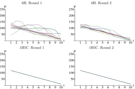
6H. Round 1 6H. Round 2 1 2 3 4 5 6 7 8 9 10t 50 100 150 200 250 P 1 2 3 4 5 6 7 8 9 10t 50 100 150 200 250 P 1H5C. Round 1 1H5C. Round 2 1 2 3 4 5 6 7 8 9 10t 50 100 150 200 250 P 1 2 3 4 5 6 7 8 9 10t 50 100 150 200 250 P
Figure 2: Price dynamics over two rounds in the 6H treatment (top) and 1H5C treatment (bottom).
(p = 0.388). It seems that subjects in the 1H5C treatment, while forecasting prices closer to FV than those in the 6H treatment, are initially no more confident in their forecasts than subjects in the 6H treatment. We now turn to the dynamics of forecast deviations and confidence.
3.2
Dynamics of forecast deviations and confidence
It is useful to review the price dynamics before discussing the forecast dynamics, because exist-ing studies demonstrate that forecasts tend to be adaptive (see, for example, Haruvy et al., 2007; Akiyama et al., 2014).
Figure 2 shows the dynamics of realized prices in Round 1 (left) and Round 2 (right) in the 6H treatment (top) and 1H5C treatment (bottom). Not surprisingly, given the way our computer traders behave, the prices in the 1H5C treatment follow FV, while the prices in the 6H treatment deviate from FV, with smaller deviations in Round 2 than in Round 1. We are interested in investigating how this difference in the price dynamics between the two treatments influences the dynamics of forecasts and confidence.
Because six subjects in the same market are observing the same realized prices before updating their price forecasts in the 6H treatment, their forecasts are not independent. For the analyses
Median RAF Dm t Round 1 Round 2 1 2 3 4 5 6 7 8 9 10t 0.5 1.0 1.5 2.0 RAFD 1 2 3 4 5 6 7 8 9 10t 0.0 0.5 1.0 1.5 2.0 RAFD Median wmt Round 1 Round 2 1 2 3 4 5 6 7 8 9 10t 0 5 10 15 20<w> 1 2 3 4 5 6 7 8 9 10t 0 5 10 15 20<w>
Figure 3: Dynamics of the median RAF Dtm(top) and wmt (bottom) in the 6H (solid red line) and 1H5C (dashed blue line) treatments over two rounds.
below, we take an average of RAF Dti,m, as well as wi,mt , across traders within a market to compute the average RAF Dm
t and wmt for price forecasts and ranges submitted by traders in period t in
market m. Below, we use this within-market average (across subjects in a market) as an independent observation.
Figure 3 shows the dynamics of the median RAF Dm
t (top) and w m
t (bottom) for the 6H (solid
red line) and 1H5C (dashed blue line) treatments over two rounds. Note that the median of the within-market average is plotted.
As noted above, the median RAF Dmis smaller in the 1H5C treatment than in the 6H treatment
in period 1 of Round 1. We also observe that the median RAF Dms rapidly declines in both the
1H5C and 6H treatments in the first couple of periods in Round 1. The median RAF Dm in the
1H5C treatment becomes zero by period 5 of Round 1 and remains there until the end of Round 2. The median RAF Dmin the 6H treatment remains positive, except for the last couple of periods in
Round 2, reflecting the deviations from FV of the observed prices in the 6H markets.
Conversely, the median wm in period 1 of Round 1 is almost 10 in both the 6H and 1H5C treatments. In the 1H5C treatment, wm only begins to decline after period 3 and remains positive
until period 10, despite the fact that subjects in the 1H5C treatment observe prices mirroring FV in every period, and quickly adjust their forecasts to be closer to FV. At the beginning of Round 2, the median wmbecomes positive again in the 1H5C treatment and takes a few periods to converge back to zero, although the median RAF D continues to be zero from the beginning of Round 2. Conversely, for the 6H treatment, the median wmonly declines slightly over the two rounds, although the decline
in wmin Round 2 is more pronounced than that during Round 1. Below, we provide further analyses
of the relationships between subjects’ confidence in their forecasts and (a) the dynamics of forecasts, (b) trading behavior, and (c) trading performance for the 6H treatment.
3.3
Analyses of 6H treatment
3.3.1 Forecast adjustments
Let us first analyze the relationship between subjects’ confidence in their forecasts and the dynamics of forecasts. We focus on how subjects’ forecasts of the period t price are adjusted between period t−1 and period t. That is, we consider how ft,ti,m− ft−1,ti,m is related to the prior level of confidence, wt−1,ti,m , and the accuracy of forecasts in previous periods relative to the realized price pmt−1− ft−1,t−1i,m .
To facilitate interpretation, we construct a dummy variable HCti,m (for high confidence) that
takes a value of 1 if wi,mt−1,t ≤ K, or 0 otherwise. Note that here we are focusing on a subject’s confidence regarding his forecast of the period-t price elicited in period t − 1. We consider two values for K, K = 5 (Def 1) and K = 7 (Def 2). These two values represent the 33rd and 50th percentiles, respectively, of wi,mt across all periods in both rounds for all of the subjects in the 6H treatment. Note that, according to these two definitions of the HC dummy, a subject’s confidence can be high in some periods and not so high in other periods.
We conjecture that, controlling for the deviation between the realized price and the prior forecast, pmt−1− ft−1,t−1i,m , the adjustment of the subject’s forecast becomes smaller if the subject is confident about his forecast (HCti,m = 1). Also, we conjecture that the marginal effect of pmt−1− f
i,m t−1,t−1 on
the forecast adjustment will be smaller if the subject’s confidence is high.
Table 2 reports the results of subject fixed-effect regressions. The standard errors are corrected for the within-market clustering effect.
The positive and statistically significant coefficients of pm t−1−f
i,m
t−1,t−1in both Round 1 and Round
Table 2: Forecast adjustments: dependent variable is ft,ti,m− ft−1,ti,m
Round 1 Round 2
Def 1 Def 2 Def 1 Def 2 pmt−1− f i,m t−1,t−1 0.479∗∗∗ 0.479∗∗∗ 0.883∗∗∗ 0.887∗∗∗ (0.0349) (0.0349) (0.0543) (0.0499) t -1.831 -1.835 -0.172 -0.187 (1.563) (1.534) (0.401) (0.387) HCti,m 11.09∗∗ 10.90∗∗ 2.196∗ 2.876∗∗ (4.894) (4.865) (1.124) (1.035) HCti,m× (pm t−1− f i,m t−1,t−1) -0.417∗∗∗ -0.416∗∗∗ -0.186 -0.192 (0.105) (0.104) (0.208) (0.205) Constant 9.354 9.107 -0.390 -0.721 (8.580) (8.563) (1.939) (1.921) N 648 648 648 648 adj. R2 0.221 0.220 0.526 0.529
Robust standard errors corrected for the within-group clustering effect are shown in parentheses
∗p < 0.10,∗∗p < 0.05,∗∗∗p < 0.01
the price in the previous period, they respond by raising their forecast price for the current period. The positive and statistically significant coefficient of HCti,m is not what we expect. This means that, contrary to what we expect, the forecast adjustment is larger when a subject’s confidence in his previous period forecast is high than when it is low. However, as expected, the negative and statistically significant coefficients of HCti,m× (pm
t−1− f i,m
t−1,t−1) in Round 1 show that the marginal
effect of the price-forecast gap on the forecast adjustment is smaller if the subject’s confidence is high, at least in Round 1.
3.3.2 Forecasts, confidence, and trading behavior
We now turn to the relationships between forecasts, confidence, and trading behavior. In their analysis of the relationship between forecasts and trading behavior based on Haruvy et al. (2007) data, Carle et al. (2015) report that while short-term forecasts (forecasts of the current period price) have a statistically significant relationship with the current period trading behavior, long-term forecasts (defined as the relative deviation of forecasts from FV for all of the remaining periods) do not. Therefore, in our analyses, we consider short- and long-term forecasts separately.
In summarizing the characteristics of subjects’ long-term forecasts, we focus on the first peak or the first valley that appears in subjects’ price forecasts. Let us consider a series of forecasts that subject i (in market m) submits at the beginning of period t. We define subject i’s maximum long-term forecast in period t, hi,mt , and its timing, τ h
i,m
t , as well as subject i’s long-term minimum
forecast in period t, lti,m, and its timing, τ li,mt , as follows:
hi,mt = max
k>t f i,m t,k
τ hi,mt = min argmaxk>tft,ki,m lti,m= min
k>tf i,m t,k
τ lti,m= min argmink>tf i,m t,k .
As can be seen, we consider the maximum and minimum forecasts that are closest to period t in defining τ hi,mt and τ li,mt . We then consider the following five types of forecast paths:
(1) Peak then valley: if lti,m< ft,ti,m< hi,mt and τ hi,mt < τ li,mt
(2) Valley then peak: if lti,m< ft,ti,m< hi,mt and τ li,mt < τ hi,mt
(3) Up: if ft,ti,m ≤ li,mt < hi,mt
(4) Down: if li,mt < h i,m t ≤ f
i,m t,t
(5) Flat: if lti,m= hi,mt = ft,ti,m.
Finally, we define the price increase (or decrease) that subject i expects between period t and the price peak (or valley), ∆fti,m, and the number of periods before the peak (or valley), ∆τti,m, depending on the type of forecast paths as follows:
∆fti,m = hi,mt − f i,m
t,t if (1) Peak then valley or (3) Up
li,mt − ft,ti,m otherwise
∆τti,m =
τ hi,mt − t if (1) Peak then valley or (3) Up τ lti,m− t otherwise .
(or valley) as: [ wti,m= P∆τti,m k=t+1w i,m t,k ∆τti,m .
We define two dummy variables that capture whether subject i’s confidence in his short-term and long-term forecasts in period t is high. That is, for the short-term forecast, HCSti,m takes a value of 1 if wi,mt,t ≤ K, where K = 5 (Def 1) or K = 7 (Def 2). Note that the definition of HCSti,m differs from that of HCti,m presented above. For the long-term forecast, HCLi,mt takes a value of 1 if [wti,m≤ K, where K = 5 (Def 1) or K = 7 (Def 2).
We are interested in how subject i’s bid, bi
t, and ask, ait, in period t depend on his
short-term forecasts, ft,ti,m, and associated confidence, HCSti,m, as well as his long-term forecasts and the associated levels of confidence that are summarized by ∆fti,m, ∆τti,m, and HCLi,mt . We also investigate the interactions between the levels of confidence and the forecasts.
Table 3 shows the results of subject fixed-effect regressions. The standard errors are corrected for the within-group clustering effect. Eight regression results are reported in Table 3: four for bids, bi,mt , and four for asks, ai,mt . There are four regressions for bids and four for asks because we have two definitions of high-confidence dummies and two rounds.
First, we note that the measures we use capture the variations in bids better than those in asks, as confirmed by the higher R2in bid regressions than in ask regressions. Second, we note that while
the short-run forecasts, ft,ti,m, have a positive and statistically significant effect on both bids and asks, neither of our two measures of long-run forecasts, ∆fti,m and ∆τti,m, have a statistically significant effect. We also note, as one would expect based on the declining FV, that the estimated coefficient of time trend t is negative and statistically significant in both bid and ask regressions, except for bid regressions in Round 2.
Our two dummy variables for a high level of confidence in short-term and long-term forecasts, HCSi,mt and HCLi,mt , have negative but statistically insignificant estimated coefficients except for HCLi,mt of bid regressions under definition 2 in Round 2. However, it is interesting to note that the estimated coefficients for the interaction terms between HCLi,mt and ∆fti,m, as well as ∆τti,m, in the bid regressions in Round 1 are positive and statistically significant, especially under definition 2. This suggests that, at least in Round 1, when subjects’ confidence about their long-term forecasts is high, their bids respond more positively to the same expectations regarding price changes, as well as the duration between the future peak (or valley) and the current period, than when their confidence
Table 3: Effects of forecasts and levels of confidence on bids, bi
t, and asks,ait
Dependent Variable: Bid (bi
t) Dependent Variable: Ask (ait)
Round 1 Round 2 Round 1 Round 2
Def 1 Def 2 Def 1 Def 2 Def 1 Def 2 Def 1 Def 2 fi t,t 0.221∗∗ 0.220∗∗ 0.537∗∗∗ 0.516∗∗∗ 0.214∗∗∗ 0.215∗∗∗ 0.547∗∗∗ 0.541∗∗∗ (0.0752) (0.0742) (0.104) (0.0931) (0.0397) (0.0422) (0.113) (0.135) ∆fti,m 0.00433 0.00421 0.0518 0.0620 0.0331 0.0269 0.0572 0.0478 (0.0284) (0.0270) (0.0600) (0.0533) (0.0476) (0.0410) (0.0885) (0.0958) ∆τti,m 0.188 0.384 1.347 1.193 -5.142 -5.604 -1.623 -1.492 (1.381) (1.437) (1.846) (1.854) (5.708) (5.181) (2.535) (2.445) t -3.836∗∗ -3.097∗∗ -2.601 -2.716 -16.93∗∗ -16.64∗ -7.354∗∗ -7.483∗∗ (1.310) (1.313) (2.456) (2.406) (7.100) (8.090) (3.064) (3.146) HCSi,mt -5.651 -9.727 -7.207 -4.431 37.78 -4.063 -22.08 -21.89 (14.52) (10.79) (5.846) (6.224) (65.98) (40.99) (14.26) (17.78) HCLi,mt -17.08 -12.73 -10.06 -13.76∗∗ -39.45 -11.43 -8.033 -5.442 (10.43) (8.246) (6.164) (5.810) (59.88) (24.83) (5.715) (5.382) HCSi,mt × fi t,t 0.107 0.131 0.0801 0.0589 -0.155 0.0323 0.214∗ 0.214 (0.150) (0.111) (0.0802) (0.0949) (0.306) (0.243) (0.105) (0.151) HCLi,mt × ∆f i,m t 0.245 0.263∗∗ 0.0491 -0.0204 0.0576 0.319 -0.195∗ -0.162 (0.169) (0.100) (0.0671) (0.0886) (0.160) (0.212) (0.0943) (0.0970) HCLi,mt × ∆τti,m 5.907∗∗∗ 5.151∗∗ 2.297 2.065 -1.305 5.266 -3.329∗ -2.520∗ (1.698) (2.028) (1.314) (1.579) (7.671) (5.927) (1.795) (1.357) Constant 70.23∗∗∗ 66.05∗∗∗ 38.91 42.32 193.3∗∗∗ 192.3∗∗∗ 96.68∗∗ 96.41∗∗ (5.55) (5.09) (1.52) (1.71) (3.96) (4.23) (3.01) (3.02) N 457 457 425 425 393 393 409 409 adj. R2 0.437 0.459 0.811 0.813 0.088 0.090 0.292 0.288
Robust standard errors corrected for the within-group clustering effect are shown in parentheses ∗p < 0.10,∗∗ p < 0.05,∗∗∗p < 0.01
Table 4: Confidence in forecasts and trading performance Depending Variable: Final Cash Holding
Round 1 Round 2
Def 1 Def 2 Def 1 Def 2 HCSi,m -16.72∗ -15.00∗ -1.777 -2.855 (7.989) (7.822) (2.999) (3.749) HCLi,m 12.69∗ 7.608 2.876 4.282 (5.984) (4.303) (4.028) (4.494) Constant 1034.4∗∗∗ 1036.7∗∗∗ 999.2∗∗∗ 996.8∗∗∗ (19.66) (24.72) (6.589) (6.519) N 72 72 72 72 adj. R2 0.054 0.047 -0.019 -0.005
Robust standard errors corrected for the within-group clustering effect are shown in parentheses
∗p < 0.10,∗∗ p < 0.05,∗∗∗ p < 0.01
in their long-term forecasts is low.
3.3.3 Confidence in forecasts and trading performance
Finally, we turn to the relationship between subjects’ confidence in their short- and long-term forecasts and their trading performance. We define subject i’s degree of confidence in his short- and long-term forecasts over 10 periods in a market, with an abuse of notations HCSi,m and HCLi,m
respectively, based on the dummy variables we defined above as follows:
HCSi,m=X t HCSti,m HCLi,m=X t HCLi,mt .
Here, we are interested in whether subjects who tend to be highly confident in their forecasts over 10 periods perform better in terms of their final cash holding than others. Because we are interested in trading performance, we do not include the bonus for forecasting performance in our performance measure.
Table 4 reports the results of ordinary least squares regressions. The dependent variable is the cash holding at the end of period 10. As above, we consider two definitions of high-confidence dummies for short- and long-term forecasts. The results show that in Round 1, those who tend to
be highly confident in their short-term forecasts perform worse, while those who are highly confident in their long-term forecasts perform better, although the latter effect is only marginally statistically significant when we consider the more restrictive definition of high confidence (definition 1) in the long-term forecasts. In Round 2, there is no statistically significant relationship between the degree of confidence in either short- or long-term forecasts and trading performance.
4
Summary and conclusion
In this study, we investigated the effect of uncertainty about other traders’ behavior (behavioral uncertainty) on the initial deviation of price forecasts from FV, as well as traders’ confidence in their price forecasts, in an experimental asset market (Smith et al., 1988). We elicited subjects’ long-run price forecasts (a la Haruvy et al., 2007; Akiyama et al., 2014, 2017) and their level of confidence by employing an incentivized interval elicitation method (Schlag and van der Weele, 2013) in two market environments: one in which all six traders were humans (6H), and the other in which one human interacted with five computer traders whose behavior was known (1H5C). To the best of our knowledge, this is the first study to employ the incentivized interval elicitation method using the framework of Smith et al. (1988).
Our results show that while eliminating behavioral uncertainty results in the initial forecasts of our subjects being closer to the FV of the asset, it does not significantly increase our subjects’ confidence in their price forecasts. Even in the 1H5C treatment, where prices mirror FV in every period, it takes several periods before subjects’ confidence in their forecasts starts to increase. How-ever, it is reassuring that in Round 2 of the experiment, subjects in the 1H5C treatment have much more confidence in their price forecasts from the outset, because this demonstrates that subjects are responding to the incentives that the interval elicitation method offers.
Our data from the 6H treatment allow us to study the relationships between subjects’ confidence in their forecasts and (a) forecast adjustments, (b) trading behavior, and (c) trading performance. We find that when subjects have a high level of confidence in their forecasts, at least in Round 1, they tend to react less to the gap between their forecasts and observed prices, and to raise their bids more when they expect a greater price increase in future periods. While trading performance is negatively correlated with subjects’ confidence in their short-term forecasts, the correlation with their confidence in their long-term forecasts is positive.
We believe that our findings are encouraging because they demonstrate the potential of the interval forecast elicitation methodology to enrich the literature by allowing us to investigate how forecasts, as well as the confidence subjects place in their forecasts, respond to changes in market environments, for example, as a result of policy announcements or shocks, regardless of whether they are expected or unexpected.
References
Akiyama, E., N. Hanaki, and R. Ishikawa (2014): “How do experienced traders respond to inflows of inexperienced traders? An experimental analysis,” Journal of Economic Dynamics and Control, 45, 1–18.
——— (2017): “It is not just confusion! Strategic uncertainty in an experimental asset market,” Economic Journal, forthcoming.
Biais, B., D. Hilton, K. Mazurier, and S. Pouget (2005): “Judgemental overconfidence, self-monitoring, and trading performance in an experimental financial market,” Review of Economic Studies, 72, 287–312.
Bosch-Rosa, C., T. Meissner, and A. Bosch-Dom`enech (2015): “Cognitive Bubbles,” Mimeo, Berlin University of Technology.
Carle, T. A., Y. Lahav, T. Neugebauer, and C. N. Noussair (2015): “Heterogeneity of beliefs and trade in experimental asset markets,” Working paper, University of Luxembourg.
Deaves, R., E. L¨uders, and G. Y. Luo (2009): “An experimental test of the impact of overcon-fidence and gender on trading activity,” Review of Finance, 13, 555–575.
Eckel, C. C. and S. C. F¨ullbrunn (2015): “Thar SHE Blows? Gender, competition, and bubbles in experimental asset markets,” American Economic Review, 105, 906–920.
Fischbacher, U. (2007): “z-Tree: Zurich toolbox for ready-made economic experiments,” Experi-mental Economics, 10, 171–178.
Frederick, S. (2005): “Cognitive reflection and decision making,” Journal of Economic Perspec-tives, 19, 25–42.
Haruvy, E., Y. Lahav, and C. N. Noussair (2007): “Traders’ Expectations in Asset Markets: Experimental Evidence,” American Economics Review, 97, 1901–1920.
Kirchler, E. and B. Maciejovsky (2002): “Simultaneous Over- and Underconfidence: Evidence from Experimental Asset Markets,” The Journal of Risk and Uncertainty, 25, 65–85.
Michailova, J. and U. Schmidt (2016): “Overconfidence and Bubbles in Experimental Asset Markets,” Journal of Behavioral Finance, 17, 280–292.
Odean, T. (1998): “Volume, Volatility, Price, and Profit. When All Traders Are Above Average,” Journal of Finance, 53, 1887–1934.
Palan, S. (2013): “A Review of bubbles and crashes in experimental asset markets,” Journal of Economic Surveys, 27, 570–588.
Russo, J. E. and P. J. H. Schowmaker (1991): Confident Decision Making: How to Make the Right Decision Every Time, London: Piatkus Books.
Scheinkman, J. and W. Xiong (2003): “Overconfidence and speculative bubbles,” Journal of Political Economy, 111, 1183–1219.
Schlag, K. H. and J. J. van der Weele (2013): “Incentives for Eliciting Confidence Intervales,” Available at ssrn: http://ssrn.com/abstract=2271061, Goethe University.
Smith, V. L., G. L. Suchanek, and A. W. Williams (1988): “Bubbles, Crashes, and Endoge-nous Expectations in Experimental Spot Asset Markets,” Econometrica, 56, 1119–1151.
van Boening, M. V., A. W. Williams, and S. LaMaster (1993): “Price bubbles and crashes in experimental call markets,” Economics Letters, 41, 179–185.
Appendix: English translation of the instructions
This Appendix contains an English translation of the script used for the instruction
videos. We also distributed handouts based on the instruction videos. The handouts, as
well as the original instructions in Japanese, are available from the authors upon request.
Please note that the two treatments, 6H and 1H5C, share many common elements,
which are presented in black text. Sections highlighted with
[6H]
or
[1H5C]
in
red
or
blue
text, respectively, only apply to the relevant treatment.
Instructions for the Stock Trading Experiment
Please do not turn over any page until instructed to do so. Before the experiment begins, we kindly request that you:
• confirm that you are seated in your designated seat • do not log in until instructed to do so
• inform us immediately if your computer is not working correctly.
Please turn to the next page.
[Today’s schedule]
Today, we will be conducting an experiment consisting of two games, following the four steps outlined below.
1. Explanation of the experiment (games) and a practice round. 2. Games 1 and 2 (each game consists of ten periods).
3. Questionnaire and quizzes. 4. Payment:
[6H] The attendance fee (600 yen) plus any profit that you earn during the games will be paid in cash at the end of the experiment.
[1H5C] The attendance fee (500 yen) plus any profit that you earn during the games will be paid in cash at the end of the experiment.
• The questionnaire and quizzes will not affect the results of the games.
• Games are independent of each other. The result of one game will not affect the result of the other game.
• If you need to go to the toilet, please inform an instructor at the end of a game.
Today, you will participate in stock trading games in which you trade stocks in an artificial stock market. Please listen to the instructions carefully. If you do not understand any part of an instruction, please raise your hand. If you have any questions during the experiment, raise your hand and an instructor will come to you and answer your question.
Throughout the experiment, please respect the following rules:
1. Do not talk to the other participants during the experiment or the breaks, as this may affect the results of the experiment.
2. Use your mouse or keyboard only when instructed to do so by the instructor, otherwise this may cause a problem. If any malfunction occurs, all participants will have to restart the game.
Please turn to the next page.
[Outline of stock trading game]
• You have been divided into groups, but you do not know the identity of the other members of your group.
• Your group will buy and sell dummy stocks in an artificial market.
• [6H] Each group consists of six traders.
[1H5C] Each group consists of yourself and five computer traders. Later in the experiment, we will explain how these computer traders behave.
[Objectives of the game]
Your objective in this game is to maximize your trading profit. We have termed the currency used in the experiment the ‘Mark’. One Mark is equivalent to one Yen. At the end of the experiment, your total profits in Marks will be converted to Yen and paid to you.
There are two ways of making a profit:
• First, by buying and selling stocks, and receiving dividends on your stock holdings. • Second, by accurately predicting the future prices of stocks.
Please turn to the next page.
[Making a profit]
You will be given four stocks and 520 Marks at the beginning of each game.
To make a profit from trading, you need to buy stocks and then sell them at a higher price. For example, suppose you buy a stock for 100 Marks, and then the price of the stock increases to 120 Marks. If you sell the stock, you will make 120 (selling price) – 100 (purchase price) = 20 Marks profit. In contrast, suppose you buy a stock for 100 Marks, and then the price of the stock decreases
to 80 Marks. If you sell the stock, you will make a loss of 80 (selling price) – 100 (purchase price) = 20 Marks. Later, we will explain how the prices are determined.
Now we will explain how to use the experimental program interface. We will also explain how to make a profit. Please do not perform any operations other than those you are instructed to perform, otherwise this could jeopardize the results of the experiment.
[Order entry screen]
The following screen will appear, through which you can enter your orders for each period.
(1) This shows the time remaining for you to place your order. You will be given 60 seconds to enter your order. When that period of time has elapsed, a red warning message will flash in the top right corner of your screen and you must enter your order as soon as possible if you haven’t already done so. A period ends when every member of the group has pressed “OK”; note that this could occur prior to the expiry of the 60-second time limit.
(2) This indicates your cash balance, i.e. the amount of money at your disposal; you may buy stocks up to this value.
(3) This shows the number of stocks that you have. This is the maximum number of stocks you can sell.
(4) This is where you enter the maximum price you are willing to pay for a stock in this period. You must enter a whole number between 1 and 2000.
(5) This is where you enter the maximum number of stocks you want to purchase in this period. If you do not want to purchase any stocks, you should enter 0. The product of (4) and (5) must be
①
④
⑤
③
②
⑥
⑦
⑧
no greater than the cash balance shown in (2). An error message will appear if (the number of stocks you wish to purchase) × (the maximum price you are prepared to pay for each stock) exceeds your cash balance.
In practice, the price you actually pay for a stock may not be the same as the maximum price you are willing to pay. This is because the market price is set based on all the orders placed by market participants. If the market price is greater than the maximum price you are willing to pay, your order will not be processed. This will be explained in more detail later.
Please turn to the next page.
(6) This is where you enter the minimum price at which you are prepared to sell your stocks in this period. You must enter a whole number between 1 and 2000. The price you enter here should not be greater than that entered in (4).
(7) This is where you enter the number of stocks you want to sell in this period. If you do not want to sell any stocks, you should enter 0. The maximum number of stocks you can sell is the number of stocks you hold, as shown in (3). If the number of stocks you want to sell exceeds the number of stocks you hold, an error message will appear.
In practice, the price at which you sell a stock may not be the same as the minimum price at which you are willing to sell. This is because the market price is set based on all the orders placed by market participants. If the market price is lower than your minimum selling price, your order will not be processed. This will be explained in more detail later.
(8) After entering appropriate values in fields (4)~(7), press the “OK” button. Once all market participants have pressed this button, the current period ends.
(9) This table shows the history of the market prices. Thus, the cells after the current period are blank.
The most important points regarding the buying and selling of stocks are summarized below.
• You can simultaneously place both buy and sell orders, or you can place only a buy order or a sell order. You can also decide not to submit any orders at all.
• If you do not want to submit a buy order, please enter 0 as the quantity you want to buy. If you do not want to submit a sell order, please enter 0 as the quantity you want to sell.
• The screen displays an error message if any of the following conditions are violated:
1. The maximum quantity you want to sell must be less than or equal to the number of stocks you hold.
2. The maximum purchase price multiplied by the quantity you want to buy must be less than or equal to the cash you have available at the time.
3. If you simultaneously place both buy and sell orders, the maximum price at which you are prepared to buy must be less than or equal to the minimum selling price you are prepared to accept.
Please turn to the next page.
[End-of-period screen] (1) Market prices
The price is set according to the order book in your market. There is a single price for all stocks in each period. The price is set to equate the number of buy orders and sell orders.
The following two examples explain how the market price is set.
[Example 1]
Consider the following buy/sell orders placed by four traders:
-Trader 1: One sell order, which can be executed at 10 Marks or higher -Trader 2: Two sell orders, which can be executed at 40 Marks or higher -Trader 3: One buy order, which can be executed at 60 Marks or lower -Trader 4: One buy order, which can be executed at 20 Marks or lower. A graph summarizing these orders is shown below.
A seller is willing to sell at the price requested or a higher price. A buyer is willing to buy at the price specified or a lower price. As shown above, there is only one stock supplied at 10 Marks or higher. If the price rises to 40 Marks, the number of stocks supplied increases to three. Conversely, only one stock is demanded at 60 Marks. If the price falls to 20 Marks, the quantity demanded increases to two. Therefore, the quantity demanded is equal to the quantity supplied at prices between 21 Marks and 39 Marks. The market price is set to the minimum price in this range, i.e., 21 Marks.
Now let us consider the second example.
Quantity demanded = Quantity supplied at
21 Marks <= p <=39 Marks
The market price will be set to the
minimum price of this interval
: 21 marks
Price
Quantity
3
2
1
0 10 20 30 40 50 60
Please turn to the next page.
[Example 2]
Consider the following buy/sell orders placed by five traders:
-Trader 1: One sell order, which can be executed at 10 Marks or higher -Trader 2: One sell order, which can be executed at 30 Marks or higher -Trader 3: One sell order, which can be executed at 30 Marks or higher -Trader 4: One buy order, which can be executed at 60 Marks or lower -Trader 5: One buy order, which can be executed at 30 Marks or lower. A graph summarizing these orders is shown below.
As shown above, only one stock is supplied at 10 Marks or higher, as in the previous example. If the price rises to 30 Marks, the number of stocks that are supplied increases to three. However, there is only one stock demanded at 60 Marks or lower. If the price falls to 30 Marks, the quantity demanded increases to two. As a result, two transactions can be completed at 30 Marks. In this case, the market price is set to 30 Marks. Which orders will be fulfilled is determined as follows.
Priority is given to Trader 1, because he/she requested a price less than the market price. In addition to the order of Trader 1, the order of either Trader 2 or Trader 3 will be filled. This is determined randomly by the computer program.
[End-of-period screen]
At the end of each period, the following screen is displayed, containing the information described below.
(1) This shows the market price, as explained previously.
(2) A positive value denotes the number of stocks you have purchased in the current period, while a negative value denotes the number of stocks you have sold in the current period.
Price
Quantity
3
2
1
0 10 20 30 40 50 60
Market price = 30
Quantity traded =2
One share of trader 1 and one
share of either trader 2 and 3
will be traded.
(3) This shows your cash holding after the transactions and dividend payments have been processed for the current period.
(4) This is the number of stocks you currently hold. (5) The next slide provides an explanation of Next Value.
(6) This is the number of correctly predicted prices. This is explained in the slide entitled “Earning a profit by predicting future prices correctly.”
(7) The remaining time (maximum of 20 seconds) for which this screen will be visible is displayed here. After observing the information on the screen, press the “Continue” button (8). Once all of the participants have pressed this button, the next screen is displayed.
Please turn to the next page.
[Earning returns from dividends]
In each game, there are ten periods in which you can submit your buy/sell orders and trade with other traders in your market. You will also be offered a dividend of 12 Marks per stock based on the number of stocks you have at the end of each period. Dividend income at the end of each period is calculated as: 12 Marks × (number of stocks you hold).
[Next value]
As mentioned above, at the end of each period, an amount is displayed in the “Next Value” field. This is the sum of the dividends per stock that will be offered in the remaining periods. For example, consider Next Value at the end of the second period. This means that there are eight periods remaining. Therefore, a dividend of 12 Marks per stock will be offered eight times. Thus, Next Value is 12×8=96 Marks.
①
③
②
⑥
④
⑧
⑦
⑤
After period 10, a dividend is also paid according to your final stock holdings. Your cash balance after payment of the dividend for period 10 is your final cash holding for the game.
Please turn to the next page.
[Next Values]
Turn to the next page to see a table of Next Values. A copy of this table will be handed out separately. You should refer to this copy during the experiment as necessary.
Before the beginning of the first period, the Next Value is (10 remaining periods × 12 Marks = 120 Marks). At the end of period 10, a dividend is paid based on your final stock holdings. At that point, the value of the stocks is deemed to be zero.
[1H5C] [Behavior of computer traders]*
In each period, each computer trader submits orders by setting both the maximum price it is willing to pay and the minimum price it is willing to accept for a stock equal to the Next Value at the beginning of that period.
Please turn to the next page.
[Earning a profit by predicting future prices correctly]
Before each period begins, you will be asked to (1) predict the market prices, and (2) fill in the margins for error for all of the remaining periods. The screen shows a series of cells where you can enter your predicted prices and margins for error for all 10 periods, as indicated below:
The time allowed for filling in the cells is given by (number of the periods remaining) × (20 seconds). Thus, the time limit prior to the beginning of the first period is 200 seconds (10 periods) × (20 seconds). The time limit subsequently decreases by 20 seconds after each period until it reaches 20 seconds prior to period 10.
*This explanation is only included in the instructions for the 1H5C treatment. As a result, the page
separation between the 1H5C and 6H treatments differs from this point on, and the sentence, “Please turn to the next page”, appears alternatively between the 6H and 1H5C treatment instructions.
When the time limit is reached, a message warning you to complete your predictions will flash in red in the upper right corner of your screen. You must complete your predictions as soon as possible if you haven’t already done so. The next period will begin when every member of the group has finished entering their predictions and has pressed “OK.”
[6H] Please turn to the next page.
[Prediction of future prices]
You will be asked to predict the prices for all the remaining periods before each period begins. In other words:
– before the beginning of period 1, there are ten remaining periods, and therefore you must predict ten prices
– before the beginning of period 2, there are nine remaining periods, and therefore you must predict nine prices
・・・
– before the beginning of period 10, only one period remains, and therefore you must predict one price.
Thus, you will be making a total of 55 predictions regarding market prices.
[1H5C] Please turn to the next page.
[Margins for error]
Please fill in the margins for error for the prices you predict in each error cell, that is, what percentage error you wish to allow for the market price you have predicted. The margin for error must be an integer between 0 and 19.
When the market price falls within the margin for error you predicted, your prediction is considered accurate. For instance, if you predict a price of 100 Marks with a margin for error of 10%, your predicted price is considered correct if the market price is between 90 Marks and 110 Marks.
[6H] Please turn to the next page.
[Earning a profit by predicting future prices]
For a margin for error of w%, (where w is between 0 and 19), you receive (20-w) points when your prediction is correct. For instance, when your prediction is correct and w = 0, 10, or 19, you receive 20 points, 10 points, or 1 point, respectively.
according to the following formula: (your final cash balance) × 0.05% × (the total number of points you obtained). Thus, the maximum bonus percentage payable is 0.05% × 20 × 55 = 55%. Please be aware that because your final cash balance comprises trading profits and dividends received, the amount of the bonus will decrease as your trading profits and dividends decrease.
[1H5C] Please turn to the next page.
[Screen to enter price predictions and margins for error]
The screen used to enter your price predictions and margins for error is shown below.
(1) Cells used to enter your price predictions and margins for error for each period (2) Price history for completed periods
(3) Time remaining to enter your price predictions and margins for error
[6H] Please turn to the next page.
[Summary of ways to make a profit]
There are two ways to make a profit: (1) trading profits and dividends, and (2) successful prediction of market prices.
At the end of the experiment, your final cash holdings in Marks will be converted to Yen (at an exchange rate of 1 Mark = 1 Yen) and paid to you.
[6H] In addition to the aforementioned rewards, you will be paid 600 yen for participating in the experiment.
[1H5C] In addition to the aforementioned rewards, you will be paid 500 yen for participating in the experiment.
This concludes the instruction. If you have a question, please raise your hand.
[Finish instruction]
[Practice round]
We will now conduct a practice round so that you can familiarize yourself with the software. In particular, you will learn how to enter the required information. The first screen displayed is that for the prediction of future prices. Press the “OK” button after you have entered all of your price predictions and margins for error. The order entry screen will appear after everyone has pressed “OK.”
You can then enter your orders. The practice round ends when everyone has pressed the “OK” button after entering their orders. The results of the practice round will not be displayed, and will NOT be taken into consideration when calculating your rewards.
Let us commence the practice round.
[Finish the announcement of the practice round]
[Game starts]
We will now begin the experiment. You will participate in stock trading games with other members of your group in an artificial stock market.
[6H] Each group consists of six participants. The other five traders in your group are in this room, but their identity will not be revealed to you.
[1H5C] Each group consists of one person and five computer traders. In each period, the computer traders place buy and sell orders by setting both the maximum price they are prepared to pay and the minimum price at which they are prepared to sell equal to the Next Value prior to the current period. You will be given four stocks and 520 Marks to commence. Let us commence the experiment.