Bifurcation Study of a Neural Fields Competition Model with an Application to Perceptual Switching in Motion Integration

HAL Id: hal-00783525

https://hal.inria.fr/hal-00783525

Submitted on 1 Feb 2013

HAL is a multi-disciplinary open access

archive for the deposit and dissemination of

sci-entific research documents, whether they are

pub-lished or not. The documents may come from

teaching and research institutions in France or

L’archive ouverte pluridisciplinaire HAL, est

destinée au dépôt et à la diffusion de documents

scientifiques de niveau recherche, publiés ou non,

émanant des établissements d’enseignement et de

recherche français ou étrangers, des laboratoires

with an Application to Perceptual Switching in Motion

Integration

James Rankin, Andrew Meso, Guillaume Masson, Olivier Faugeras, Pierre

Kornprobst

To cite this version:

James Rankin, Andrew Meso, Guillaume Masson, Olivier Faugeras, Pierre Kornprobst. Bifurcation

Study of a Neural Fields Competition Model with an Application to Perceptual Switching in Motion

Integration. [Research Report] RR-8220, INRIA. 2013, pp.37. �hal-00783525�

0249-6399 ISRN INRIA/RR--8220--FR+ENG

RESEARCH

REPORT

N° 8220

Neural Fields

Competition Model with

an Application to

Perceptual Switching in

Motion Integration

RESEARCH CENTRE

SOPHIA ANTIPOLIS – MÉDITERRANÉE

Perceptual Switching in Motion Integration

J. Rankin

_{, A. I. Meso}

_{, G. S. Masson}

_{, O. Faugeras}

_,

P. Kornprobst

Project-Team Neuromathcomp

Research Report n° 8220 — February 2013 — 34 pages

Abstract: The phenomenon of perceptual multistability in which alternate interpretations of a fixed stimulus are perceived intermittently is an active area of research and the underlying mechanisms that gate perception are little understood. Numerical tools from bifurcation analysis are applied to the study of a competition model posed as a feature-only neural field equation. In the absence of input the model with a spike-frequency adaptation mechanism has been shown to produce an array of complex spatio-temporal dynamics local to a Bogdanov-Takens point. Here, we demonstrate how, with the introduction of an input, the organisation of solutions in parameter space changes via symmetry breaking. The model is then used to investigate a more complex stimulus in the context of motion integration that is multistable in terms of its perceived direction of motion, the so-called multistable barber pole, which has been the subject of concurrent psychophysics experiments. We bring the model to an operating regime where known physiological response properties are reproduced whilst also working close to bifurcation. We find that in this regime the model is able to account for characteristic behaviour from experiment in terms of the type of switching observed and changes in the rate of switching with respect to contrast. In this way, the modelling study sheds light on the underlying mechanisms that drive perceptual switching in different contrast regimes. The general approach presented is applicable to a broad range of perceptual competition problems in which spatial interactions play a role.

Key-words: multistability, competition, perception, neural fields, bifurcation, motion

∗_{Neuromathcomp Team, Inria Sophia Antipolis, 2004 Route des Lucioles-BP 93, 06902, France}

† _{Institut de Neurosciences de la Timone, CNRS et Aix-Marseille Université, Campus Santé Timone, 27 Bd}

champs neuronaux avec une application aux changements

perceptifs dans l’intégration du mouvement

Résumé : Le phénomène de multistabilité perceptive au cours duquel plusieurs interprétations d’un même stimulus alternent est un domaine de recherche actif et les mécanismes sous-jacent qui guident cette perception restent mal compris. Dans ce papier, les outils numériques d’analyse de bifurcations sont appliqués à l’étude d’un modèle de compétition décrit dans le cadre des champs neuronaux. En l’absence d’entrée et avec un mécanisme d’adaptation de type spike-frequency, le modèle produit un ensemble de dynamiques spatio-temporelles complexes au voisinage d’un point de Bogdanov-Takens. Dans ce papier, nous montrons comment, avec l’introduction d’une entrée, l’organisation des solutions dans l’espace des paramètres change via la cassure de symétrie. Le modèle est ensuite utilisé pour étudier un stimulus plus complexe dans le cadre de l’intégration de mouvement qui est multistable en terme de direction perçue du mouvement. Ce stimulus est le barber pole et une étude psychophysique a été menée simultanément. Nous plaçons le modèle dans un régime de fonctionnement où les propriétés physiologiques des réponses sont reproduites, tout en travaillant également à proximité de la bifurcation. Nous trouvons que dans ce régime, le modèle est capable de rendre compte des comportements caractéristiques observés expérimentalement, en terme de nature des changements perceptifs et du taux de changements en fonction du contraste. Cette étude met en lumière les mécanismes sous-jacents qui entrainent les changements perceptifs en fonction du contraste. L’approche générale présentée est applicable à un large éventail de problèmes de compétition au niveau perceptif pour lesquels les interactions spatiales jouent un rôle.

Mots-clés : multistabilité, compétition, perception, champs neuronaux, bifurcation, mouve-ment

1

Introduction

The link between neural activity and conscious perception is possibly among the least understood and more interesting aspects of neuroscience. Perception can evolve dynamically for fixed sensory inputs and so-called multistable stimuli have been the attention of much recent experimental and computational investigation. Working within a mathematical framework where neural activity is described at the population level, and using powerful computational tools from the field of dy-namical systems, we aim to gain a deeper understanding of the neural mechanisms that underpin the complex computations driving perception. The neural field equations provide an established framework for studying the dynamics of cortical activity, represented as an average membrane potential or mean firing rate, over a spatially continuous domain. Since the seminal work by Amari (1971); Wilson and Cowan (1972, 1973) a broad range of mathematical tools have been developed for their study; see reviews by Ermentrout (1998); Coombes (2005); Bressloff (2012) along with Ermentrout and Terman (2010, Chapter 11) for a derivation of the equations. The equations describe the dynamical evolution of activity of one or more connected populations of neurons, each defined in terms of a spatial domain that can represent either physical space (on the cortex), an abstracted feature space (orientation, direction of motion, texture preference, etc.), or, some combination of the two. This framework has proved especially useful in the study of neuro-biological phenomena characterised by complex spatio-temporal patterns of neuronal activity, such as, orientation tuning in the primary visual cortex V1 (Ben-Yishai et al, 1995; Somers et al, 1995; Hansel and Sompolinsky, 1998; Veltz, 2011), cortical waves (Coombes et al, 2003; Folias and Bressloff, 2004; Laing, 2005), binocular rivalry (Kilpatrick and Bressloff, 2010; Bressloff and Webber, 2011), and motion integration (Giese, 1998; Deco and Roland, 2010).

A crucial tool in the study of the neural field equations, and dynamical systems in general, is bifurcation analysis. Bifurcations are special points at which there are qualitative changes to the underlying solution structure of a dynamical system, under the variation of model parameters. The model’s dynamics is governed by this solution structure in terms of its coexisting solutions, their spatial properties and stability. The typical approach taken in many parametric studies of a simple numerical search can often miss important parameter regions and does not provide in-formation about robustness of model behaviour with respect to parameter variation. Bifurcation analysis provides a solution to this problem and has shown to be a powerful tool in a very broad set of applications including, but in no way limited to physics, engineering and the biological sciences; for a general introduction see Strogatz (1994); Kuznetsov (1998). The methods have also been widely applied to a range single neuron models (Ermentrout and Terman, 2010). In the study of the neural field model presented here, an understanding of specific methods applicable to infinite dimensional (spatially continuous) dynamical systems in the presence of symmetries is required; see Chossat and Lauterbach (2000); Haragus and Iooss (2010). Within the framework of neural fields, bifurcation analysis has been used to study pattern formation in a number of different settings (Ermentrout and Cowan, 1980; Bressloff and Kilpatrick, 2008; Coombes and Owen, 2005). More specifically, a spatialised model of V1 with interesting symmetry properties has been used to investigate hallucinatory visual patterns (Bressloff et al, 2001; Golubitsky et al, 2003; Bressloff and Kilpatrick, 2008), localised patterns have been studied in models of working memory (Laing et al, 2002; Guo and Chow, 2005; Faye et al, 2012) and in a model of texture perception (Faye et al, 2011). The computational counterpart to the analytical tools of bifurca-tion analysis is numerical continuabifurca-tion (Krauskopf et al, 2007). These numerical schemes allow one to locate, classify and track bifurcation points, which provides a means to map out regions in parameter space with qualitatively different behaviour and accurately compute the boundaries between these regions; e.g. in a model of working memory, numerical continuation was used to map out parameter regions for which the application-relevant patterns of spatially localised

activity are observed as opposed to non-localised spatially periodic patterns (Faye et al, 2012). This kind of information forms a basis for tuning a model’s parameters; indeed, it is possible to ensure that parameter regions in which a desired behaviour is present are not isolated and ensure robustness with respect to small changes in the model set up. Numerical continuation has been used in general studies of the neural field equations (Veltz and Faugeras, 2010; Veltz, 2011), to investigate localised states (Laing and Troy, 2003; Faye et al, 2012) and to study rotating and spiral waves (Laing, 2005; Owen et al, 2007). One key advantage of using bifurcation and continuation techniques is that they allow for a model to be brought into an operating regime, close to bifurcation, where the model is most sensitive to changes in its input and where the combination of mechanisms involved in performing complex computations can be revealed. This general philosophy has been used to great effect in studies of orientation tuning in V1 (Veltz, 2011, Chapter 9), simplified rate models of neural competition (Shpiro et al, 2007; Theodoni et al, 2011b) and studies of decision making (Theodoni et al, 2011a). Furthermore, it is possible to incorporate known biological and experimental observations as done with the orientation tuning width of V1 responses (Veltz, 2011, Chapter 9).

In this paper we are interested in certain ambiguous visual stimuli for which two or more distinct interpretations are present, but where only one of these interpretations, or percepts, can be held at a time. Not only can the initial percept be different from one short presentation to the next, but for extended presentations, the percept can change, or switch, dynamically. This phenomenon of multistability has been observed and investigated with a number of different ex-perimental paradigms including both static and motion displays, e.g. ambiguous figures (Necker, 1832; Rubin, 1921), binocular rivalry experiments (Levelt, 1968; Blake, 1989, 2001), random-dot rotating spheres (kinetic depth effect) (Wallach and O’connell, 1953; Sperling and Dosher, 1995; Stonkute et al, 2012), apparent motion (Ramachandran and Anstis, 1983), motion plaids that are bistable (Hupé and Rubin, 2003) or tristable (Hupé and Pressnitzer, 2012) and the multistable barberpole illusion (Castet et al, 1999; Fisher and Zanker, 2001; Meso et al, 2012b). During extended presentations of these stimuli, the dominant percept switches randomly and the dom-inance durations between switches have been shown to fit certain distributions dependent on the experimental paradigm (Levelt, 1968; Leopold and Logothetis, 1996; Logothetis et al, 1996; Lehky, 1995; Zhou et al, 2004; Rubin et al, 2005). The focus of many perceptual competition modelling studies has been to reproduce the switching behaviour observed in experiment and provide insight into the underlying mechanisms (Laing and Chow, 2002; Freeman, 2005; Kim et al, 2006; Shpiro et al, 2007; Moreno-Bote et al, 2007; Borisyuk et al, 2009; Ashwin and Lavric, 2010). Bifurcation analysis and numerical continuation have already proved effective in the study of reduced rate models where the competing states are represented by individual space-clamped neuronal populations Shpiro et al (2007); Theodoni et al (2011b). Two commonly proposed mech-anisms that drive the switching behaviour in these models are adaptation and noise. In Shpiro et al (2009) a strong argument is made that a balance of adaptation and noise accounts best for experimental findings across different model architectures and different adaptation mechanisms. Here we will take advantage of the neural fields formalism and the strengths of bifurcation and continuation methods in order to study neural competition in a model with a continuous feature space where adaptation and noise are implemented as mechanisms that can drive ac-tivity switches. The model describes the mean firing rate of a populations of feature selective neurons. Indeed, this feature-only model with spike frequency adaptation has been studied pre-viously (Curtu and Ermentrout, 2004), but in the absence of an input and noise. A key difference with existing rivalry models is that, instead of representing competing percepts by discrete pop-ulations, the competing percepts form tuned responses in a continuous feature space. The more general model presented here allows for perceptual transitions to occur in a smooth way as op-posed to discrete switches between two isolated percepts. Starting from the results presented

in Curtu and Ermentrout (2004), we will introduce first a simple input and investigate how the various types of solutions previously found in their work are modified. We find that although the boundaries between parameter regions featuring different types of responses are gradually distorted with increasing input strength, much of the global structure is preserved. This allows for all possible types of behaviour, and parameter regions for which it can occur, to be compre-hensively described across a wide range of model parameters controlling input gain, adaptation gain and the shape of the firing rate function. For a simple input we are able to match the models output to known response properties from the literature before considering the introduction of more complex inputs that give rise to multistable behaviour.

As an example of application of the proposed model, we will investigate the temporal dynamics of perception for a particular multistable motion stimulus. The so-called multistable barberpole illusion was investigated in complementary psychophysics experiments (Meso et al, 2012b); some of these results will be presented alongside the modelling work. We will demonstrate how the general neural fields model can reproduce the main dynamical characteristics of the perceptual switches observed in the experiments. The model also captures the relationship between contrast and the rate of switching. Importantly, the two contrast regimes identified experimentally, one in which the rate increases with contrast, the other in which the rate decreases with contrast, are captured by different features in the model. This provides insight into the mechanisms that drive switching at different contrast regimes. Although a combination of noise and adaptation drive the switching, the dominant mechanism changes with contrast. Furthermore, we are able to quantify this in an experimentally testable way: the distribution of dominance durations fit different statistical distributions in each contrast regime.

In Sec. 2 section we give a mathematical description of the model before presenting general results that map out the model’s possible behaviours across parameter space in Sec. 3 and then applying the model to the study multistable perception in Secs. 4 and 5.

2

Competition model with continuous feature space

In this section we describe a general neural competition model that implements adaptation and noise as mechanisms that, for an ambiguous input, drive switches between selected states. The model represents the time-evolution of a neuronal population defined across a continuous feature space in which a selected state corresponds to a tuning curve. A spatial connectivity is chosen such that a winner-takes-all mechanism leads to a definitive tuned response at any given time instant; the connectivity produces mutual inhibition between competing tuned responses. Over time, shifts between tuned responses are driven by a combination of adaptation and noise.

2.1

Model equations

We will consider a single neuronal population p(v, t), defined across the continuous, periodic feature space v 2 [−π, π), whose evolution depends on time t. The variable p(v, t) takes values in [0, 1] representing activity as a proportion of a maximal firing rate normalised to 1. We also define secondary adaptation α(v, t) and stochastic X(v, t) variables. The time evolution of p(v, t) is described by the following coupled system of integro-differential equations:

d dtp(v, t) = −p(v, t) + S ! λ[J(v) ⇤ p(v, t) − kαα(v, t) + kXX(v, t) + kII(v) − T ] " , (1) ταd dtα(v, t) = −α(v, t) + p(v, t). (2)

The principal equation Eq. (1) evolves with cortical timescale 1ms and has a standard decay term −p. A smooth, nonlinear sigmoidal firing rate function

S(x) = 1

1 + exp(−x) (3)

is used as plotted in Fig. 1(a). The slope and threshold of the firing rate function are controlled by the parameters λ and T , respectively. The firing rate function processes lateral connections described by J and inputs from adaptation α, additive noise X and a time independent input I; the respective input gain parameters are kα, kXand kI. The connectivity in the feature space v is

represented by a convolutional operator J that approximates a Mexican hat connectivity (local excitation, lateral inhibition). As in Curtu and Ermentrout (2004), we use a 3-mode Fourier expansion and J takes the form

J(v) = J0+ J1cos(v) + J2cos(2v), (4)

see Fig. 1(b). The adaptation dynamic in Eq. (2) describes linear spike frequency adaptation that evolves on a slow time scale τα. The additive noise X(v, t) variables is an Ornstein-Uhlenbeck

process that evolves on the same slow timescale τα as the adaptation, has mean hX(v, t)i = 0,

variance Var(X) = 1 and no feature correlation; see Appendix A for further details. The input I depends only on the feature v and the so-called simple input studied in Sec. 3 is shown in Fig. 1(c).

.

.

(a)

(b)

(c)

x

v

v

S(x)

J

(v)

I(v)

Figure 1: Model features and stimulus. (a): The smooth (infinitely differentiable) sigmoidal firing rate function S(x). (b): The convolutional kernel J is a three-mode approximation of a Mexican hat connectivity. (c): The simple stimulus is a Gaussian bump centered at v = 0◦_.

2.2

Parameter values, initial conditions and numerical computations

The parameter values used in the numerical computations in each section of the paper are given in Table 2.2. For the model simulations without noise (kX = 0), as presented in Secs. 3 and 4,

Description Parameter Value Section(s)

Zero-order coefficient of J J0 -1 Fixed

First-order coefficient of J J1 1/2 Fixed

Second-order coefficient of J J2 1/6 Fixed

Sigmoid threshold T -0.01 Fixed

Firing rate stiffness λ Free in [12, 26] Secs. 3 and 4 . . . as function of contrast c 2 [0, 1] λ(c) [13, 25] Sec. 5 Adaptation strength kα Free in [0, 0.07] Secs. 3 and 4

kα 0.01 Sec. 5

Input gain kI 0 or 0.001 Sec. 3

kI 0.01 Secs. 4 and 5

Noise strength kX 0 Secs. 3 and 4

kX 0.0025 Sec. 5

Adaptation timescale τα 100ms Secs. 3 and 4.2

Adaptation and noise timescale τα 16.5s Secs. 4.3 and 5

Table 1: Parameter values used in the numerical studies.

we solve the system described by Eqs. (1)–(2) using the ODE23t solver in Matlab with default settings except the relative tolerance, which was set to 10−6_{. A 200-point discretisation of v was}

used that satisfies error bounds for the computation of the integral term J ⇤ p with a standard trapezoid method. For the simulations with noise (kX= 0.0025), as presented in Sec. 5, the same

discretisation is used with a standard Euler-Maruyama method and a fixed timestep of 0.5ms. In all simulations the initial conditions are set to a low level of activity p0(v) = 0.1 (10% of the

maximal firing rate) with a small randomised perturbation. Initial conditions are given by p(v, 0) = p0(v), α(v, 0) = 0, X(v, 0) = 0.

In order to carry out a bifurcation analysis of the system (1)–(2) we use a numerical continua-tion package AUTO (Doedel et al, 1997) that allows us to compute branches of steady state and oscillatory solutions, and to detect and track bifurcations of these solutions. These computations are forcibly done in the absence of noise (kX= 0) and in this case we can take advantage of the

3-mode approximation of J (4) by expressing p(v, t) and α(v, t) in terms of the same modes plus some orthogonal components bp? and bα?:

p_{(v, t) = b}p0(t) + bp1(t) cos(v) + bp2(t) sin(v)

+ bp3(t) cos(2v) + bp4(t) sin(2v) + bp_?, (5)

α_{(v, t) = b}α0(t) + bα1(t) cos(v) + bα2(t) sin(v)

+ bα3(t) cos(2v) + bα4(t) sin(2v) + bα_?. (6)

In Veltz and Faugeras (2010) it was proved that as t ! 1 the orthogonal components decay to 0. Therefore, we can study steady-state and oscillatory solutions to (1)–(2) by solving a set of 10 ordinary differential equations in bpiand bαi, i = 0 . . . 4. The integral term J ⇤ p was computed

with the same 200-point trapezoid integration scheme used for in the ODE solver. Periodic orbits were typically computed with 150 mesh points (constants NTST=50 and NCOL=3) in AUTO. The reduced description is used only for the computation of the bifurcation diagrams.

3

General study of competition model

Recall that a bifurcation is a special point at which, under the variation of a model parameter, there is a qualitative change to the types of response produced by the model. The types of response can differ in terms of 1) spatial properties, such as being tuned or untuned, 2) temporal properties, such as being steady or oscillatory and 3) stability, where stable implies responses that persist in time and unstable implies responses that are transient. Each type of response is associated with a solution of the underlying equations and the organisation of these solutions in state/feature space governs the dynamical behaviour. The main types of bifurcation that we encounter in this study are the pitchfork bifurcation and the Hopf bifurcation; these are so-called codimension-one bifurcations, that occur at a point as one parameter is varied. In this model the pitchfork is associated with a transition from a homogeneous state to a tuned state. Hopf bifurcations are associated with transitions from steady to oscillatory responses that can either travel in the feature space (travelling waves), or that remain static but oscillate in amplitude (standing waves). In the parameter plane these codimension-one bifurcations lie on curves. At points where these curves meet or intersect we encounter codimension-two bifurcations that act as organising centres close to which several solution types can be encountered. Due to the presence of translational and reflectional symmetry properties in the underlying equations when there is no input, the bifurcating solutions encountered have the same symmetry properties (Haragus and Iooss, 2010). We will give an account of how these symmetry properties break-down with the introduction of an input.

In Curtu and Ermentrout (2004) it was shown that in the absence of input (kI = 0) the

model possesses O(2)-symmetry and as a consequence several types of steady solutions and oscillatory patterns exist in different parameter regimes local to the codimension-two Bogdanov-Takens (BT) point (Dangelmayr and Knobloch, 1987). As we will see, this BT point acts as an important organising center in parameter space. First, in Sec. 3.1, we will give a summary of what is already known from Curtu and Ermentrout (2004) in terms of solution branches and bifurcation curves that are relevant to this study (the account will not be exhaustive, omitting several bifurcation curves involving exclusively unstable solutions). Next, in Sec. 3.2, we cover new results describing, with the introduction of an input, how the solutions existing in different parameter regimes change and how the boundaries of these parameter regimes shift in parameter space. We investigate the model’s behaviour in terms of two parameters, the adaptation strength kα and the sigmoidal slope λ.

3.1

No input (k

= 0

)

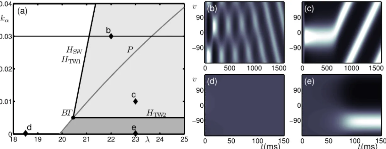
Figure 2 shows the different types of dynamical behaviour produced in different regions of the (λ, kα)-parameter plane as demarcated by bifurcation curves. The model simulations shown in

panels (b)–(e) were performed at the corresponding points in panel (a). In each case the simula-tion time was chosen such that the model reaches its stable behaviour during the simulasimula-tion; the stable behaviour is either a steady state or an oscillatory state. In the white region the model produces an homogeneous (untuned) steady-state response at a low level of activity as shown in panel (d). In the dark-grey region the model produces a steady-state response tuned to an arbi-trary direction as shown in panel (e). The boundary between the white and dark-grey regions is a pitchfork curve P ; as λ is increased and the pitchfork bifurcation is encountered the homogeneous steady-state becomes unstable and a ring of tuning curves forms the stable behaviour. In the light-grey region the stable behaviour is a travelling-wave solution with an arbitrary direction in v; the transient behaviour observed before reaching this stable state changes dependent on the chosen parameter values; see panels (b) and (c). The boundary between the white region and the

light-grey region is the coinciding Hopf-type curves HSWan HTW1. As λ is increased and the two

coinciding bifurcation points are encountered the homogeneous steady states loses stability and two new branches bifurcate simultaneously: an unstable branch of standing wave solutions and a stable branch of travelling wave solutions; this will be shown explicitly in Sec. 3.3. In panel (b), close to these curves, the unstable standing wave solution is seen as a transient behaviour before eventual convergence to the stable travelling wave solution. The boundary between the dark-grey and light-grey region is HTW2and as kαis increased and the bifurcation is encountered the stable

tuned response becomes spatially unstable and starts to travel in an arbtirary direction. In panel (c) the unstable tuned response is seen as a transient behaviour before starting to travel. . . 18 19 20 21 22 23 24 25 0 0.01 0.02 0.03 0.04 0 500 1000 1500 −90 0 90 0 500 1000 1500 −90 0 90 0 50 100 150 −90 0 90 0 50 100 150 −90 0 90 (a) (b) (c) (d) (e) HSW HTW1 HTW2 BT P b c d e λ k_α t(ms) t(ms) v v

Figure 2: Bifurcation diagram for the no-input case; summary of results from Curtu and Ermen-trout (2004) in terms of stable behaviour. (a) Bifurcation curves plotted in the (λ, kα)-parameter

plane demarcate regions with qualitatively different dynamics. The Hopf-type curves are HSW,

HTW1 (coinciding) and HTW2, a pitchfork curve is P and these curves meet at the

Bogdanov-Takens point BT . Panels (b)–(e) show the activity p(v, t) indicated by intensity for model simulations at parameter values from the corresponding points b–e in panel (a).

3.2

Simple input with k

= 0.001

Figure 3 shows a new bifurcation diagram after the introduction of the simple input I1D shown

in Fig. 1(c) with input gain kI = 0.001. We are interested to see how the solutions identified in

the previous section change and how their organisation in parameter space has been modified. The most notable result is that much of the structure from the no-input case has been preserved, albeit with subtle changes that are now discussed. In the white region (to the left of HSW1and bP)

there is now a low-activity response that is weakly tuned to the input centered at v = 0; see panel (d). In the dark-grey region there is still a steady-state, tuned response, but now centered on the stimulus at v = 0. In the light-grey region the stable behaviour is still predominantly a travelling wave solution resembling those shown in Fig. 2(b) and (c) but with a slight modulation as the wave passes over the stimulus; the modulated solution will be shown later. Here we highlight a qualitatively different type of travelling wave solution that can be found close to the Hopf curve HTW2, whereby the wave has been pinned to the stimulated direction, as a so-called slosher state

(Folias, 2011; Ermentrout et al, 2012); see panel (c). Furthermore, a new elongated region in parameter space has opened between HSW1 and the coinciding curves HSW2 and HTW1, in which

. . 18 19 20 21 22 23 24 25 0 0.01 0.02 0.03 0.04 0 500 1000 1500 −90 0 90 0 1000 2000 −90 0 90 0 50 100 150 −90 0 90 0 50 100 150 −90 0 90 (a) (b) (c) (d) (e) HSW1 H TW1 HSW2 HTW2 b P F ⇠ ⇠ ⇠ 9 b c d e DH -λ kα t(ms) t(ms) v v

Figure 3: Bifurcation diagram for the simple input case with kI = 0.001. (a) Bifurcation curves

plotted in the (λ, kα)-parameter plane demarcate regions with qualitatively different dynamics.

The Hopf curves are HSW1, HTW2, along with the coinciding HSW2and HTW1; a further Hopf in

the light-grey region involves only unstable solutions and is not labelled; all the Hopf curves meet at a the double Hopf point DH. Two bifurcation curves resulting from the symmetry breaking of a pitchfork bifurcation are bP and F ; see Fig. 4 and accompanying text. Panels (b)–(e) show the activity p(v, t) indicated by intensity for model simulations at parameter values from the corresponding points b–e in panel (a).

In order to describe in detail the changes to bifurcation structure that occur when the stimulus is introduced we now consider several one-parameter slices in λ at fixed values of kα taken from

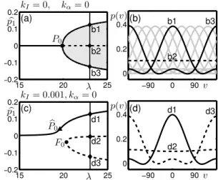
the diagrams already shown in Figs. 2(a) and 3(a); these slices are indicated by horizontal lines. Figure 4 shows one-parameter bifurcation diagrams with zero adaptation gain kα = 0, first

with no input in panel (a) and with a small simple input (kI = 0.001) in panel (c). In order to

best represent the solution branches we plot them in terms of the even, first-order mode of the solutions bp1 (the cos(v)-component). Figure 4(a) shows that for small λ there is a single, stable

solution branch with bp1= 0; this corresponds to the flat (untuned) response shown in Fig. 2(d).

When λ is increased beyond the pitchfork P0, this flat state loses its stability and a ring of

tuned responses are created. Figure 4(b) shows the profiles of the different solutions that exist at λ = 23. The dashed curve b2 is the unstable flat state, the tuned state b1 centered at v = 0 corresponds to when bp1 is largest and the tuned state b3 centered at v = ±180 corresponds to

when bp1 is smallest. Due to the presence of translational symmetry, intermediate states centered

at any value of v also exist; discrete examples of these are shown as grey curves, but note these exist on a continuous ring filling in the direction space v. The easiest way to see the effect of introducing the stimulus and the fact that this breaks the translational symmetry is by studying the states that exist in the small input case also at λ = 23 shown in Fig. 4(d). Now the only stable solution is the tuned response d1 centered at v = 0, there is a counterpart unstable solution centered at v = ±180 and all of the intermediate states have been destroyed. In the bifurcation diagram Fig. 4(c) the pitchfork bifurcation has been destroyed and there remain two disconnected solution branches. On the unstable branch the unstable solutions d2 and d3 are connected at a fold point F0; this bifurcation is traced out as F in Fig. 3(a). On the (upper)

stable branch there is a smooth transition with increasing λ from a weakly- to a highly-tuned response centered at the stimulated direction. It is useful to detect where the increase in bp1 is

. . 15 20 25 −0.2 −0.1 0 0.1 0.2 15 20 25 −0.2 −0.1 0 0.1 0.2 −90 0 90 0 0.2 0.4 −90 0 90 0 0.2 0.4 kI= 0, kα= 0 kI= 0.001, kα= 0 (a) (c) (b) (d) P0 b P0 F0 b1 b2 b3 b1 b2 b3 d1 d2 d3 d1 d2 d3 λ λ v v b p1 b p1 p(v) p(v)

Figure 4: Symmetry breaking of the pitchfork with introduction of a stimulus. (a) and (c) show bifurcation diagrams in λ for the no-input and small input cases, respectively; stable states are solid curves and unstable states are dashed curves. (b) and (d) show the solution profiles in v-space at the labelled points for λ = 23; stable states are solid curves and unstable states are dashed curves. In panel (b) the solid black curves correspond to the solution b1, for which b

p1 takes its largest value and the solution b3, for which bp1 takes its smallest value; several

intermediate solutions are plotted as grey curves, see text.

steepest as this signifies the transition to a tuned response. We denote this point bP0 and as this

is not strictly a bifurcation point we call it a pseudo pitchfork; it is still possible to trace out where this transition occurs in the (λ, kα)-plane and this is plotted as bP in Fig. 3(a).

3.3

Explanatory one-parameter bifurcation diagrams

Figure 5 shows one-parameter bifurcation diagrams in λ for three different cases:

• No input cases with kα= 0.03; see Fig. 5(a)–(c); corresponds to the horizontal line through

the point labelled b in Fig. 2(a).

• First small, simple input case with kα = 0.03; see Fig. 5(d)–(f); corresponds to the

hori-zontal line through the point labelled b in Fig. 3(a).

• Second small, simple input case with kα = 0.01; see Fig. 5(h)–(j); corresponds to the

horizontal line through the point labelled c slice in Fig. 3(a).

In order to best represent the solution branches we plot them in terms of the maximum of the sum of the even and odd first-order mode of the solutions max{ bp1+ bp2} (the cos(v) and

sin(v)-components). Figure 5(a) shows that two solution branches bifurcate simultaneously off the trivial branch at the twice-labelled point Htw1Hsw. In panel (b) we show one period of a

stable travelling wave solution from the branch corresponding to Htw1; the wave can take either

positive or negative (shown) direction in v. In panel (c) we show one period of an unstable standing wave solution from the branch corresponding to Hsw1; the standing wave oscillates such

that 180◦_{-out-of-phase (in v) maxima form alternatively. The phase in v of the entire waveform}

is arbtirary and, as for the pitchfork bifurcation, any translation of the whole waveform in v is also a solution. With the introduction of a stimulus, as for the pitchfrok bifurcation discussed

. . 20 21 22 0 0.05 0.1 0.15 20 21 22 0 0.05 0.1 0.15 18 20 22 24 0 0.1 0.2 0 T −90 0 90 0 T −90 0 90 0 T −90 0 90 0 T −90 0 90 0 T −90 0 90 0 T −90 0 90 b p1+ bp2 b p1+ bp2 b p1+ bp2 λ λ λ kI= 0, kα= 0.03 kI= 0.001, kα= 0.03 kI= 0.001, kα= 0.01 (a) (b) (c) (d) (e) (f) (h) (i) (j) b c e f i j Htw1Hsw Hsw1 XXz Hsw2 ⇠ ⇠ 9 Htw1 PS b P0 _Htw2 v v v v v v

Figure 5: Changes to standing- and travelling-wave branches born in Hopf bifurcations with introduction of the stimulus. The first column shows one-parameter bifurcation diagrams in λ where black curves are steady-state branches and grey periodic branches; stable solution branches are solid and unstable branches are dashed. Hopf bifurcations to travelling waves are Htw1 and

Htw2, and to standing waves are Hsw, Hsw1, and Hsw2. Second and third columns show one period

T of the solutions at corresponding points on solution branches from one-parameter diagrams.

earlier, the translational symmetry of the solutions is broken resulting in changes to the solution structure. The bifurcation point Hswshown in Fig. 5(a) splits into two bifurcation points Hsw1

and Hsw2 in panel (d) and solution profiles on the respective bifurcating branches are shown in

panels (e) and (f). On the first branch, which is initially stable close to Hsw1, one of the maxima

is centered on the stimulated direction v = 0◦_{. For the second unstable branch bifurcating from}

Hsw2 the maxima are out of phase with the stimulated direction. The travelling wave branch is

now a secondary bifurcation from the branch originating at Hsw1 and the solutions now have a

small modulation when the travelling wave passes over v = 0◦ _{(similar to the solution shown}

in panel (j)). In panel (h), at a lower value of kα, the steady-state solution branch is initially

weakly tuned and forms a highly-tuned solution after bP0. The tuned response becomes unstable

at Htw2; close to this bifurcation point the solution is pinned by the stimulated direction, as was

shown in Fig. 3(c), and as λ is increased further the amplitude in v of these oscillations about the stimulated direction increases, see panel Fig. 5(i). When the point PS is reached in panel (h) the oscillations become large enough such that there is a phase slip and beyond this point we obtain a standard travelling wave solution once more, see panel (j). Note that the travelling wave is still modulated as it passes over the stimulated direction. We reiterate the qualitative difference between the branches forming at Htw1 and Htw2: for branches of travelling wave forming directly

from an untuned or weakly tuned steady state as at Htw1 the solutions cannot be pinned to

steady state as at Htw2the solutions are pinned to a stimulated direction close to the bifurcation.

Furthermore, we note that, with the introduction of a stimulus a region of stable standing wave solutions, in phase with the stimulated direction, are introduced between Hsw1 and Htw1; see

branch segment through the point e in Fig. 5(d).

The bifurcation analysis with the same input studied throughout this section, as shown in Fig. 1(c), continues in the next section. We go on to present the case kI = 0.01 but in the context

of a motion stimulus.

4

Competition model applied to the study of multistable

motion

We now extend the general study presented in Sec. 3 and demonstrate how the same model can be used to study a specific neural biological phenomenon for which perceptual shifts are observed. We now associate the model’s periodic feature space v 2 [−π, π) with motion direc-tion. We assume that the model’s activity in terms of time-evolving of firing rates p(v, t) are responses of direction-selective neurons in the middle temporal (MT) visual area. Indeed, MT is characterised by direction-selective neurons that are organised in a columnar fashion (Diogo et al, 2003). Here we only consider a feature space of motion direction and, thus, we assume the model responses to be averaged across physical (cortical) space. The chosen connectivity func-tion Eq. (4) shown in Fig. 1(b) represents mutual inhibifunc-tion between sub-populafunc-tions of neurons associated with competing directions; this type of connectivity naturally gives rise to winner-takes-all responses tuned to one specific direction; there is evidence that competing percepts have mutually inhibitory representations in MT (Logothetis et al, 1989; Leopold and Logothetis, 1996)). We use the models tuned response to dynamically simulate the mechanisms driving per-ception; cortical responses of MT have been linked specifically to perception of motion (Britten, 2003; Serences and Boynton, 2007). We assume that over time any particular tuned response will slowly be inhibited as represented by the linear spike-frequency adaptation mechanism in the model. Furthermore, we assume there to be a fixed-amplitude stochastic fluctuation in the membrane potential that is modelled by additive noise (note that the noise is only introduced for the simulations presented in Sec. 5). We use as a model input pre-processed direction sig-nals in the form expected from V1 (Britten, 2003; Born and Bradley, 2005). In Sec. 4.2 the model’s response properties in terms of its contrast dependence and direction tuning properties will be matched to what is known about the direction selective behaviour of MT neurons from physiological studies (Albright, 1984; Sclar et al, 1990; Diogo et al, 2003).

4.1

Definition of motion stimuli

We introduce two classical psychophysical stimuli where a luminance grating drifting diagonally (up and to the right in the example shown) is viewed through an aperture see Figs. 6(a) and (b). In the first case, with a circular aperture, the grating is consistently perceived as moving in the diagonal direction D (v = 0◦_{). The classical barberpole illusion (Hildreth, 1983, Chapter 4)}

comes about as a result of the aperture problem (Wallach, 1935; Wuerger et al, 1996), a diagonally drifting grating viewed through an elongated rectangular aperture is perceived as drifting in the direction of the long edge of the aperture. In the second case, with a square aperture, the stimulus has been shown to be multistable for short presentations on the order of 2–3s, where the dominant percepts are vertical V (v = 45◦_{), horizontal H (v = −45}◦_{) and D (v = 0}◦_{) (Castet}

et al, 1999; Fisher and Zanker, 2001). We denote this stimulus the multistable barberpole and it has been the subject of complementary psychophysical experiments (Meso et al, 2012b) from

which some results will be presented in Sec. 5.2. . . −90 0 90 0 0.5 1 −90 0 90 0 0.5 1 −90 0 90 0 0.5 1

Simple visual stimulus:

Complex visual stimulus:

1D motion signals:

2D motion signals:

Complex model input: D(v = 0 ◦) D(v = 0◦) H (v = −45◦₎ V( v =4 5 ◦) ? 6 w1D (a) (b) (c) (d) (e) v v v I1D(v) I2D(v) Iext(v)

Figure 6: Simple and complex motion stimuli. (a): A drifting luminance grating viewed through a circular soft aperture; the diagonal direction of motion D is consistently perceived. (b): A drifting luminance grating viewed through a square aperture; the dominant percepts are vertical V, horizontal H and diagonal D. (c): Representation of the 1D motion signals in direction space; the simple motion stimulus (a) is equated with I1D. (d): Representation of the 2D motion signals

in direction space. (e): Summation of the 1D and 2D motion signals with a weighting w1D= 0.5;

the complex motion stimulus (b) is equated with Iext.

It has been shown in Barthélemy et al (2008) the motion signals from 1D cues stimulate a broad range of directions when compared with 2D cues that stimulate a more localised range of directions; see arrows in Figs. 6(a) and (b). Based on these properties, it is proposed that the multistability for the square-aperture stimulus is primarily generated by competition between ambiguous 1D motion direction signals along grating contours on the interior of the aperture and more directionally specific 2D signals at the terminators along the aperture edges. We represent the 1D cues by a Gaussian bump I1D(v) = exp(−v2/2σ1D2 ) with σ1D= 18◦ centred at v = 0◦ as

shown in Fig. 6(c) (which is the same as Fig. 1(c)); on its own we call this a simple input that represents a drifting grating either filling the visual field (without aperture) or with an aperture that has no net effect on perceived direction such as the circular one shown in Fig. 6(a). We represent the 2D cues by two Gaussian bumps I2D(v) = exp(−v2/2σ2D2 ) centred at v = 45◦and

v = −45◦ _{with width σ}

2D = 6◦ as shown in Fig. 6(d). Note that the functions I1D and I2D are

normalised such that their maxima are 1 (not their areas). Figure 6(e) shows the complex input Iext represented as a summation of 1D and 2D motion signals with maximum normalised to 1

and a smaller weighting w1D2 [0, 1] given to 1D cues:

Iext(v) = w1DI1D(v) + I2D(v − 45) + I2D(v + 45). (7)

The weighting w1D translates the fact that in motion integration experiments 2D cues play a

Barthélemy et al, 2010). Here we represent this weighting in a simple linear relationship, but in future studies it may be relevant to consider the contrast response functions for 1D and 2D cues separately (Barthélemy et al, 2008).

4.2

Simple input case with k

= 0.01

: parameter tuning for motion

study and contrast dependence

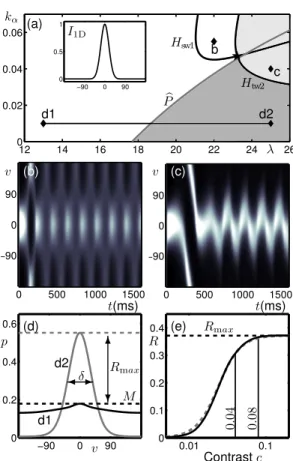
Figure 7(a) shows the two-parameter bifurcation diagram in λ and kα for the same simple 1D

input as in Fig. 3(a), but with input gain increased by a factor of 10 to kI = 0.01. The

diagram shows the same organisation of bifurcation curves, but the oscillatory regions have shifted significantly towards the top-right corner. Once again, in the white region containing the point d1 there is a steady, low-activity, weakly tuned response; see lower curve in panel (d). In the dark grey region containing the point d2 there is a steady, high-activity, tuned response with tuning width δ; see upper curve in panel (d). We define δ as the width at half-height of the tuned response. Again, the boundary between these regions is demarcated by bP in Fig. 3(a). In the region containing the point b there is still a standing-wave-type solution, but it has been modified by the input such that there are oscillations between a tuned and an untuned state over time; see Fig. 7(b). In this context there is not a physiological interpretation for this solution, and so we will ensure that the model is operated in a parameter region where it cannot be observed. In the region containing the point c there is still a periodic response with small-amplitude oscillations in v of a tuned response about v = 0; see Fig. 7(c). This is a travelling-wave-type slosher solution as described in Sec. 3.2 that is pinned by the input at v = 0◦_{; note the transient that makes one}

full excursion before being pinned. Closer to the bifurcation curve the solutions are immediately pinned and further away a phase slip can be encountered as shown in Fig. 5(h)–(j). For a simple (unambiguous) input we again operate the model away from this oscillatory region of parameter space but find that when the complex input is introduced it is the slosher-type solutions that produce the desired switching behaviour.

In order to produce results and predictions that can be related directly to the experiments, where contrast was one of the main parameter investigated, contrast should also be represented as a parameter in the model. We argue that motion signals arriving in MT, primarily from V1, are normalised by shifts in the sigmoidal nonlinearity (Carandini and Heeger, 2011) and, therefore we should not vary the input gain kI in Eq. (1) with respect to contrast. Accordingly, we found that

when the input gain kI is increased, the model ceased to produce switching behaviour. However,

by making the slope parameter λ depend on the contrast c 2 [0, 1], we are able to reproduce the observed switching behaviour.

We now fix kα = 0.01 such that we operating the model away from the oscillatory regions

shown in Fig. 7 and describe how the model can be reparametrised in terms of contrast c. For some steady state ¯p, we define firing rate response R = max{¯p} − M as the peak firing rate response above some baseline value M; max{¯p} is shown as a dashed line for solutions d1 and d2 in Fig. 7(d) and we set M = max{¯pd1}. As discussed in more detail in the Appendix B, the

solution d1 at λ = 13 is consistent with an MT response to a very low contrast input (c < 0.01), whereas the solutions d2 at λ = 25 is consistent with a high contrast input (c > 0.2). By making λ a specific function of c we are able to match the model’s contrast response to known behaviour for MT neurons. As shown in Fig. 7(e), we match the model’s response to an appropriately parametrised Naka-Rushton function, which was used to fit contrast response data across several stages of the visual pathway including MT in Sclar et al (1990); again, refer to Appendix B for further details. The operating range for the model is indicated by a horizontal line at kα= 0.01

for λ 2 [13, 25] in Fig. 7(a). In Appendix B we also show that the tuning widths δ of the model responses are in agreement with the literature (Albright, 1984; Diogo et al, 2003).

. . 0 500 1000 1500 −90 0 90 0 500 1000 1500 −90 0 90 12 14 16 18 20 22 24 26 0 0.02 0.04 0.06 −90 0 90 0 0.5 1 Hsw1 Htw2 b P (a) (b) (c) I1D d1 d2 b c kα λ v v 0.01 0.1 0 0.1 0.2 0.3 0.4 −90 0 90 0 0.2 0.4 0.6 t(ms) t(ms) p ₆ ? Rmax M (d) d1 d2 -$δ v Rmax (e) Contrastc R 0. 04 0. 08

Figure 7: Bifurcation study and contrast response for simple input I1D (see inset of (a)) with

input gain kI = 0.01. (a): Two-parameter bifurcation diagram in terms of sigmoid slope λ

and adaptation strength kα shows qualitatively the same organisation of bifurcation curves as

Fig. 3(a). (b),(c): Time-traces of the activity p(v, t) indicated by intensity as computed at the corresponding points b and c labelled in (a). (d): Steady-state responses in terms of the activity p(v) at the corresponding points d1 and d2 labelled in (a). (e): Contrast response in terms of normalised peak activity R for simple input (solid curve) fitted to a Naka-Rushton function (dashed curve) as described in Appendix B. The line between d1 and d2 in (a) is the operating range of the model. The response d1 shown in panel (d) corresponds to c = 0 and the response d2 in panel (d) corresponds to c = 1.

4.3

Complex input with k

= 0.01

In the following sections an adaptation timescale of τα = 16.5s is used, which is consistent

with reported values from physiological experiments (Descalzo et al, 2005). Up until now the results presented have been carried out with the adaptation timescale arbitrarily fixed at τα=

100ms. The change of timescale does not qualitatively change the bifurcation diagrams shown previously or in the present section. However, it does change the oscillations produced such that they reproduce the type of switching observed in the experiments that will be discussed in Sec. 5.2; indeed, the specific value of ταwas chosen to match experimental data. In order for the

bifurcation results described in earlier sections to be relevant it is desirable that we work with a small-amplitude additive noise as governed by kX. The single source of noise in the model

evolves with its timescale τX set equal to τα. This choice was found to have a pronounced affect

on the switching dynamics without the need for large values of kX. Note that the time units

displayed in figures up to this point are ms, but will be s in the remainder of the paper. Figure 8 shows the bifurcation diagram for a complex input and the different types of be-haviour that are observed in the operating range of the model as defined in the previous section. In the presence of the complex input, we see the same four regions found for the simple input; compare Fig. 7(a) and Fig. 8(a). The top-right-most region of the (λ, kα)-plane in which

oscil-lations about v = 0◦ _{are observed has grown significantly. As for the simple input, there is a}

weakly tuned steady-state response in the region containing the point b and there is a tuned steady-state response in the region containing the point c; see panels (b) and (c). However, the region contaning the point d now shows an altered oscillatory behaviour. We see a model re-sponse that is initially centred at the direction D but after 2–3s shifts to H and proceeds to make regular switches between H and V, see panel (d). The model’s separation of timescales is now seen more clearly; the model spends prolonged periods at H or V during which the adaptation builds up and eventually induces a switch to the opposite state; with τα= 16.5s switches occur

every ⇡ 3s, but the transition itself takes only ⇡ 50ms. Due to the dynamics being deterministic in the absence of noise (kX = 0), the switches occur at regular intervals.

As described in the previous section we fix the operating region of the model with kα= 0.01

and for λ 2 [13, 25] as indicated by the horizontal line in Fig. 8(a). As λ is increased from λ = 13 at b to λ = 25 at d (equivalently contrast increases from c = 0 to c > 0.2) there are transitions from a weakly tuned response (b) to a tuned response (c) to an oscillatory response (d). For c > 0.2 the model response saturates as shown in Fig. 7(e). We now incorporate another known aspect of contrast dependence in motion processing by varying the relative weighting between 1D and 2D cues in the input. The psychophysics experiments presented in Lorenceau and Shiffrar (1992); Lorenceau et al (1993) show that 1D cues (contour signals) play an important role in motion perception at low contrast that diminishes with increasing contrast. As contrast increases the 2D cues (terminator signals) play a more significant role. Based on these studies we propose that for the complex model input (7) the relative weighting of 1D cues should decrease linearly with contrast

w1D= W0− W1c, (8)

where W0 = 0.5 and W1 = 1.1. These specific values were chosen in order to match the

experi-ments; see further comments in Sec. 5.3.

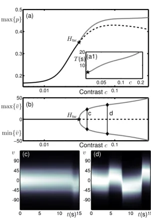
Figure 9 shows a one-parameter bifurcation diagram for the model working in the operating regime shown in Figs. 7(a) and 8(a) but now reparameterised in terms of contrast c as described above. At low contrast there is a stable steady-state response tuned to the direction D. The peak response max{p} increases with contrast. This steady-state response loses stability at a travelling-wave Hopf instability Htwbeyond which there is a stable oscillatory branch. The

. . !" !# !$ !% "& "" "# "$ & &'&" &'&# &'&$ −90 0 90 0 0.5 1 0 5 10 15 −90 0 90 0 5 10 15 −90 0 90 0 5 10 15 −90 0 90 Hsw1 Htw2 b P (a) Iext kα λ b c d t(s) t(s) t(s) (b) (c) (d) v v v H D V

Figure 8: Bifurcation study for complex input Iext (see inset of (a)) with input gain kI = 0.01.

(a): Two-parameter bifurcation diagram in terms of sigmoid slope λ and adaptation strength kα shows qualitatively the same organisation of bifurcation curves as Fig. 3(a) and Fig. 7(a).

Line between points labelled b and d in (a) show the operating region of the model as defined in Fig. 7(a). (b)–(d): Time-traces of the activity p(v, t) indicated by intensity as computed at the corresponding points b, c and d labelled in (a).

. . 0.01 0.1 0.2 0.3 0.4 0.5 0.05 0.1 0.2 10 20 0.01 0.1 −50 0 50 (a) (b) c (a1) T (s) Contrastc Contrastc max{p} max{¯v} min{¯v} Htw Htw c d v v t(s) t(s) (c) (d)

Figure 9: Bifurcation diagram with complex input for model parameterised in terms of contrast. (a),(b): One-parameter bifurcation diagrams show the same data plotted in terms of the maxi-mum response and average direction, respectively; the steady-state response tuned to D is solid black when stable and dashed black when unstable. Stable branch of oscillations between H and V is grey. (a1): The period on the oscillatory branch. (c),(d): Time-traces of the activity p(v, t) indicated by intensity as computed at the corresponding points c and d labelled in (b).

unstable branch associated with the D direction decreases in max{p} at large contrasts; see dashed curve in panel (a). Secondly, the period and amplitude of the oscillations in ¯v does not saturate but continues to increase with contrast as shown in the inset (a1) and panel (b). We also note that close to the bifurcation point Htwthere are long transients before the onset of

oscillations, see panel (c), and that further from the bifurcation point the onset of oscillations is faster, see panel (d).

5

Comparison of model with experimental results

5.1

Experimental results

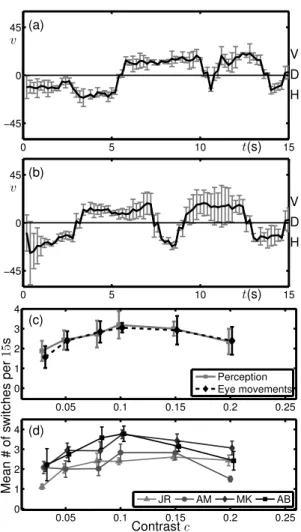
Figure 10 shows a summary of experimental data obtained in psychophysics experiments using the complex stimulus shown in Fig. 6(b) Meso et al (2012b). Data was recorded from four subjects for 15s presentations of the stimulus. Eye movements were recorded and continuous smooth trajectories estimated after removing blinks, saccades (very fast abrupt movements) and applying a temporal low pass filter. An SR Eyelink 1000 video recorder was used for the eye movement recordings and psychophysics stimuli were presented on a CRT monitor through a Mac computer using Psychtoolbox version 3.0 running stimulus generation routines written in Matlab. For the specific data shown, four healthy volunteers who provided their informed consent were participants, of whom two were naive to the hypothesis being tested. All experiments were carried out with, and following CNRS ethical approval. The presented stimuli covered 10 degrees of visual angle (the size of the side of the square in Fig. 6(b)) and were presented at a distance of 57cm from the monitor. Each task was done over 8 blocks of up 15 minutes over which 36 trials spanning a range of six contrasts were randomly presented each time. In this paradigm, recorded forced choice decisions indicating shifts in perceived direction through the three directions H, D and V and the estimated eye directions were found to be coupled and both indicative of perceived direction. Further details of these experiments can be found in our previous presentation (Meso et al 2012b) and a full description will appear in the experimental counterpart of this manuscript. The temporal resolution of the eye traces is much higher than that of the reported transi-tions and allows for a relatively continuous representation of eye movement direction that can be compared with model simulations. Figure 10(a) and (b) show, for two different subjects, time traces of the time-integrated directional average of eye-movements from a single experimental trial at c = 0.08. Switches in perception can be computed from these trajectories by imposing thresholds for the different percepts. Both trials show that the directions H and V are held for extended durations and regular switches occur between these two states. The switches involve sharp transitions through the diagonal direction D. The diagonal direction can be held for ex-tended durations immediately after presentation onset. However, we note that the eye-movement direction during the first 1s of presentation has a more limited history in its temporal filtering. Short presentations of the same stimulus were investigated in a related set of experiments (Meso et al, 2012a) and modelling work (Rankin et al, 2012).

Figure 10 also shows the relationship between the averaged rate of switches between H and V over a range of contrast values c 2 {0.03, 0.05, 0.08, 0.1, 0.15, 0.2}; in panel (c) the data is averaged across the four subjects and in panel (d) it is separated out by subject. The lowest contrast shown c = 0.03 corresponds to the smallest contrast value for which subjects were able to reliably report a direction of motion for the stimulus. For the grouped data, at low contrast (c < 0.1) the rate of switching increases with contrast with the rate being maximal at approximately c ⇡ 0.1. Beyond the peak, for contrasts c > 0.1, the rate of switching decreases with contrast. For the data separated by subject shown in panel (d), the subjects MK and AB have a peak rate around 3.5 switches per 15s presentation and the peak occurs at c ⇡ 0.1. For

subjects JR and AM the peak rate is lower at around 2.5 switches per 15s presentation and there is a less prominent peak occurring at a higher contrast value c > 0.1. However, the common pattern reveals two qualitatively different regimes with respect to changing contrast. A low contrast regime for which the switching rate increases with contrast and a high contrast regime for which the switching rate decreases with contrast.

5.2

Model simulations with noise (k

= 0.0025

)

We now study the dynamics of the model in the presence of additive noise in the main neural field equation. Recall that the stochastic process in the model is operating on the same slow timescale τα as the adaptation and that the strength of the noise is kX = 0.0025. Two cases

will be studied, first the low contrast case at c = 0.04, close to the contrast threshold on the steep part of the model’s contrast response; see Fig. 7(e). Second, the high contrast case at c = 0.08, which is above the contrast threshold on the saturated part of the contrast response function. In the first case, noise is introduced in a parameter regime where the model is close to bifurcation and oscillations only occur after a long transient, see Fig. 9(c). When operating in a nearby parameter regime close to bifurcation the noise causes random deviations away from the direction D and can drive the model into an oscillatory state more quickly. In the second case, noise is introduced in a parameter regime where the model produces an oscillatory response with a short transient behaviour, see Fig. 9(d). In this regime the noise perturbs the regular oscillations either shortening or prolonging the time spent close to H and V.

Figure 11(a)–(d) shows 15s time traces of the population activity p for the cases c = 0.04 (first row) and c = 0.08 (second row). Note that each individual model simulation is quite different due to the noise, but we have selected representative examples that allow us to highlight key features in the model responses and compare the different contrast cases. In processing this simulated data we assume that, initially the activity is centred around the direction D, and after some transient period switching will occur primarily between H and V. In order to detect switches between the directions H and V a so-called perceptual threshold (P T ) has been set at v = ±10◦_.

The first switch from D to either H or V is detected the first time the corresponding threshold is crossed. Subsequent switches are only detected the next time the opposite threshold is crossed. Note that although other algorithms could be employed to detect these switches, we found that these do not have had a great effect on the presented results.

Across all the examples shown in Fig. 11, the average direction ¯v oscillates in a random fashion and as time progresses the amplitude of these oscillations grows in v. For the case c = 0.04 there is a long transient and the first switch occurs for approximately t 2 [5s, 10s]. For the case c = 0.08 the overall amplitude of the oscillations is larger and the first switch occurs for t < 3s. Note also that the level of activity shown as an intensity in Fig. 11 is higher in the c = 0.08 case. An important difference between the two contrast cases is that in the low contrast case, the transitions between H and V occur gradually when compared with the abrupt transitions in the high contrast case. This suggests that at low contrast the direction D could be seen during the transitions, where as in the high contrast case the switches occur directly from H to V.

With respect to the experimental data, the model consistently reproduces the characteristic behaviour of regular switches between the H and V. Furthermore, the sharp transitions through the diagonal direction D are also captured well by the model. Compare the second row of Fig. 11 with the two examples shown in Fig. 10(a) and (b).

. . 0 5 10 15 −45 0 45 0 5 10 15 −45 0 45 0.05 0.1 0.15 0.2 0.25 0 1 2 3 4 Perception Eye movements 0.05 0.1 0.15 0.2 0.25 0 1 2 3 4 JR AM MK AB H D V H D V t(s) t(s) v v Contrastc Mean # of switches per 15 s (a) (b) (c) (d)

Figure 10: Summary of results from psychophysics experiments for the complex stimulus shown in Fig. 6(b). (a), (b): Time traces of average direction from eye-movements during two individual stimulus presentations at c = 0.08. Error bars show the standard deviation of the computed direction of smooth components over 200 samples; the re-sampled value at 5Hz is the mean. (c): Relation between contrast and mean switching rate in terms of perception (reported by subjects) and as computed from eye-movement traces; grouped data is averaged across the four subjects with standard error shown. (d): Switching-rate data (from perception) separated out by subject with standard error for each subject shown.

. . Modelc = 0.08 Modelc = 0.04 t(s) t(s) t(s) t(s) (a) (c) (b) (d) H D V H D V H D V H D V v v v v

Figure 11: Time traces from individual model simulations where intensity shows the population activity across direction space (vertical axis). The solid black line is the average of this activity (average direction ¯v) and the dashed lines indicate perception thresholds (P T ) for detection of switches between the directions H and V; switches are indicated by vertical white lines. First and second rows shows examples from the low and high contrast cases, respectively.

5.3

Dependence of switching rate on contrast

Figure 12 shows the relationship between contrast and switching rate as computed with the model where the rate is expressed as the mean number of switches per 15s simulation. Panel (a) shows the relationship without noise (kX = 0) and with noise (kX = 0.0025). We show the

average switching rate at discrete contrasts c 2 [0.02, 0.25] and at each contrast value we plot the switching rate averaged across 500 model simulations.

The deterministic case can be explained in terms of the bifurcation diagram shown in Fig. 9. At low contrast, no switching behaviour is observed as the model can only produce a steady-state response weakly tuned to the direction D. With increasing contrast, the onset of switching is abrupt, occurring just above c = 0.04 after the bifurcation Htwat c ⇡ 0.03. Switching does not

begin immediately at the bifurcation point, due to long transients for values of c nearby, see Fig. 9(c). The switching rate remains constant at around 3 switches per 15s interval, and starts to drop off for contrasts c > 0.12. The reduction in switching rate for larger contrasts is due to the increasing period of the oscillations as shown in Fig. 9(a1).

With the introduction of noise, there is an overall increase in switching rate, however, for larger contrasts the increase is minimal. At low contrasts, when the model is operating close to bifurcation, the noise has a more pronounced effect on the dynamics. As the contrast increases from c = 0.02 there is a smooth increase in the rate of switching, which peaks after the bifurcation point before starting to decrease as in the no-noise case. Mechanistically these results can be interpreted as follows: at larger contrasts the switching rate is governed by an underlying adaptation driven oscillation. When noise is introduced, the individual switching times are randomly distributed as will be discussed in Sec. 5.4, but the average rate is not affected as can be seen by comparing the two cases shown in Fig. 12(a). At lower contrasts the presence of noise alone can drive a deviation from the diagonal direction leading to a switch. However, because the model is operating close to bifurcation the noise can also serve to shorten the transient period before the onset of adaptation-driven switching. Note that the intensity of noise is fixed across all contrasts, it is only at low contrasts that this has a large effect on the underlying dynamics. The model results with noise are able to accurately capture the two contrast regimes from the experimental data. That is to say, an increase in switching rate at low contrasts with peak and subsequent decrease in switching rate at higher contrasts, compare Fig. 12(a) black curve with Fig. 10(a). The values of W0, W1 and τα were chosen in order to fit the experimental

data, however, the two contrast regimes are robustly produced by the model independent of the specific values chosen. In Fig. 12(b) we show how, in the model, the relationship between switching rate and contrast changes with respect to P T . When P T is low the peak switching rate is highest and occurs at a low contrast value. As P T is increased, the peak rate decreases and also occurs at a higher contrast value; the relationship also appears to flatten out for larger P T . Figure 10(b) shows the reported switching rate curves from the experiments, separated out by individual subject. The data shows a range of peak switching rate between the subjects. For the two subjects with the highest switching rate (MK,AB), the prominent peak occurs at c ⇡ 0.1. For the other two subjects (JR,AM), the peak rate is lower, the response is flatter and the peak rate occurs at a larger value of c. We conclude that differences in perceptual threshold between subjects can account for inter-subject differences.

. . 0 0.05 0.1 0.15 0.2 0.25 0 1 2 3 4

No noise With noise

0 0.05 0.1 0.15 0.2 0.25 0 1 2 3 4 PT=20 17 14 11 Contrastc Mean # of switches per 15 s Htw (a) (b)

Figure 12: Mean switching rates computed with the model and recorded from psychophysics experiments. (a): Switching rates computed with the model without noise and with noise. (b): Switching rate curves computed with the model for a range of P T values.

5.4

Distribution of switching times

In the previous section we showed example model outputs for which switches between the di-rections H and V are detected. We found that the times between these switches vary and that, particularly in the low contrast case, the early transient behaviour can be very different from one simulation to the next. In order to investigate the distribution of the switching times we ran 1, 500 model simulations each of 15s and formed a data set by extracting the times between consecutive switches from each simulation.

Figure 13 shows histograms of the computed switching times tsw. In the low contrast case

approximately 1, 483 switches were recorded with mean time ¯tsw= 3.73s and SD= 2.89

(Coeffi-cient of Variance COV= 0.56) and in the high contrast case 3, 154 switches were reported with mean time ¯tsw = 4.07s and SD= 2.08 (COV= 0.51). Although the mean of tsw is smaller in

the high contrast case, more switches are detected because there is a shorter transient period before switching begins; the average time to the first switch in the low contrast case is 7.47s (SD= 2.87) compared with an average time of 3.02s (SD= 1.56) in the high contrast case. The aim now is to determine from which distribution the model data could have arisen. We follow the method presented in Shpiro et al (2009) and compare the model data with a Weibull prob-ability distribution function (pdf), a gamma pdf and a log-normal pdf each with parameters