HAL Id: hal-00328210
https://hal.archives-ouvertes.fr/hal-00328210v2
Submitted on 13 Dec 2007
HAL is a multi-disciplinary open access
archive for the deposit and dissemination of
sci-entific research documents, whether they are
pub-lished or not. The documents may come from
teaching and research institutions in France or
abroad, or from public or private research centers.
L’archive ouverte pluridisciplinaire HAL, est
destinée au dépôt et à la diffusion de documents
scientifiques de niveau recherche, publiés ou non,
émanant des établissements d’enseignement et de
recherche français ou étrangers, des laboratoires
publics ou privés.
upper-tropospheric methanol as revealed from space
G. Dufour, Sophie Szopa, D. A. Hauglustaine, C. D. Boone, C. P. Rinsland, P.
F. Bernath
To cite this version:
G. Dufour, Sophie Szopa, D. A. Hauglustaine, C. D. Boone, C. P. Rinsland, et al.. The influence of
biogenic emissions on upper-tropospheric methanol as revealed from space. Atmospheric Chemistry
and Physics, European Geosciences Union, 2007, 7 (24), pp.6129. �10.5194/acp-7-6119-2007�.
�hal-00328210v2�
© Author(s) 2007. This work is licensed under a Creative Commons License.
Chemistry
and Physics
The influence of biogenic emissions on upper-tropospheric methanol
as revealed from space
G. Dufour1,*, S. Szopa2, D. A. Hauglustaine2, C. D. Boone3, C. P. Rinsland4, and P. F. Bernath3,5
1Laboratoire de M´et´eorologie Dynamique/Institut Pierre Simon Laplace (LMD/IPSL), Palaiseau, France
2Laboratoire des Sciences du Climat et de l’Environnement (LSCE/IPSL), CNRS-CEA-UVSQ Gif-sur-Yvette, France 3Department of Chemistry, University of Waterloo, Ontario, N2L 3G1, Canada
4NASA Langley Research Center, Hampton, VA, USA
5Deparment of Chemistry, University of York, Heslington, York, YO10 5DD, UK
*now at: Laboratoire Inter-universitaire des Syst`emes Atmosph´eriques (LISA), Universit´es Paris 12 et Paris 7, CNRS, Cr´eteil,
France
Received: 15 June 2007 – Published in Atmos. Chem. Phys. Discuss.: 28 June 2007 Revised: 24 October 2007 – Accepted: 28 November 2007 – Published: 13 December 2007
Abstract. The distribution and budget of oxygenated
or-ganic compounds in the atmosphere and their impact on tropospheric chemistry are still poorly constrained. Near-global space-borne measurements of seasonally resolved up-per tropospheric profiles of methanol (CH3OH) by the ACE
Fourier transform spectrometer provide a unique opportunity to evaluate our understanding of this important oxygenated organic species. ACE-FTS observations from March 2004 to August 2005 period are presented. These observations re-veal the pervasive imprint of surface sources on upper tro-pospheric methanol: mixing ratios observed in the mid and high latitudes of the Northern Hemisphere reflect the sea-sonal cycle of the biogenic emissions whereas the methanol cycle observed in the southern tropics is highly influenced by biomass burning emissions. The comparison with dis-tributions simulated by the state-of-the-art global chemistry transport model, LMDz-INCA, suggests that: (i) the back-ground methanol (high southern latitudes) is correctly repre-sented by the model considering the measurement uncertain-ties; (ii) the current emissions from the continental biosphere are underestimated during spring and summer in the North-ern Hemisphere leading to an underestimation of modelled upper tropospheric methanol; (iii) the seasonal variation of upper tropospheric methanol is shifted to the fall in the model suggesting either an insufficient destruction of CH3OH (due
to too weak chemistry and/or deposition) in fall and winter months or an unfaithful representation of transport; (iv) the impact of tropical biomass burning emissions on upper tro-pospheric methanol is rather well reproduced by the model. This study illustrates the potential of these first global profile
Correspondence to: G. Dufour
(dufour@lisa.univ-paris12.fr)
observations of oxygenated compounds in the upper tropo-sphere to improve our understanding of their global distribu-tion, fate and budget.
1 Introduction
Methanol (CH3OH) is the second most abundant organic
molecule in the atmosphere after methane (Singh et al., 2001) and is the predominant oxygenated organic compound in the mid to upper troposphere (Heikes et al., 2002). Furthermore, primary methanol emissions constitute about 6% of the total terrestrial biogenic organic carbon emissions (Heikes et al., 2002). Oxygenated species such as methanol also influence the oxidizing capacity of the atmosphere by reacting with the hydroxyl radical, OH, to produce HO2and formaldehyde
(Tie et al., 2003). As such, methanol represents an important source of radicals in the dry upper troposphere and affects the budget of tropospheric ozone (Tie et al., 2003; Folberth et al., 2006). However, the existing measurements of methanol suf-fer from a very limited spatial and temporal coverage and, as a consequence, large uncertainties exist in our knowledge of the methanol distribution and budget in the atmosphere (Ja-cob et al., 2005).
The global distribution of methanol has been assessed using global chemical transport models (Tie et al., 2003; Von Kuhlmann et al., 2003; Jacob et al., 2005; Folberth et al., 2006). However, the few available surface sites (e.g., Heikes et al., 2002; Karl et al., 2003; Schade and Goldstein, 2006) and aircraft measurements (e.g., Singh et al., 2000; Singh et al., 2003) do not provide a sufficient constraint on the simulated methanol distribution. In particular, little is
(a)
a)
b)
(b)
b)
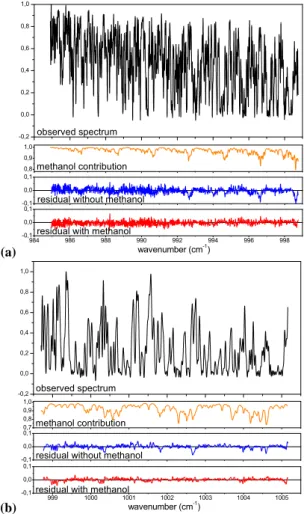
Fig. 1. (a) Spectral window used for the retrieval in Dufour et
al. (2006). (b) Additional window used for this study (see text for details). The upper panels show a spectrum observed at 10 km in the tropics during October 2004. The second panels represent the methanol contribution to the spectrum. The third and the last panels give the residuals (observed-calculated) when methanol is excluded or included in the calculation, respectively.
known about the seasonal variation of methanol, especially in the mid- to upper-troposphere. The origin of methanol in the atmosphere is largely dominated by biogenic emis-sions (Galbally and Kristine, 2002). Plant growth repre-sents up to 60–80% of this source and is responsible for a strong seasonal cycle in methanol abundance, especially in the Northern Hemisphere where vegetated land surfaces pre-vail (Jacob et al., 2005; Galbally and Kristine, 2002; Fol-berth et al., 2006). Methanol release from plants is higher for young leaves than for mature leaves (Galbally and Kris-tine, 2002; Jacob et al., 2005; Lathi`ere et al., 2006) imply-ing peak emissions in sprimply-ing and early summer (Karl et al., 2003; Schade and Goldstein, 2006). The biogenic sources of methanol from plant growth and also plant decay are subject to large uncertainties and current best estimates range from
77 to 312 Tg/year (Galbally and Kristine, 2002; Heikes et al., 2002; Tie et al., 2003; Von Kuhlmann et al., 2003; Jacob et al., 2005). Atmospheric oxidation of hydrocarbons, biomass burning, and urban activities are also identified as methanol sources and together contribute 27–55 Tg/year (Singh et al., 2001; Jacob et al., 2005). The major sink of methanol in the atmosphere is from gas-phase oxidation by the hydroxyl rad-ical OH (Heikes et al., 2002; Jacob et al., 2005). Other sinks arise from dry deposition, wet removal and oceanic uptake. As for the sources, these sinks are also not well quantified. In the Heikes et al. (2002) and Tie et al. (2003) studies, clo-sure of the budget is not achieved for example. Moreover, the role of the ocean as either a source or a sink is not com-pletely determined, although a recent study suggests that the ocean acts like a sink (Sinha et al., 2007). These loss terms result in a methanol lifetime in the atmosphere of 1–2 weeks (Galbally and Kristine, 2002; Heikes et al., 2002; Jacob et al., 2005). This lifetime implies that the methanol distribu-tion is not only affected by surface emissions and chemistry but also by atmospheric transport.
In this paper, we report on the first satellite observa-tions of the global methanol distribution in the upper tro-posphere using the Atmospheric Chemistry Experiment in-frared Fourier transform spectrometer (ACE-FTS) onboard the SCISAT satellite. The measurements are characterized in Sect. 2. The LMDz-INCA model used for the interpretation of the data is described in Sect. 3 as well as the emissions used for the simulations. The observations are discussed in Sect. 4 and compared to the model in Sect. 5.
2 ACE-FTS measurements
The ACE-FTS records solar occultation measurements with coverage between approximately 85◦S and 85◦N, and with a majority of observations over the Arctic and the Antarctic (Bernath et al., 2005). It is worth noting that the observa-tions are not equally distributed in space and time leading to an inhomogeneous global coverage (e.g., Bernath, 2006; Fu et al., 2007). The ACE-FTS has high spectral resolu-tion (0.02 cm−1) in the 750 to 4400 cm−1 range. Vertical profiles of temperature, pressure and various atmospheric constituents are retrieved from ACE-FTS spectra using a global fit approach (Boone et al., 2005). In our previous work, we were able to retrieve methanol profiles with en-hanced concentrations in biomass burning plumes (Dufour et al., 2006). We have improved our methanol retrievals by adding a supplementary 6.4 cm−1-width microwindow
cen-tred at 1001.9 cm−1 (Fig. 1). This permits us to extend the retrieval down to 6 km. The main interfering species in the spectral range used are O3and its minor isotopologues, CO2,
H2O, NH3, and C2H4. The isotopologues 1, 2 and 3 (OOO,
OO18O and O18OO, respectively) of ozone are fitted simul-taneously with methanol while the other interfering species are fixed to their retrieved values for H2O (version 2.2 of
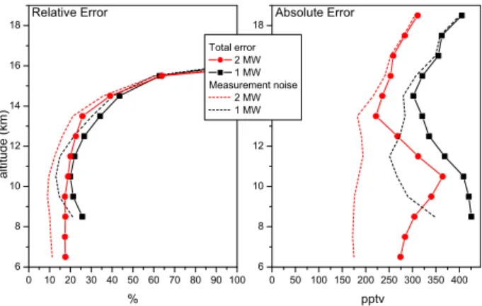
Fig. 2. Comparison of the total error and measurement noise
pro-files obtained using one or two windows for the methanol retrieval for a subset of 12 tropical retrieved profiles. The absolute error corresponds to the error expressed in concentration (pptv) and the relative error to the ratio (%) between the absolute error and the measured vmr.
the ACE-FTS operational data) or to their climatological val-ues for CO2, NH3, and C2H4. The concentration of
isotopo-logues 4 and 5 (OO17O and O17OO, respectively) of ozone is fixed using the normal isotopic abundances relative to the values of the main isotope previously retrieved.
2.1 Error determination: description of the method The statistical part of the error, corresponding to the fitting error, is named ”measurement noise”. To estimate the sys-tematic part of the error, the retrieval was performed by per-turbing each parameter by 1σ of its assumed uncertainty (Dufour et al., 2006). Error sources accounting for uncertain-ties in temperature, tangent altitude pointing, CH3OH
spec-troscopic data, instrumental line shape (ILS), and mixing ra-tios of the main interfering species (CO2, H2O, NH3, C2H4
and isotopologues 4 and 5 of ozone) are considered. The ef-fects of uncertainties in the baseline of the spectra, spectral shifts and isotopologues 1, 2 and 3 of ozone are not included in this sensitivity study because these parameters are fitted si-multaneously with methanol. Except the measurement noise, the methanol retrieval is mainly sensitive to uncertainties in the tangent height determination, in the temperature and in the spectroscopic data. The sensitivity to uncertainties in the ILS and interfering species is less than 1% on average for altitudes in the upper troposphere.
In the paper, averaged mixing ratios (vmrs) are often con-sidered. In this case, the error is reduced. However, only the statistical part of the errors decreases when vmrs are aver-aged (divided approximately by the square root of the num-ber of averaged vmrs). The resulting total error (statistical + systematic) is then driven by the systematic error and is in the 20–30% range.
Fig. 3. Methanol profiles and the associated total error profile for 5
individual occultations representative of different latitudes and sea-sons. The error profile is given only for altitudes with methanol values above the detection limit (>100 pptv).
2.2 Characterization of the retrieval errors
In order to assess the performance of our new retrieval, we compared the error budget obtained with one and two win-dows on a subset of 12 tropical occultations recorded in Oc-tober 2004 using the method described above and presented in detail by Dufour et al. (2006). The resulting measurement noise and the resulting total error obtained with one or two windows are compared in Fig. 2. Adding a new window for the retrieval improves the fitting error for concentration pro-files especially at background levels and hence permits the investigation of near global distributions for methanol. The total error at the maximum of the profile is about 17% with a two-window retrieval and about 20% with a one-window re-trieval. The errors are also more constant (in relative terms) below the tropopause with two windows and increase rapidly in the lower stratosphere.
Due to computational cost, we applied our error estima-tion method to a limited number of occultaestima-tions, selected to cover the range of measured CH3OH profiles. We then
determined the error budget for 5 individual occultations (Fig. 3). For high southern latitudes, where the methanol vmr is small (∼250 pptv), the total error reaches 80% in the troposphere and is larger than 100% in the lower stratosphere (>10 km). For other occultations, the errors usually remain below 30% in the troposphere and also increase rapidly in the lower stratosphere where the methanol concentrations de-crease rapidly. For the present study, we used a selection of profiles from March 2004 to August 2005 that sample low in the troposphere and for which the quality of the retrieval has been checked. Mean observed methanol in the upper tro-posphere for different regions of the world are reported by season in Table 1. The observations agree well with previ-ous aircraft measurements (Singh et al., 1995; Singh et al., 2000; Singh et al., 2001; Singh et al., 2004). The back-ground methanol vmr measured, for instance, from aircraft in
Africa
Europe
North-America
South-America
Asia
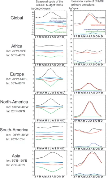
Seasonal cycle of the CH3OH budget terms Seasonal cycle of CH3OH primary emissions J F M A M J J A S O N D J F M A M J J A S O N D J F M A M J J A S O N D J F M A M J J A S O N D J F M A M J J A S O N D J F M A M J J A S O N D J F M A M J J A S O N D J F M A M J J A S O N D J F M A M J J A S O N D J F M A M J J A S O N D J F M A M J J A S O N D J F M A M J J A S O N D 24. 20. 16. 12. 8. 4. 0. 24. 20. 16. 12. 8. 4. 0. 100. 80. 60. 40. 20. 0. 24. 20. 16. 12. 8. 4. 0. 24. 20. 16. 12. 8. 4. 0. 0. 2. 4. 6. -2. -4. -6. 0. 2. 4. 6. -2. -4. -6. 0. 2. 4. 6. -2. -4. -6. 0. 2. 4. 6. -2. -4. -6. 0. 2. 4. 6. -2. -4. -6. 20. 16. 12. 8. 4. 0. -4. -8. -12. -16. -20. 24. 20. 16. 12. 8. 4. 0. primary emissions deposition chemical loss chemical production total all sources biogenic sources anthropogenic sources
biomass burning sources
TgC/year Tg(CH3OH)/month lon: 180°W-40°W lon: -90°W:-30°W lon: 20°W-50°E lon: 50°E-150°E lon: 20°W-140°E lat: 50°S-40°N lat: 35°N-80°N lat: 20°N-80°N lat: 70°S-15°N lat: 20°S-40°N Global
Fig. 4. Seasonal cycle of the budget terms (left column) and
sea-sonal cycle of primary emissions for each type of sources (right column) for the entire Earth and for each region. Note that trans-ported CH3OH should be added when considering regional budgets.
the free troposphere over the Pacific is about 600 pptv (Singh et al., 2000; Singh et al., 2001), in relatively good agree-ment with the mean value observed by the ACE-FTS. It is also worth pointing out that the measured profiles show a rapid decrease above the tropopause and reach values close to the detection limits of the ACE-FTS (∼100 pptv). These values and their uncertainties (>100%) are similar to aircraft measurements performed in the lower stratosphere during the SONEX campaign (104±102 pptv) (Singh et al., 2000).
3 LMDz-INCA chemistry transport model
The ACE-FTS measurements are compared with the re-sults of the LMDz.3-INCA.2 state-of-the-art global three-dimensional chemistry transport model. LMDz is a grid
point General Circulation Model (GCM) coupled on-line to INCA (Interactive Chemistry and Aerosols) (Hauglustaine et al., 2004; Folberth et al., 2006). The version of INCA used in this study simulates tropospheric chemistry, monthly emis-sions, and deposition of primary tropospheric trace species including non-methane hydrocarbons. The ORCHIDEE (Or-ganizing Carbon and Hydrology in Dynamic Ecosystems) dynamical vegetation model has been used to calculate the seasonal and geographical distribution of methanol biogenic emissions (Lathi`ere et al., 2005). These emissions are rescaled to a global mean best estimate for plant growth and plant decay of 151 Tg/year (Jacob et al., 2005). The biomass burning emissions for wild fires are based on the mean of inventories covering the 1997–2001 period provided by Van der Werf et al. (2004), rescaled region by region using the MODIS data for 2004 and 2005 (Turquety, private commu-nication). The resulting methanol biomass burning emissions are 10.6 Tg/year. We also consider a minor urban source of 4 Tg/year (Jacob et al., 2005). All the emissions are injected at the lowest level of the model. In the model, we calcu-late a total methanol photochemical production of 20 Tg/year from hydrocarbon oxidation. The photochemical destruction is 141 Tg/year and the surface dry deposition accounts for 40 Tg/year. We derive a methanol lifetime in the atmosphere of 9 days. This lifetime is in the middle of the range of those reported in the literature and gathered by Jacob et al. (2005). The seasonality of the budget terms and the different com-ponents of the primary sources are displayed for major con-tinental source regions in Fig. 4. The dominant feature of biogenic emissions is underlined by this figure. This source controls the seasonal cycle of emissions except in the tropics where biomass burning determines the seasonality.
4 Discussion of the ACE-FTS observations
4.1 Northern Hemisphere
The methanol satellite observations reveal a pervasive im-print of surface sources and in particular of biogenic emis-sions on the upper tropospheric mixing ratio. Figure 5 (left side) displays the zonal means of methanol profiles for 20◦ -latitude bands by season from spring 2004 to summer 2005. The tropopause height and the number of occultations used for the averages are indicated in the figure. Only aver-ages with more than 10 occultations are considered. These zonally-averaged measurements show a strong seasonal cy-cle in the Northern Hemisphere. The upper tropospheric vmr increases progressively from less than 500 pptv during northern winter to about 2000 pptv in summer. This sea-sonal increase starts in April-May at mid-latitudes and in early summer at high latitudes, in agreement with the plant growth cycle. The measured distribution at 8.5 km (Fig. 6) indicates a higher vmr and a stronger seasonal variation of methanol over the continents than over the ocean (especially
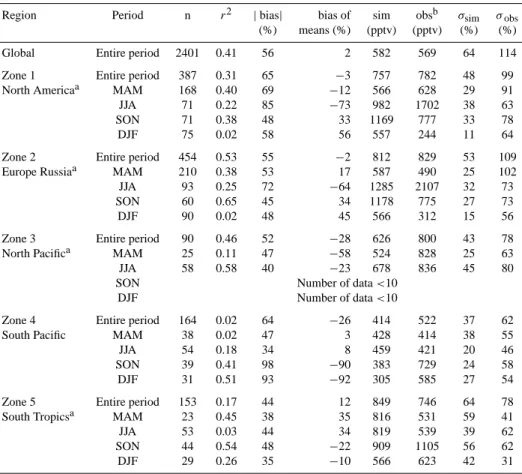
Table 1. Statistics derived from the comparison between observations and simulations at 8.5 km by season for different regions: n is the
number of data considered; (r2) the determination coefficient; | bias | is the average of the absolute values of the individual bias (simulation-observation in %); bias of means represents the bias between the mean values of the simulations and the (simulation-observations (%); sim and obs correspond to the mean vmr simulated and observed and σsimand σobsto their corresponding variability (rms).
Region Period n r2 |bias| bias of sim obsb σsim σobs (%) means (%) (pptv) (pptv) (%) (%) Global Entire period 2401 0.41 56 2 582 569 64 114 Zone 1 Entire period 387 0.31 65 −3 757 782 48 99 North Americaa MAM 168 0.40 69 −12 566 628 29 91 JJA 71 0.22 85 −73 982 1702 38 63 SON 71 0.38 48 33 1169 777 33 78
DJF 75 0.02 58 56 557 244 11 64
Zone 2 Entire period 454 0.53 55 −2 812 829 53 109 Europe Russiaa MAM 210 0.38 53 17 587 490 25 102 JJA 93 0.25 72 −64 1285 2107 32 73 SON 60 0.65 45 34 1178 775 27 73
DJF 90 0.02 48 45 566 312 15 56
Zone 3 Entire period 90 0.46 52 −28 626 800 43 78 North Pacifica MAM 25 0.11 47 −58 524 828 25 63 JJA 58 0.58 40 −23 678 836 45 80 SON Number of data <10
DJF Number of data <10
Zone 4 Entire period 164 0.02 64 −26 414 522 37 62 South Pacific MAM 38 0.02 47 3 428 414 38 55
JJA 54 0.18 34 8 459 421 20 46
SON 39 0.41 98 −90 383 729 24 58 DJF 31 0.51 93 −92 305 585 27 54 Zone 5 Entire period 153 0.17 44 12 849 746 64 78 South Tropicsa MAM 23 0.45 38 35 816 531 59 41
JJA 53 0.03 44 34 819 539 39 62
SON 44 0.54 48 −22 909 1105 56 62 DJF 29 0.26 35 −10 566 623 42 31
aNorth America: (50–80◦N; 180–40◦W)+(20–50◦N;130–40◦W);
Europe-Russia: (50–80◦N;20◦W–180◦E)+(35–50◦N;20◦W–140◦E); North Pacific: (0–60◦N; 140◦E–120◦W);
South Pacific: (60–0◦S; 150◦E–90◦W); South Tropics:(40–0◦S;20◦W–140◦E).
bWhen observed vmrs are averaged, the measurement noise is reduced (divided approximately by the square root of n). The resulting total
error (fitting + systematic) is then driven by the systematic error and is in the 20–30% range.
Table 2. Determination coefficients (r2) between methanol and two biomass burning tracers (CO and HCN), both measured by ACE-FTS. Region CH3OH/COa CH3OH/HCNa
JJA 2004 JJA 2005 JJA 2004 JJA 2005 North America (zone 1) 0.24 (−) 0.07 (+) 0.09 (−) 0.01 (−) Europe/Russia (zone 2) 0.30 (−) 0.12 (+) 0.28 (−) 0.14 (+) Imprint found in boreal plume 0.67 (+) −
Rinsland et al. (2007)
Imprint found in tropical plume 0.84 (+) 0.79 (+) Dufour et al. (2006)
aNegative and positive signs designate the sign of the correlation (r).
the Northern Pacific). This is in agreement with a continen-tal origin for the enhanced values observed. The seasonal
cycle of the methanol distribution observed for the northern latitudes (increase starting in spring for the midlatitudes and
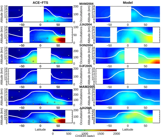
−50 0 50 6 8 10 12 14 16 18 ACE−FTS MAM2004 Altitude (km) −50 0 50 0 100 200 Occultations −50 0 50 6 8 10 12 14 16 18 Model Altitude (km) −50 0 50 6 8 10 12 14 16 18 JJA2004 Altitude (km) −50 0 50 0 50 100 Occultations −50 0 50 6 8 10 12 14 16 18 Altitude (km) −50 0 50 6 8 10 12 14 16 18 SON2004 Altitude (km) −50 0 50 0 100 200 Occultations −50 0 50 6 8 10 12 14 16 18 Altitude (km) −50 0 50 6 8 10 12 14 16 18 DJF2005 Altitude (km) −50 0 50 0 100 200 Occultations −50 0 50 6 8 10 12 14 16 18 Altitude (km) −50 0 50 6 8 10 12 14 16 18 MAM2005 Altitude (km) −50 0 50 0 100 200 300 Occultations −50 0 50 6 8 10 12 14 16 18 Altitude (km) −50 0 50 6 8 10 12 14 16 18 JJA2005 Latitude Altitude (km) CH3OH (pptv) −50 0 50 0 100 200 Occultations 0 500 1000 1500 2000 −50 0 50 6 8 10 12 14 16 18 Latitude Altitude (km)
Fig. 5. Zonal mean CH3OH volume mixing ratio profiles observed by the ACE-FTS (left) and simulated with the LMDz-INCA model (right)
for each season from March 2004 to August 2005. The modeled profiles used are interpolated at the measurement locations. The number of profiles averaged in each 20◦latitude band is indicated on the left panels (white squares). Only averages with more than 10 profiles are displayed. A mean tropopause height is calculated based on NCEP meteorological fields for each measured methanol profile and from the model for the calculated distributions (white line).
reaching a maximum for the highest latitudes in summer) fol-lows the seasonal cycle of the plant growth cycle and sug-gests that biogenic emissions drive the upper-tropospheric methanol concentration in the Northern Hemisphere. The large vmrs sampled over the Northern Atlantic reflect in-tercontinental transport. However, the northern hemispheric summer season is also the season of wildfires in the boreal regions and this can lead to large methanol concentrations in the upper troposphere (Rinsland et al., 2007). In order to separate the contribution of biogenic and biomass burning sources, we estimated the portions of the large vmrs mea-sured during JJA that are due to biomass burning. For this, we use the emission ratio of CH3OH with respect to CO
given by Andreae and Merlet (2001) and the CO vmr mea-sured by the ACE-FTS. A value of 90 ppbv is used as the background level of CO in the upper troposphere. All mea-surements in excess of this limit are considered to be the re-sult of biomass burning emissions. Figure 7 shows that about 25% of the measured methanol vmr could be due to these emissions in northern latitudes. For comparison, the biomass burning influence is greater than 60% in the tropics during
the biomass burning season (Fig. 7). We also calculated the coefficient of determination (r2) between CH3OH and CO
and HCN (two tracers of fire emissions) for North America and Europe-Russia (Table 2). These coefficients have to be compared to the correlation obtained inside boreal (Rinsland et al., 2007) and tropical (Dufour et al., 2006) plumes sum-marized in Table 2. Except for some specific measurements, Table 2 and Fig. 7 clearly indicate that biomass burning has a weak influence on the observed methanol in these regions. It confirms that biogenic emissions in the Northern Hemisphere are the major sources leading to large upper-tropospheric methanol values (as expected based on the partition of the total emissions displayed in Fig. 4).
4.2 Southern Hemisphere
In the Southern Hemisphere, the seasonal variation is fairly weak since most of the land masses are located in the trop-ics where the seasonal cycle of the vegetation and hence of biogenic emissions is weak. However, the satellite measurements show the clear influence of biomass burning
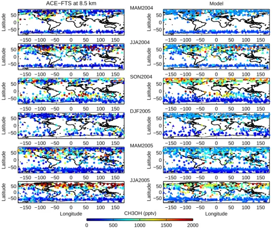
−150 −100 −50 0 50 100 150 −50 0 50 ACE−FTS at 8.5 km MAM2004 Latitude −150 −100 −50 0 50 100 150 −50 0 50 Model Latitude −150 −100 −50 0 50 100 150 −50 0 50 JJA2004 Latitude −150 −100 −50 0 50 100 150 −50 0 50 Latitude −150 −100 −50 0 50 100 150 −50 0 50 SON2004 Latitude −150 −100 −50 0 50 100 150 −50 0 50 Latitude −150 −100 −50 0 50 100 150 −50 0 50 DJF2005 Latitude −150 −100 −50 0 50 100 150 −50 0 50 Latitude −150 −100 −50 0 50 100 150 −50 0 50 MAM2005 Latitude −150 −100 −50 0 50 100 150 −50 0 50 Latitude 0 500 1000 1500 2000 −150 −100 −50 0 50 100 150 −50 0 50 JJA2005 Longitude Latitude CH3OH (pptv) −150 −100 −50 0 50 100 150 −50 0 50 Longitude Latitude
Fig. 6. Methanol volume mixing ratios at 8.5 km height observed by the ACE-FTS (left) and simulated by LMDz-INCA (right) for each
season from March 2004 to August 2005. Squares, circles and triangles represent the first, second and the third month of the period, respectively. The modeled vmrs at 8.5 km are interpolated at the measurement locations.
emissions on the methanol distribution in the tropics. This is particularly the case during March-April-May (MAM) and September-October-November (SON) 2004 with zonally-averaged vmrs up to 1200 pptv (Fig. 5). Biomass burning plumes with methanol vmrs reaching more than 2000 pptv and emanating from southern Africa and South America, and detected over the Indian and southern Atlantic oceans are also clearly seen in SON during the peak burning sea-son in the Southern Hemisphere (Fig. 6). In this case, the part of the methanol concentration due to biomass burning is greater than 60% (Fig. 7). The biomass burning origin of these plumes is also confirmed by the positive correlation ob-served between methanol and both CO and HCN, two tracers of biomass burning emissions in the atmosphere (Dufour et al., 2006; Rinsland et al., 2005).
5 Comparison with the LMDz-INCA CTM
In order to test our knowledge of the methanol budget, the observations are compared to the simulations of the LMDz-INCA CTM in Figs. 5 and 6 and in Table 1. For com-parison with the ACE occultations, the simulated daily
av-eraged methanol profiles are interpolated to the measure-ment locations. The interpolation is bilinear in latitude and longitude and only the days with measurements are consid-ered. We checked that the resulting model results (and es-pecially the seasonal and monthly means) were representa-tive of the entire model results (i.e., when all the grid cells and all the days of the considered season are included in the means). The agreement between observations and simula-tions is rather encouraging on a global scale considering the large uncertainties in surface emissions. The bias between the mean measured and simulated vmrs at 8.5 km for the en-tire period studied (March 2004 to August 2005) is only 2%. This is to be considered relative to the errors in the retrieved methanol values that are about 20–30% when data are av-eraged. However, the correlation coefficient (0.41) and the absolute bias (56%, Table 1) reveal compensating effects on the average. Furthermore, the variability of the measured methanol is much larger than the modeled variability of the measurements (Table 1). The lack of variability is usual with global scale models and is mainly due to the coarse resolution of the model that does not allow individual events to be de-scribed. In the following, we show that, although the model simulates rather reasonably the average features of CH3OH
Fig. 7. Portion (%) of the measured CH3OH vmrs at 8.5 km due
to biomass burning source averaged over 10◦-latitude bands for the seasons potentially affected. This portion is calculated using the emission ratio of methanol with respect to CO given by Andreae and Merlet (2001), the CO vmrs measured by the ACE-FTS, and a limit of 90 ppbv for background CO.
(considering uncertainties in the measurements and the emis-sions), the model has difficulties in reproducing the seasonal cycle observed in the Northern Hemisphere.
A general point also to note on the model performance is how the profile shape (especially in the lower stratosphere) compares between the model and the observations. The model does not reproduce the rapid decrease with height ob-served by ACE-FTS above the tropopause (Fig. 5) and the model results overestimate the measurements by 70% in the lower stratosphere. The degree of overestimation has to be considered carefully because of the large uncertainties in the observations above the tropopause. However, two reasons can explain this apparent disagreement: (i) the model is de-signed for tropospheric studies and the coarse resolution in the stratosphere and upper troposphere does not permit the reproduction of the variation observed; (ii) vertical transport remains subject to large uncertainties in such global models in particular regarding large scale convection or stratospheric intrusion. Hauglustaine et al. (2004) also pointed out that the model is too diffusive which is visible in Fig. 5: the gradient across the tropopause is smaller than that observed and may lead to a lack of methanol in the upper troposphere. This has to be kept in mind in the following discussion.
5.1 Northern Hemisphere
Despite a fair general agreement between the model and the measurements, a seasonal comparison reveals some dis-crepancies that we attribute mainly to a misrepresentation of some emission sources. Figure 5 illustrates the strong un-derestimation of upper tropospheric methanol by the model during summer when the influence of biogenic sources on the measured vmr is large at northern mid-to-high latitudes. Dur-ing the Northern Hemisphere summer (JJA), the simulated
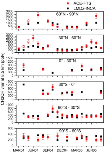
Fig. 8. Monthly variations of measured (red) and simulated (black)
mixing ratios at 8.5 km averaged for 30◦-latitude bands. The symbols are open when the number of available measurements is smaller than 10. A total error estimate of 20% is considered for all the latitude bands except the 90◦S-60◦S band, for which a total error estimate of 30% is retained (smaller vmrs in this band).
mixing ratios are only 60% of the measured values at the maximum of the profile for latitudes higher than 50◦N. This disagreement arises mostly from continental regions (Fig. 6). Measured methanol values over the continents in the North-ern Hemisphere are much larger than the simulated values (e.g., up to 73% over North America) whereas they are in bet-ter agreement over the oceans considering the measurement errors (North Pacific: 23%) (Table 1). A summer continen-tal source that can lead to enhancement of methanol mixing ratios in the high latitudes is boreal fires. As Fig. 7 shows, the contribution of biomass burning to the measured vmrs is of the order of the errors of the measurements. The dis-agreement, therefore, between observations and simulations during the northern hemispheric summer points towards an underestimate of methanol biogenic emissions and this is also true during the plant growth phase in spring. As Fig. 6 shows, large methanol concentrations are measured in April
and May for the mid-latitudes whereas the model does not reproduce these enhanced values. This spring underestima-tion is not completely obvious looking at the bias in Table 1. This is mainly due to the sampling of the data which is pri-marily at high latitude for March and is sparser in April-May for the mid-latitudes. A compensation effect then oc-curs while averaging over the three months, especially since the March values seem overestimated by the model during winter. To test the hypothesis of the underestimation of the simulated methanol during spring and summer, an additional model run was performed with biogenic emissions increased by 50% (not shown). In this case, the disagreement is signif-icantly reduced over land in spring and summer. Most of the large methanol values observed in May over North America and Europe-Russia are well represented by the model. The bias between the mean vmrs and the absolute bias during JJA over North America are much reduced to about 9%, which is within the error of the measurements (20–30% when consid-ering averages), and to 41% compared to 85%, respectively. However, the differences between the observations and the simulations are increased for the other seasons in this addi-tional model run.
Another important difference between the simulations (reference case) and the observations arising in the Northern Hemisphere is that the modeled upper-tropospheric methanol peaks in fall especially for the highest latitudes whereas mea-surements and emissions peak in summer (Figs. 5 and 6). The model overestimates observed methanol by about 35% for both North America and Europe-Russia (Table 1). In or-der to investigate in detail these disagreements on the inten-sity and the seasonality of the upper-tropospheric methanol cycle, the monthly variations of methanol measured and sim-ulated at 8.5 km are displayed for 30◦latitude bands in Fig. 8.
Notice that the underestimation of methanol during spring and summer starting in April is also very obvious in this fig-ure. The model overestimation identified during the SON period is essentially due to an overestimation in October and November. Moreover, above the Northern Hemisphere con-tinents, the winter methanol values are overestimated by the model even if we account for the errors of about 30% on the mean measured methanol (Table 1). Considering only the deposition and the chemical sinks of methanol (not the transport), we estimate a lifetime of about 69 days for the months of October, November and December in the 60– 90◦N latitude band. This long lifetime would explain the persistence of relatively large methanol values in the model for these latitudes during winter. The overestimation of the model would suggest that the simulated OH amounts are not sufficient during winter. This latter assumption is difficult to check because very little information is available on the upper-tropospheric OH distribution. Only climatological val-ues are available (Spivakovsky et al., 2000) and show that there is very little OH during winter for these latitudes. An-other hypothesis for the model overestimation is that depo-sition is underestimated. This hypothesis is also difficult to
check because of the uncertainty in the methanol deposition. Depending on the studies, the estimation of this sink varies by as much as a factor of 2 (Jacob et al., 2005, Table 1). A misrepresentation of the transport in the model, in particu-lar the diffusion, combined with the above hypothesis, could also contribute to the accumulation of large methanol con-centrations in the high latitudes in the simulations.
5.2 Southern Hemisphere
For the Southern Hemisphere, the observations show that the major component of the emissions that imposes a seasonal variation on upper tropospheric methanol are the biomass burning emissions and their transport over oceans (Indian and South Pacific), especially during the SON period (Fig. 6). This is easily visible in October in the monthly variations for the 0-30◦S and 30–60◦S latitude bands in Fig. 8. The south
tropical region defined in Table 1 (zone 5) is the most af-fected by biomass burning emissions with a maximum during the SON period (Fig. 5 and 6). The model reproduces with some accuracy the high methanol levels measured in this re-gion (within the estimated errors). During the other seasons, the agreement is also rather good with a tendency to overesti-mate methanol. In JJA, the modeled values are larger than the observed ones mainly over South America and are likely due to biomass burning emissions included in the model (Fig. 6). This would suggest that these emissions are overestimated. In MAM2005, the average of modeled methanol vmrs is increased only by two occultations that can be considered as outliers (Fig. 6). Upper-tropospheric methanol measured above South Pacific during SON2004 is also affected by biomass burning and especially by the long-range transport of biomass burning plumes. The model has some difficulties in reproducing the observed values (Table 1). This is likely an effect of the resolution of the global model and thus of the representivity of the model compared to the measurements. This leads to a dilution of the plume influence in each model grid area and therefore does not permit a precise description of the transport and chemical evolution inside a plume. On another hand, the underestimation of the model observed in DJF2005 is due to the relatively large values measured down-wind of Australia and might reflect an underestimation of the Australian biogenic emissions during the austral summer. Moreover, looking in detail Fig. 6 shows that the ACE-FTS is also able to detect a strong signature from pollution sources in the upper troposphere. The satellite measurements reveal large methanol concentrations above China and India dur-ing MAM 2005. These enhanced values are reproduced by the model but to a much lesser extent. This disagreement points to underestimated anthropogenic emissions of hydro-carbons in currently available emission inventories over these regions, a conclusion also reached by other studies for car-bon monoxide (Kasibhatla et al., 2002; Heald et al., 2004; P´etron et al., 2002). Finally, the comparison between the model and the measurements for the high southern latitudes
is fairly good and is largely within the observation errors. The methanol measured and simulated in these regions is not influenced by any continental sources and reflects the atmo-spheric background.
6 Conclusions
Global measurements from a space-borne infrared limb-viewing instrument can measure the height-resolved distri-bution of methanol in the mid and upper troposphere. These measurements provide a unique view of the pervasive influ-ence of biogenic emissions on the composition of the upper troposphere at northern mid and high latitudes. Furthermore, the satellite observations reveal how the upper troposphere is directly affected by surface and lower-tropospheric pro-cesses. The integration of these global methanol measure-ments from space with model results and airborne observa-tions should significantly improve our understanding of the atmospheric budget of this important oxygenated species and the role played by the vegetation as a source of chemical species. It should also help to improve model simulations in future studies. The measured profiles will also help to bet-ter quantify the role played by methanol as a major source of radicals in the upper troposphere.
Acknowledgements. The ACE mission is funded by the Canadian
Space Agency and the Natural Sciences and Engineering Research Council of Canada. NCEP Reanalysis data provided by the NOAA/OAR/ESRL PSD, Boulder, Colorado, USA, from their Web site at http://www.cdc.noaa.gov.
Edited by: P. Monks
References
Andreae, M. O. and Merlet, P.: Emission of trace gases and aerosols from biomass burning, Global Biogeochem. Cy., 15, 955–966, 2001.
Bernath, P. F., McElroy, C. T., Abrams, M. C., Boone, C. D., Butler, M., Camy-Peyret, C., Carleer, M., Clerbaux, C., Coheur, P.-F., Colin, R., DeCola, P., DeMazi`ere, M., Drummond, J. R., Dufour, D., Evans, W. F. J., Fast, H., Fussen, D., Gilbert, K., Jennings, D. E., Llewellyn, E. J., Lowe, R. P., Mahieu, E., McConnell, J. C., McHugh, M., McLeod, S. D., Michaud, R., Midwinter, C., Nas-sar, R., Nichitiu, F., Nowlan, C., Rinsland, C. P., Rochon, Y. J., Rowlands, N., Semeniuk, K., Simon, P., Skelton, R., Sloan, J. J., Soucy, M.-A., Strong, K., Tremblay, P., Turnbull, D., Walker, K. A., Walkty, I., Wardle, D. A., Wehrle, V., Zander, R., and Zou, J.: Atmospheric Chemistry Experiment (ACE): mission overview, Geophys. Res. Lett., 32, L15S01, doi:10.1029/2005GL022386, 2005.
Bernath, P. F.: Atmospheric Chemistry Experiment (ACE): Analyti-cal chemistry from orbit, Trends AnalytiAnalyti-cal Chem., 25, 647–654, 2006.
Boone, C. D., Nassar, R., Walker, K. A., Rochon, Y., McLeod, S. D., Rinsland, C. P., and Bernath, P. F.: Retrievals for the
at-mospheric chemistry experiment Fourier-transform spectrome-ter, Appl. Opt., 44, 7218–7231, 2005.
Dufour, G., Boone, C. D., Rinsland, C. P., and Bernath, P. F.: First space-borne measurements of methanol inside aged south-ern tropical to mid-latitude biomass burning plumes using the ACE-FTS instrument, Atmos. Chem. Phys., 6, 3463–3470, 2006, http://www.atmos-chem-phys.net/6/3463/2006/.
Folberth, G. A., Hauglustaine, D. A., Lathi`ere, J., and Rocheton, F.: Interactive chemistry in the Laboratoire de M´et´eorologie Dy-namique general circulation model: model description and im-pact analysis of biogenic hydrocarbons on tropospheric chem-istry, Atmos. Chem. Phys., 6, 2273–2319, 2006,
http://www.atmos-chem-phys.net/6/2273/2006/.
Fu, D., Boone, C. D., Bernath, P. F., Walker, K. A., Nassar, R., Man-ney, G. L., and McLeod, S. D.: Global phosgene observations from the Atmospheric Chemistry Experiment (ACE) mission, Geophys. Res. Lett., 34, L17815, doi:10.1029/2007GL029942, 2007.
Galbally, I. E. and Kristine, W.: The production of methanol by flowering plants and the global cycle of methanol, J. Atmos. Chem., 43, 195–229, 2002.
Hauglustaine, D. A., Hourdin, F., Jourdain, L., Filiberti, M.-A., Walters, S., Lamarque, J.-F., and Holland, E. A.: Interac-tive chemistry in the Laboratoire de M´et´eorologie Dynamique general circulation model: Description and background tropo-spheric chemistry evaluation, J. Geophys. Res., 109, D04314, doi:10.1029/2003JD003957, 2004.
Heald, C. L., Jacob, D. J., Jones, D. B. A., Palmer, P. I., Logan, J. A., Streets, D. G., Sachse, G.W., Gille, J. C., Hoffman, R. N., and Nehrkorn, T.: Comparative inverse analysis of satellite (MO-PITT) and aircraft (TRACE-P) observations to estimate Asian sources of carbon monoxide, J. Geophys. Res., 109, D23306, doi:10.1029/2004JD005185, 2004.
Heikes, B., Chang, W., Pilson, M. E. Q., Swift, E., Singh, H. B., Guenther, A., Jacob, D. J., Field, B. D., Fall, R., Riemer, D., and Brand, L.: Atmospheric methanol budget and ocean implication, Global Biogeochem. Cy., 16(4), 1133, doi:10.1029/2002GB001895, 2002.
Jacob, D. J., Field, B. D., Li, Q., Blake, D. R., de Gouw, J., Warneke, C., Hansel, A., Wisthaler, A., Singh, H. B., and Guenther, A.: Global budget of methanol: Constraints from atmospheric observations, J. Geophys. Res., 110, D08303, doi:10.1029/2004JD005172, 2005.
Karl, T., Guenther, A., Spirig, C., Hansel, A., and Fall, R.: Sea-sonal variation of biogenic VOC emissions above a mixed hard-wood forest in northern Michigan, Geophys. Res. Lett., 23, 2186, doi:10.1029/2003GL018432, 2003.
Kasibhatla, P., Arellano, A., Logan, J. A., Palmer, P. I., and Novelli, P.: Top-down estimate of a large source of atmospheric carbon monoxide associated with fuel combustion in Asia, Geophys. Res. Lett., 29, 1900, doi:10.1029/2002GL015581, 2002. Lathi`ere, J., Hauglustaine, D. A., De Noblet-Ducoudr´e, N.,
Krin-ner, G., and Folberth, G. A.: Past and future changes in biogenic volatile organic compound emissions simulated with a global dynamic vegetation model, Geophys. Res. Lett., 32, L20818, doi:10.1029/2005GL024164, 2005.
Lathi`ere, J., Hauglustaine, D. A., Friend, A. D., De Noblet-Ducoudr´e, N., Viovy, N., and Folberth, G. A.: Impact of climate variability and land use changes on global biogenic volatile
or-ganic compound emissions, Atmos. Chem. Phys., 6, 2129–2146, 2006,
http://www.atmos-chem-phys.net/6/2129/2006/.
P´etron, G., Granier, C., Khattatov, B., Lamarque, J.-F., Yudin, V., M¨uller, J.-F., and Gille, J.: Inverse modeling of carbon monox-ide surface emissions using Climate Monitoring and Diagnostics Laboratory network observations, J. Geophys. Res., 107, 4761, doi:10.1029/2001JD001305, 2002.
Rinsland, C. P., Dufour, G., Boone, C. D., Bernath, P. F., and Chiou, L.: Atmospheric Chemistry Experiment (ACE) measure-ments of elevated Southern Hemisphere upper tropospheric CO, C2H6, HCN, and C2H2 mixing ratios from biomass burning emissions and long-range transport, Geophys. Res. Lett., 32, L20803, doi:10.1029/2005GL024214, 2005.
Rinsland, C. P., Dufour, G., Boone, C. D., Bernath, P. F., Chiou, L., Coheur, P-F., Turquety, S., and Clerbaux, C.: Satellite bo-real measurements over Alaska and Canada during June-July 2004: simultaneous measurements of upper tropospheric CO, C2H6, HCN, CH3Cl, CH4, C2H2, CH3OH, HCOOH, OCS, and SF6 mixing ratios, Global Biogeochem. Cy., 21, GB3008, doi:10.1029/2006GB002795, 2007.
Schade, G. W. and Goldstein, A. H.: Seasonal measurements of acetone and methanol: Abundances and implications for atmospheric budgets, Global Biogeochem. Cy., 20, GB1011, doi:10.1029/2005GB002566, 2006.
Singh, H. B., Kanakidou, M., Crutzen, P. J., and Jacob, D. J.: High concentrations and photochemical fate of oxygenated hydrocar-bons in the global troposphere, Nature, 378, 50–53, 1995. Singh, H. B., Chen, Y., Tabazadeh, A., Fukui, Y., Bey, I.,
Yan-tosca, R., Jacob, D., Arnold, F., Wohlfrom, K., Atlas, E., Flocke, F., Blake, D., Blake, N., Heikes, B., Snow, J., Talbot, R., Gre-gory, G., Sachse, G., Vay, S., and Kondo, Y.: Distribution and fate of selected oxygenated organic species in the troposphere and lower stratosphere over the Atlantic, J. Geophys. Res., 105, 3795–3805, 2000.
Singh, H. B, Chen, Y., Staudt, A., Jacob, D., Blake, D., Heikes, B., and Snow, J.: Evidence from the Pacific troposphere for large global sources of oxygenated organic compounds, Nature, 410, 1078–1081, 2001.
Singh, H. B., Tabazadeh, A., Evans, M. J., Field, B. D., Jacob, D. J., Sachse, G., Crawford, J. H., Shetter, R., and Brune, W. H.: Oxygenated volatile organic chemicals in the oceans: In-ferences and implications based on atmospheric observations and air-sea exchange models, Geophys. Res. Lett., 30, 1862, doi:10.1029/2003GL017933, 2003.
Singh, H. B., Salas, L. J., Chatfield, R. B., Czech, E., Fried, A., Walega, J., Evans, M. J., Field, B. D., Jacob, D. J., Blake, D., Heikes, B., Talbot, R., Sachse, G., Crawford, J. H., Avery, M. A., Sandholm, S., and Fuelberg, H.: Analy-sis of the atmospheric distribution, sources, and sinks of oxy-genated volatile organic chemicals based on measurements over the Pacific during TRACE-P, J. Geophys. Res., 109, D15S07, doi:10.1029/2003JD003883, 2004.
Sinha, V., Williams, J., Meyerh¨ofer, M., Riebesell, U., Paulino, A. I., and Larsen, A.: Air-sea fluxes of methanol, acetone, acetalde-hyde, isoprene and DMS from a Norwegian fjord following a phytoplankton bloom in a mesocosm experiment, Atmos. Chem. Phys., 7, 739–755, 2007,
http://www.atmos-chem-phys.net/7/739/2007/.
Spivakovsky, C. M., Logan, J. A., Montzka, S. A., Balkanski, Y. J., Foreman-Fowler, M., Jones, D. B. A., Horowitz, L. W., Fusco, A. C., Brenninkmeijer, C. A. M., Prather, M. J., Wofsy, S. C., and McElroy, M. B.: Three-dimensional climatological distribution of tropospheric OH: Update and evaluation, J. Geophys. Res., 105, 8931–8980, 2000.
Tie, X., Guenther, A., and Holland, E.: Biogenic methanol and its impacts on tropospheric oxidants, Geophys. Res. Lett., 30, 1881, doi:10.1029/2003GL017167, 2003.
van der Werf, G. R., Randerson, J. T., Collatz, G. J., Giglio, L., Kasibhatla, P. S., Arellano, A. F., Olsen, S. C., and Kasischke, E. S.: Continental-scale partitioning of fire emissions during the 1997 to 2001 El Nino/La Nina period, Science, 303(5654), 73– 76, 2004.
Von Kuhlmann, R., Lawrence, M. G., Crutzen, P. J., and Rasch, P. J.: A model for studies of tropospheric ozone and nonmethane hy-drocarbons: Model evaluation of ozone–related species, J. Geo-phys. Res., 108, 4729, doi:10.1029/2002JD003348, 2003.