Comparison of statistical and artificial neural network techniques for estimating past sea surface temperatures from planktonic foraminifer census data

HAL Id: hal-02916209

https://hal.archives-ouvertes.fr/hal-02916209

Submitted on 9 Oct 2020

HAL is a multi-disciplinary open access

archive for the deposit and dissemination of

sci-entific research documents, whether they are

pub-lished or not. The documents may come from

teaching and research institutions in France or

abroad, or from public or private research centers.

L’archive ouverte pluridisciplinaire HAL, est

destinée au dépôt et à la diffusion de documents

scientifiques de niveau recherche, publiés ou non,

émanant des établissements d’enseignement et de

recherche français ou étrangers, des laboratoires

publics ou privés.

Comparison of statistical and artificial neural network

techniques for estimating past sea surface temperatures

from planktonic foraminifer census data

Björn A. Malmgren, Michal Kucera, Johan Nyberg, Claire Waelbroeck

To cite this version:

Björn A. Malmgren, Michal Kucera, Johan Nyberg, Claire Waelbroeck. Comparison of statistical

and artificial neural network techniques for estimating past sea surface temperatures from planktonic

foraminifer census data. Paleoceanography, American Geophysical Union, 2001, 16 (5), pp.520-530.

�10.1029/2000PA000562�. �hal-02916209�

PALEOCEANOGRAPHY, VOL. 16, NO. 5, PAGES 520-530, OCTOBER 2001

Comparison of statistical and artificial neural network techniques for

estimating past sea surface temperatures from planktonic foraminifer

census data

Bj6m A. Malmgren,

• Michal

Kucera,

2 Johan

Nyberg,

• and Claire

Waelbroeck

3

Abstract. We present the first detailed and rigorous comparison of six different computational techniques used to

reconstruct

sea surface temperatures

(SST) from planktonic foraminifer census data. These include the Imbrie-Kipp

transfer functions (IKTF), the modem analog technique (MAT), the modem analog technique with similarity index

networks (ANN) trained on a large faunal data set, including a modification

where geographical

information

was added

among the input variables (ANND). By training the techniques on an identical database, we were able to explore the

differences in SST reconstructions resulting solely from the use of different mathematical methods. The comparison

indicates that while the IKTF technique consistently shows the worst performance, ANN and RAM perform slightly

better than MAT and that the inclusion of the geographical information into the training database (SIMMAX and ANND)

further improves the accuracy of modem SST estimates. However, when applied to an independent validation data set

and an additional fossil data set, the results did not conform to this ranking. The largest differences in the reconstructed

SST values occurred between groups of techniques with different approaches to SST reconstruction; that is, ANN and

ANND produced SST reconstructions

significantly different from those produced

by RAM, SIMMAX, and MAT. The

application of the various techniques to the validation data set, which allowed comparison of SST reconstructions with

instrumental records, suggests that artificial neural networks might provide better paleo-SST estimates than the other

techniques.

1. Introduction

One of the most remarkable consequences of Charles Lyell's uniformitarian principle for the field of paleoceanography has been the opportunity to use the relationship between the distribution of modem faunas and floras and present-day physical conditions in the ocean to reconstruct climatic variations in the Quaternary period. In addition, if this relationship were expressed in the form of a mathematical formula, past climatic variations could be quantified in standard physical scales and units. This appealing prospect was discovered early in paleoceanographical studies, and quantitative reconstruction of Quaternary climate change by means of fossil faunas has become a standard and routinely applied procedure.

Some early attempts at quantifying the relationship between species abundances and observed physical parameters relied on relatively simple mathematical methods [see Hutson, 1977]. The straggle for improvement in the precision of the estimates caused researchers to resort to more complex, often computer- intensive, statistical methods. To date, three different approaches have been used to quantify the relationship between faunal data and physical properties of the environment. The first approach, known as the Imbrie-Kipp transfer function (IKTF) method [Imbrie and Kipp, 1971], utilizes the standard statistical techni- que of Q mode principal component analysis to decompose the

•Department of Earth Sciences--Marine Geology, Earth Sciences

Centre, G6teborg University, G6teborg, Sweden.

2Department of Geology, Royal Holloway College, University of London, Egham, Surrey, England, United Kingdom.

3Laboratoire des Sciences du Climat et de l'Environnement, Laboratoire

Mixte CNRS-CEA, Domaine du CNRS, Gif-sur-Yvette, France.

Copyright 2001 by the American Geophysical Union.

Paper number 2000PA000562.

0883-8305/01/2000PA000562512.00

variation in the faunal data into a smaller number of variables that are then regressed upon the known physical parameters. Hutson [1980] developed an alternative approach: His modem analog technique (MAT) does not generate a unique calibration formula between faunal data and physical properties. Instead, this method searches the database of modem faunas for samples with assemblages that most resemble the fossil assemblage. The envi- ronment representing the fossil sample is then reconstructed from the physical properties recorded in the best modem analog sam- ples. While the IKTF approach relies upon the assumption that the reconstruction of species' responses to physical parameters will yield the most reliable estimates of past environments, MAT, a true incarnate of Lyell's uniformitarianism, resorts solely to searching

for modem situations most similar to that observed in a fossil

sample. Significant improvements of this approach include the modem analog with similarity index (SIMMAX) method [Pfiau- mann e! al., 1996] and the revised analog method (RAM) [14/ael- broeck et al., 1998].

The third approach, using artificial neural networks (ANN), a branch of artificial intelligence, relies on the sole assumption that there, indeed, is a relationship between the distribution of modem faunas and the physical properties of the environment. ANNs have the ability to overcome problems of fuzzy and nonlinear relationships between sets of input and output variables. This computer-intensive approach is based on an algorithm that has the ability of autonomous "learning" of a relationship between two groups of numbers [14/assetman, 1989; Beale and Jackson, 1990]. Once trained, the neural network serves as a unique transfer function, yet at the same time this highly nonlinear and recurrent function is so complex that it has the ability to simulate a decision algorithm. The utility of ANN in reconstructing past environmental conditions has been recently demonstrated by Malmgren and Nordlurid [ 1997].

The existence of different approaches to sea surface temperature (SST) reconstruction inevitably raises questions of whether there 520

MALMGREN ET AL.: ESTIMATING PAST SEA SURFACE TEMPARATURES 521

2. Material and Methods

• 0 o

(30 ø 2.1. Calibration Data Set

As the basis for the training and performance analysis, census counts of planktonic foraminifera in 740 core tops from the

1•l.l•2•,•l•l.?,

•

Atlantic

Ocean

(latitudinal

range

87øN-40øS)have

been

used.

PFI

compiled

by Pfiaumann

et al. [ 1996]

and

two

additional

core

tops

from the Caribbean Sea (Figure 1 and Table 1), which were

40ø included

in order

to increase

the

coverage

of the

tropical

Atlantic

database.

•

5--...f.

The

census

counts

of planktonic

foraminifera

in the

two

addi-

••o

-

...

tional

samples

were

generated

in

the

same

way

as

those

in

the

• ,•,•

120ø

databaseøfPfiaumannetal'

[1996]'Thecøuntswerebasedøn

•-'

gories

of planktonic

foraminifera

were

quantified

in each

sample

0

ø using

the

same

criteria

as

Pfiaumann

et

al.

[ 1996].

Box

core

PRB-

Pb-210 and Cs-137 methods at Riso National Laboratory, Ros- kilde, Denmark [Nyberg et al., 2001]. The results indicate a

relatively

uniform

sedimentation

rate between

3 and 4 mm yr -•

-20 ø -20 ø throughout the top 15 cm of the core. Each 1-cm-thick interval

-80 ø

-60 ø

-40 ø

-20 ø

0 ø

should

thus

represent

•3 years.

Therefore

the 1-cm-thick

core

top

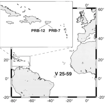
Figure 1. Location of the two Caribbean core tops (PRB-7 and PRB-12) added to the database used by Pfiaumann et al. [1996].

The box core PRB- 12 was used for the validation of the sea surface

temperature (SST) prediction techniques. Also shown is the location of core V 25-59, which was used to examine the differences among the techniques when applied to a fossil data set.

are significant differences among the SST estimates produced by these techniques, how these differences can be explained, and what is the potential influence of the techniques on the validity of the SST estimates. This issue is of great importance since census count-based SST estimates provide the only nongeochemical, and thus truly independent, palcothermometer. Previous attempts to answer these questions have either concentrated only on two of the then available techniques [Prell, 1985; Le, 1992; Ortiz and Mix, 1997] or have presented comparisons of limited statistical validity (different training sets [Waelbroeck et al., 1998] and a small training set [Maimarch and Nordlund, 1997]).

Here we present a detailed and rigorous evaluation of the efficacy of six different techniques used to reconstruct the relation- ship between modem faunas and SST data, including for the first time a set of ANNs trained on a large faunal data set. The comparison is based on planktonic foraminifer census counts from the Atlantic core top database of Pfiaumann et al. [1996], which includes data generated by Climate: Long-Range Investigation, Mapping, and Prediction Project Members [1984]. We compare the performance of the techniques for estimating modem SSTs, and we show the discrepancies among these techniques when applied to independent data, both from recent times, with known temper- ature variations, and from a Late Pleistocene core with a presum- ably larger amount of no-analog assemblages.

should span an interval between December 1994, when the cores

were recovered, and the fall of 1991. We assume that the sed- imentation rate in box core PRB-07 was similar; both cores are

located <1 km from each other (Table 1).

For the purpose of calibration, "measured" SST data of Pfiau- mann et al. [ 1996] were used for both caloric seasons. Throughout this paper, "warm season" SST represents the mean for August- October, while "cold season" SST represents the mean for February-April (and conversely in the Southern Hemisphere). The SST values of Pfiaumann et al. [1996] have been extracted from the database of Levitus [1982], which summarizes SST observations over some 100 years and is thus appropriate for the assignment of SST values to deep-sea core top samples. We have used the mean temperature for 0- to 75-m water depth as a representation of the SST, as Pfiaumann et al. [ 1996] showed that this yields the least standard deviation of SST residuals.

The SSTs for the Caribbean core tops were calculated as arithmetic means of the corresponding temperatures between 1991 and 1994. The temperatures for 1991 - 1992 were taken from the Comprehensive Ocean-Atmosphere Data Set (COADS) grid of

2 ø by 2 ø (node at 67øW, 17øN); for 1992-1994 we used the data

from da Silva et al. [1994]. Both databases list the SST without specification of the depth range. At present, the Levims [1982] 0- to 75-m SST and the 0- to 5-m SST off Puerto Rico differ for the warm season by •0.4øC, and for the cold season they differ by -0.1 øC (Figure 2). In comparison with the 1991-1994 data, the 0- to 5-m SST from Levims [1982] is the same for the warm season, while for the cold season the long-term average is cooler by

•0.2øC (Figure 2).

2.2. Validation Data Set and Fossil Data Set

The most appropriate way to determine the accuracy of SST reconstructions produced by different techniques is through a

Table 1. Data on the Two Cores Added to the Core Top Database Compiled by Pfiaumann et al. [1996] a

Water Depth, Latitude, Longitude, Dating WS SST, CS SST,

Core m øN øW øC øC N

PRB-7 273 17052.82 ' 66035.90 ' NA 28.52 26.60 382

PRB- 12 360 17ø53.27' 66036.02 ' Pb-210 28.52 26.60 334

aBoth cores were taken off the coast of Puerto Rico in December 1994. Abbreviations are as follows: WS, warm season; SST, sea surface

522 MALMGREN ET AL.: ESTIMATING PAST SEA SURFACE TEMPARATURES 29.0 28.5 28.0 0 27.5 o (,,J) 27.0 26.5 26.0 25.5 I Jan 1991-1994 "surface" • 28.53oc

-- Levitus

[1982]

0

m

m 28.52o0/-?•½...

/m

S.eason •/

Warm

Feb Mar Apr May Jun Jul Aug Sep Oct Nov Dec

Month

Figure 2. Average seasonal SST variation off Puerto Rico (square grid node at 67øW, 17øN) at different water

depths (data from Levitus [ 1982]). The long-term warm season and cold season averages for 0-m and 0- to 75-m water

depths are shown together with the corresponding values for 1991-1994 taken from the Comprehensive Ocean-

Atmosphere Data Set (COADS) and da Silva et al. [1994]. In winter the water column is relatively homogenous,

while in summer the surface layer (0-5 m) is warmer by •0.4øC than the average temperature for the entire upper 0-

to 75-m layer.

validation of estimates from an independent set of samples with known SST values. The variability of the validation data set should resemble faunal variation in fossil assemblages. For the purpose of

such validation we have selected the Caribbean box core PRB-12

(Table 1). On the basis of Pb-210 and Cs-137 dating [Nyberg et al., 2001] the top 15 cm of this box core span the last 50 years (•1945-1994), thus allowing us to compare the estimated SSTs with historical records (COADS and da Silva et al. [1994]). The age model for the top 15 cm of the core is based on measurements of Pb-210 activity in 12 samples and Cs-137 activity in 14 samples. The error of the age model due to measurement uncertainties is <10% (i.e., <5 years) for all samples. It should be noted that SST in this data set is defined as "sea surface" temperature, while the prediction techniques are being calibrated on a data set where SST is defined as the mean from 0- to 75-m water depth. Thus, as discussed in section 2.1, because of this discrepancy we may

expect a consistent offset of •0.4øC between the predicted and

the observed SST for the warm season estimates (Figure 2). Eight 1-cm-thick samples were taken every 2 cm from the top 15 cm of the box core. In each sample, planktonic foraminifer census data were generated by counting between 287 and 430 specimens. No signs of calcite dissolution were observed, which was con- firmed by low percentages of planktonic foraminifer fragments in all samples. The major drawback of core PRB-12 is that it derives from an area where SSTs are at the warm end of the SST range in the training data set.

Planktonic foraminifer census data from the low-latitude core V

25-59 (Figure 1, 1ø22'N, 33ø29'W) were used to assess

the

differences in SST reconstructions among the techniques when applied to this fossil data set, presumably containing many no- analog samples. The original data set by Mcintyre et al. [1989],

' ø ø •..1!

COh,v,•h,• 45 spcc•cs flllU "*"• species groups, •v,• •,,,ed to include only the taxonomic categories used in the database ofPfiaumann et al. [ 1996]. The faunal variation during the last • 150 kyr recorded in the upper 400 cm of this core has been the subject of extensive scrutiny [BE et al., 1976; Waelbroeck et al., 1998]. Census counts for cores PRB-07 and PRB-12, all training and test data sets, and

SST reconstructions in PRB-12 and V 25-59 are available in digital form from the National Oceanic and Atmospheric Association- National Geophysical Data Center paleoclimate database (http:// www. ngdc.noaa.gov/paleo/paleo.html).

2.3. Assessment of Prediction Errors From Modern Data Any statistical error rate value based solely on the training data is invariably underestimated [see Birks, 1995]. Therefore to compare the success of particular statistical techniques in learning the relationship between modem faunal data and present-day physical conditions, a split sampling or cross validation of the modem database is necessary. Split sampling involves random division of the modem data into training and test sets, where the training set is used to generate the predictor and the test set is used to compare the predictor's output with the observed values of the environ- mental variable(s) under study [Birks, 1995]. To obtain a reliable estimate of the error rate, several independent partitions of this type must be performed. When the size of the training data set does not permit split sampling, an alternative technique, known as jack- knifing or "leaving one out," may be employed [e.g., Malmgren and Nordlund, 1997]. This technique is inferior to split sampling from all statistical points of view and should be avoided wherever possible [Birks, 1995]. Unfortunately, the use of jackknifing for comparison of SST prediction techniques has been standard for the past decade.

In this study, the data set of 740 samples was split using the partitioning option built into the NeuroGenetic Optimizer (NGO) v2.5 program (BioComp Systems, Inc.) used for the ANN analy- ses. The larger subset, comprising 80% of the samples (i.e., 592), was used for training, and the remaining 20% (148 samples) constituted the test set from .... '•' the prediction en-or of caen willMR - ' method was determined. Training of the ANN and all other techniques was performed separately for warm season SSTs and

cold season SSTs. To arrive at a reliable estimate of the error rate,

the splitting procedure was repeated 10 times for both seasons' SST reconstructions.

MALMGREN ET AL.: ESTIMATING PAST SEA SURFACE TEMPARATURES 523

Table 2. Average Configurations of the Back Propagation Networks Trained to Predict Warm Season and Cold Season

SSTs From Planktonic Foraminifer Census Counts a

First Hidden Layer Second Hidden Layer

Method

SST

Season

Structure

N b

Structure

N b

2HL, %

Output

ANN warm 8 Lo 3 T 5 Li 16 8 Lo 1 T 5 Li 14 70 1 Li

ANN cold 10Lo5T6Li 21 9Lo 1 T8Li 18 40 1 Li

ANND warm 12 Lo 5 T 5 Li 22 6 Lo 0 T 6 Li 12 90 1 Li

ANND cold 11 Lo 4 T 4 Li 19 14 Lo 0 T 12 Li 26 90 1 Li aAbbreviations are as follows: Lo, neurons with logarithmic transfer function; T, neurons with hyperbolic tangent transfer function; Li,

neurons with linear transfer function; 2HL, relative abundance of back propagation networks with two hidden layers.

bThe number of neurons in each layer (N) represents the mean of the 10 partitions.

To assess the prediction error of the various techniques, the root- mean-square error of prediction (RMSEP) was computed for each partition as the square root of the sum of the squared differences between the observed and predicted values for all observations from the test set, divided by the number of such observations (i.e., 148 in our case). Error rate calculated in this way is the proper means of "evaluating how a model can be expected to function as a predictive tool" [Birks, 1995, p. 170] and thus constitutes the "appropriate benchmark to compare methods" [ter Braak and van Dam, 1989].

2.4. Techniques Used

2.4.1. Imbrie-Kipp transfer functions (IKTF). This technique reduces a matrix of species relative abundances in modern core tops (training set) into a set of statistically independent artificial end-member assemblages by means of Q mode principal components (PC) analysis with varimax rotation [Imbrie and Kipp, 1971]. A limited set of the rotated principal component loadings are then used to construct the transfer function through multiple regression analysis of the relationship between the loadings and individual environmental variables. Usually, the number of principal components (artificial assemblages) used for the calibration is arbitrarily set to a certain number. In our application, we decided to retain the varimax solution, which provided the lowest RMSEP for the independent test set. This criterion provides a well-justified, objective, and repeatable means of selecting the number of end-member assemblages. Thus the number of varimax-rotated PCs ranged among the different partitions between 6 and 16 for warm season SST calibrations,

and between 7 and 14 for cold season SST calibrations. Nonlinear

multiple regression functions, including all possible squares and cross terms of the original variables (component loadings), were used to calibrate the principal components onto the measured SSTs. The use of curvilinear regression was previously shown to produce lower errors of estimate, although at the cost of higher sensitivity to small changes in the training data set [Le and Shackleton, 1994].

2.4.2. Modern analog technique (MAT). To identify the best analogs in the training set, we used the square chord distance measure of Prell [1985]. A subset of least dissimilar samples from the training set was then used to estimate the temperature of each sample from the test set. In our application the estimated temperature was calculated as an average of the observed temperatures associated with the 10 best analogs weighed by a similarity coefficient [Prell, 1985]. Some authors prefer to cut off all analogs with dissimilarity coefficients higher than a certain value [e.g., Overpeck et al., 1992]. We have experimented with this approach and have concluded that the difference in the temperature

estimates is minimal.

2.4.3. SIMMAX. This technique [Pfiaumann et al., 1996] follows the general strategy of MAT, but it differs from MAT in the way best analogs are found and treated. In this technique the scalar product of the normalized assemblage vectors is used as a measure of faunal similarity between a sample with unknown SST and

samples from the training set. The estimated temperature is calculated as an average of the observed temperatures of the best analogs weighted by the similarity coefficient and the inverse of the geographical distance between each best analog and the unknown sample. The number of best analogs included in the calculation was set to 10 in our application. The choice of the number of best analogs is very subjective; nevertheless, it does not seem to affect the results in a very significant way.

2.4.4. Revised analog method (RAM). In comparison with MAT, the RAM approach [Waelbroeck et al., 1998] includes two significant differences. First, the original training set is artificially expanded by remapping the original data onto a regular grid of environmental variables with a mesh size •/. For each node on the grid an artificial assemblage is constructed by interpolating assemblages from the training set samples located within a given radius R from the node weighted by their Euclidean distance from the node. Second, the number of best analogs is constrained by a procedure searching for jumps in the dissimilarity coefficient (calculated as in MAT) among the ranked best analogs. A jump is defined by an increase in the dissimilarity coefficient between two of the ranked samples higher than a certain fraction o• of the dissimilarity of the last retained best analog. In cases where no jump is encountered, the 10 best analogs are used. In our application the expansion of the training set was done by interpolating in one dimension (either cold season or warm season SST), and both the original training set and the

Warm Season SST Cold Season SST

:_

-

ANND SIMMAX ANN RAM MAT IKTF ANND SIMMAX ANN RAM MAT IKTF

r.t) 1.3 r- 1.2 .__ ._ ,- 1.1 0.9 0.8 0.7

Figure 3. Summary of the prediction errors (expressed as the root-mean-square error of prediction (RMSEP)) produced by the various techniques when applied to the 10 partitions of the training database. The box-and-whiskers plots depict the minimum, 0.25 percentile, median, 0.75 percentile, and the maximum RMSEP values; circles represent the arithmetic average of the 10 partitions for each technique.

524 MALMGREN ET AL.' ESTIMATiNG PAST SEA SURFACE TEMPARATURES

o

Warm Season SST, øC

ANND

+:1:

._+

*+ + +

Cold Season SST, øC

4 ANN

ß

--%.t,--t,

.,..½

-,:

z-,.

2

+,

.-

0 •

-4-

:1:

* :I:

-' '-•>' ;' :• ''• ' ;' •t 1; 12 14 •6 18 20 22 2'4 26 28 30

4 SIMMAX ,,-

,,

o

. .•&.-,-.•.

+½.'".,ri-:::•.-+--•.._•

,.,..,,,. ,,._..._.:.,_,_,_,_,_,_•':-

,

4.+++

•

+ •_.+

._•+,

.'., * 4-.

4 MAT

.,-

,•.+ ,-+

+ + ,++ + .• •

-2

½ ,+

Figure 4. Relationships between observed SSTs and deviations of observed from predicted SSTs for each technique. Data are shown for all 10 partitions (thus 10 x 148 comparisons).

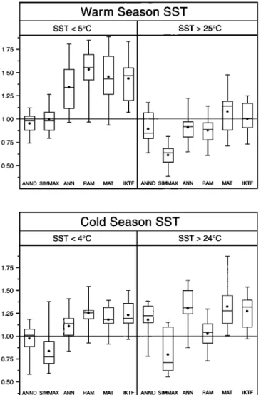
MALMGREN ET AL.' ESTIMATING PAST SEA SURFACE TEMPARATURES 525 1.75 1.50 1.25 1.00 0.75 0.50 Warm Season SST SST < 5øC SST > 25øC • __

ANND SIMMAX ANN RAM MAT IKTF ANND SIMMAX ANN RAM MAT IKTF

1.75

Cold Season SST

SST < 4øC SST > 24øC

..

-- •

ANND SIMMAX ANN RAM MAT IKTF ANND SIMMAX ANN RAM MAT IKTF

1.50

1.25

1.00

0.75

0.50

Figure 5. Summary of the prediction errors (expressed as RMSEP in degrees Celsius) produced by the various techniques for the extreme ends of the SST distribution in the 10 partitions of the training data set. The box-and-whiskers plots depict the minimum, 0.25 percentile, median, 0.75 percentile, and the maximum RMSEP values; circles represent the arithmetic average of the 10 partitions for each technique.

epochs was set to 500 for each configuration. In addition, a criterion was added that instructed the network to stop learning if no improvement in prediction error occurred after 30 consecutive learning epochs.

2.4.6. Artificial neural network with equatorial distance (ANND). With respect to the amount of information used for training, the SIMMAX approach [Pfiaumann et al., 1996] differs from all other methods by including two additional variables to the census counts of the 26 planktonic foraminifer species: the geographical coordinates of the coring sites. To investigate the effect of including such information into databases used for training the BP neural networks, the equatorial distance (directly calculated from latitude) was included as the 27th variable in all partitions. Thereafter, a set of neural networks was trained to predict SSTs from training sets modified in this way. The criteria for network configuration and number of learning epochs were identical to ANN. The average configurations of the trained BP

networks for both the ANN and ANND methods are shown in

Table 2.

3. Results

3.1. Training

The results of the calibration and/or training of the various techniques are shown in Figures 3-5 and Table 3. On the basis of their success in predicting modem SSTs from core top samples, the different techniques can be divided into three distinct groups. For all partitions in both the cold season and warm season SST calibration the IKTF technique produced by far the highest RMSEP values (Figure 3). The magnitude of the difference is

consistently at least 0.18 ø + 0.03øC, and there is very little overlap

between the individual RMSEP values produced by the IKTF and those produced by the other techniques.

ANN, RAM, and MAT seem to yield similar average RMSEP values, though slight differences in the mean values are evident, suggesting that ANN and RAM produce somewhat lower RMSEP than MAT (Figure 3). These differences are, however, negligible

when compared with the >0.18øC contrast in RMSEP between

these techniques and IKTF.

Both SIMMAX and ANND yield the lowest RMSEP values (Figure 3). For the warm season calibrations, ANND yields slightly lower average RMSEP values than SIMMAX, while for the cold season calibrations the values are similar. Interestingly, the average improvement of the prediction error between these techniques and

interpolated set were used for temperature reconstructions. The

parameters we used were o• = 0.2 and 'y = R = 0.2øC.

2.4.5. Artificial neural network (ANN). The general principles and architecture of a back propagation (BP) neural network were described by Malmgren and Nordlund [1996,

1997]. In this application a neurogenetic algorithm was used (NGO v2.5 program) that automatically searches for the configuration of the network that produces the lowest error of prediction. Thus the number of hidden layers (one or two), the number of neurons in each layer (_<32), and the type of transfer function in each neuron (linear, logarithmic, or hyperbolic tangent) were allowed to vary among the different partitions used for training. For each partition the algorithm proceeded through 50 populations of neural networks with 30 generations in each, thus the total number of net configurations examined was 1500 per

partition. Malmgren and Nordlund [1997] noted that a BP network

usually reaches the minimum prediction error after <700 learning epochs. Our experiments showed that, using the learning ability compensation, the minimum prediction error is reached after <500 learning epochs. Therefore the maximum number of learning

Table 3. Mean, Maximum, and Minimum RMSEP Values Produced by the SST Prediction Techniques When Applied to

the 10 Partitions of the Training Database a

RMSEP• øC

Mean Maximum Minimum

Warm Season SST ANND 0.7984 0.8864 0.7125 SIMMAX 0.8636 0.9662 0.7681 ANN 0.9917 1.0703 0.9564 RAM 1.0060 1.0770 0.9590 MAT 1.0506 1.1991 0.9765 IKTF 1.2305 1.2908 1.1933 CoM Season SST ANND 0.9081 0.9930 0.8142 SIMMAX 0.9045 1.0498 0.7589 ANN 1.0794 1.2006 0.9790 RAM 1.0581 1.1450 0.9430 MAT 1.0969 1.2108 0.9352 IKTF 1.2843 1.3832 1.2195

526 MALMGREN ET AL.: ESTIMATING PAST SEA SURFACE TEMPARATURES

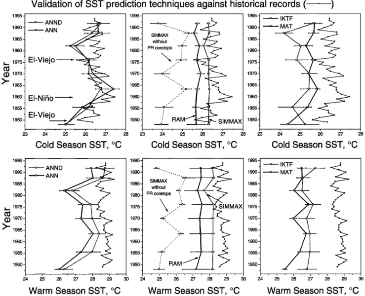
Validation of SST prediction techniques against historical records (

ß )

1995

...

A

NND

•

1990

• ANN

.••

...

1985 •.:•½.•/• SIMMAX

without ,/

"

•/'

19•

.%•.•

•

PR

coretops

.,-Vieio

•96o-

EI-Nifio • _ ••

,,-V.e,o

S.MMAX

Cold

Season

SST,

øC

Id

Season

SST,

øC

Cold

Season

SS•,

øC

1•-

•--•

•o

...

ANND

•

ANN

1980

-•.•.•=,•.•

PR

coretops

',,

: :•-•

•.•

Ax

//

Warm Season SST, øC

Warm Season SST, øC

Warm Season SST, øC

Figure 6. Comparison of reconstructed and measured cold season and warm season SST variation through the time interval recorded in the upper 15 cm of box core PRB-12. Ten different SST estimates were obtained for each sample by using the 10 different partitions of the training data set to generate the estimates. The mean values and 95% confidence intervals (horizontal bars) are shown for each sample. Instrumental measurements (fine lines) were compiled from the COADS data set and from da Silva et aL [1994]. Note that the instrumental record comprises "sea surface" temperatures, while the prediction techniques have been trained to estimate average SST from 0 to 75 m. Therefore the

warm-season SST estimates are expected to be some 0.4øC lower than the instrumental record (see Figure 2).

their counterparts without the geographical information (MAT and

ANN) is approximately equal (ANN minus ANND is 0.24 ø +

0.02øC and 0.17 ø + 0.03øC; MAT minus SIMMAX is 0.19 ø + 0.03øC and 0.19 ø + 0.04øC for warm and cold season SST, respectively; see Figure 3).

All six techniques examined were more successful in predicting warm season SSTs than cold season SSTs (Figure 3). The average

difference between RMSEP values for the two seasons varied

between 0.04 ø + 0.04øC for SIMMAX and 0.11 ø + 0.02øC for

ANND. However, cold season SST prediction seems to be more sensitive to small changes in the training data set, as implied by the larger variability among the RMSEP values from individual partitions (Figure 3).

Whether the various techniques produce consistent prediction error throughout the SST range in the test sets can be addressed by examining the distribution of the residuals (Figure 4) and by calculating RMSEP for both extremes of the SST range (Figure

5). The most prominent feature in the plots of the residuals (i.e., the predicted minus the observed SST values) is the presence of a "tail" at the cold end of the SST range (Figure 4). This feature translates the fact that the estimated SSTs are systematically

warmer than the coolest observed SSTs and are colder than the

immediately adjacent cold SSTs. This phenomenon is caused by the extremely low diversity of polar planktonic foraminifer faunas, which show decreasing change in composition with decreasing SST values [see also Pfiaumann et aL, 1996]. The plot of the residuals in Figure 4 also reveals that all the methods consistently underestimate the warmest SSTs.

The RMSEP values calculated for the extremes of the SST range

(<5øC and >25øC for warm season and <4øC and >24øC for cold

season) reveal several interesting features about the SST predic- tions (Figure 5). In the warm season SST predictions all techniques were more successful in estimating the warm end SSTs and less successful in estimating the cold end SSTs. As expected from the

MALMGREN ET AL.: ESTIMATING PAST SEA SURFACE TEMPARATURES 527

distribution of the residuals in Figure 4, ANND and SIMMAX yielded much lower RMSEP for the cold end SST predictions, most probably as a consequence of the substitution of faunal variation in the cold end samples by the geographical information. In the cold season SST predictions all techniques were either equally successful for both ends of the SST range or, in some cases, were more successful in estimating the cold end SSTs and were less successful in estimating the warm end SSTs.

The performance of some techniques in extremes of the SST range did not conform to the general ranking based on the prediction errors from the entire SST range (Figure 3 and Table 3). Thus, being very successful in predicting SST in both extremes of the SST range, SIMMAX must inevitably produce larger errors in the remaining part of the SST range. The RAM technique produced the highest RMSEP values in the cold end predictions for both seasons and the second lowest RMSEP values for the warm end predictions for both seasons. Consequently, it appears that this technique is more efficient in predicting warmer SSTs. Contrary to the general ranking, in the extreme end SST predictions the IKTF technique produced similar or even lower RMSEP values than ANN and MAT. This implies that IKTF yields a large error of prediction throughout the SST range, while ANN and MAT are more successful in predicting SSTs between the extremes of the SST range.

3.2. Validation

The SST in the Caribbean Sea south of Puerto Rico varied

significantly over the past •50 years (Figure 6). The variation appears largely decoupled between warm season and cold season SSTs. The cold season SST signal manifests larger variability with

SST values between 25.5 ø and 27.5øC. The warm season SST signal

shows less variability with values between 28.2 ø and 29.2øC. The highest warm season SST in the training data set was 28.54øC. This implies that a certain part of the warm season SST variation falls outside of the range represented in the training data set.

With respect to the cold season SST reconstruction the ANN and ANND methods yielded exceptional results, with reconstructed SSTs matching the absolute values and general trends in the instrumental record. Both methods succeeded in reconstructing the most prominent features of the recorded cold season SST series: the unusually cold winters of the E1 Viejo years 1950 and 1973- 1975 and the extremely warm winters of the E1Nifio years 1957- 1958 (Figure 6). Despite the substantial difference in their ability to reconstruct modem SST, because of the addition of the geograph- ical information in ANND, both methods yielded virtually identical cold season SST reconstructions for core PRB-12.

SIMMAX and RAM methods succeeded in reconstructing the

absolute values of the recorded cold season SST. However, both

methods failed to reconstruct the SST variation. This is especially true for SIMMAX, which only produced reasonable SST recon- structions when the two Caribbean core tops were retained in the training database. Because of the close proximity of both core tops to PRB-12 (the PRB-12 core top was artificially set to be 1 km away; retaining the original distance would mean that the recon- structed SST would have been equal to the core top value for all samples [see Pfiaumann et al., 1996]), the reconstructed SST never deviated from the values recorded in these core tops. When these core tops were removed from the training database, the SST reconstruction departed from the record more than the results of all the other techniques (Figure 6). MAT and IKTF failed to reconstruct even the absolute values of the SST variation. The reconstructed SSTs are lower than the recorded values by as much

as 1ø-2øC (Figure 6). The SST variation reconstructed by MAT

seems to conform better to the variation in the instrumental record

than the SST variation reconstructed by IKTF, which does not

seem to follow the record at all.

The warm season SST reconstructions produced by all methods appear to follow the cold season SST reconstructions, offset by

• 28 03 24 22 z 20 z 18 I 2 3 4 5a 5c 5e 6 ß , 0 1{•0 2(•0 3•)0 400

28

o(")

26 '•

• 24

•,.

I• 24

.:•

• 22

20

p 28

<:• 22

<:• 20

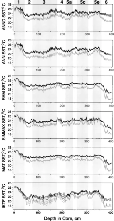
Figure 7. Warm season and cold season SST reconstructions in core V 25-59 derived from the different techniques. Bold lines represent mean values of the 10 estimates produced by each technique; fine lines envelop 95% confidence intervals. The inferred ranges of oxygen isotope stages 1 through 6 follow Mcintyre et al. [1989]. The SST reconstructions for the core presented here depart substantially from those in previous studies [B• et al., 1976; Mcintyre et al., 1989; Waelbroeck et al., 1998]. This fact can be best explained by the choice of a very different training database. While all the previous studies based the reconstructions on global databases including samples from the Pacific and Indian Oceans, our database only includes samples from the Atlantic Ocean.

some 1.5øC toward warmer temperatures. Once the expected 0.4øC

shift due to the difference in the SST def'mition between the

instrumental record and the training data set is taken into account, one could argue that the predictions by ANND, ANN, SIMMAX

528 MALMGREN ET AL.: ESTIMATING PAST SEA SURFACE TEMPARATURES

(with Caribbean core tops), and RAM approach the absolute values of the instrumental record. However, none of the methods fully succeeded in reconstructing the absolute values in the record. This probably reflects the fact that the recorded warm season SST values were above the range of the training database.

3.3. Application to the Fossil Record

In order to assess the potential differences among the SST reconstruction techniques when applied to a large fossil data set, the SST variation during the last • 150 kyr was reconstructed from census counts in tropical Atlantic core V 25-59 (Figure 7). Although the general pattern of variation is similar for all six SST reconstructions, there are significant differences. We will discuss three aspects of the SST reconstructions where these differences are most marked: (1) the pattern and magnitude of the deglacial warming during Termination I (the transition from oxygen isotope stage (OIS) 2 to 1), (2) the SST variability between OIS 2 and OIS 5, and (3) the reconstructed SST values for the glacial OIS 6.

According to both ANN and ANND, Termination I in the tropical Atlantic was relatively abrupt, with the Last Glacial

Maximum ocean being some 4øC (warm season) to 5øC (cold

season) colder than during the Holocene (Figure 7). All three modem analog technique-based methods (RAM, SIMMAX, and MAT) reconstructed Termination I as being more gradual, with a

smaller magnitude of the deglacial warming (•3øC for warm

season SST and •4.5øC for cold season SST). The IKTF SST

reconstruction also appears to suggest that Termination I was gradual, but the magnitude of the deglacial warming was much

larger (•5øC for warm season SST and 7øC for cold season SST).

It should be noted that SST values produced by IKTF for the remaining part of the core (OIS 2-6) are much lower (by almost

2øC) than those produced by the other techniques.

With respect to SST variation during the interval from OIS 2 to OIS 5, the ANN and ANND techniques yielded almost identical

results, suggesting variations of •4øC in both the cold season and

warm season SST (Figure 7). In sharp contrast, the SST variability in this interval reconstructed by RAM, SIMMAX, and MAT is

much weaker (at most 2.5ø-3øC) with most of the variation in cold

season SST. Similar to ANN and ANND, IKTF also reconstructed significant variation between OIS 2 and OIS 5 in both cold season and warm season SST. Interestingly, the 95% confidence intervals for the SST reconstruction in OIS 2-4 are much greater than in any of the other techniques. This suggests that the IKTF SST recon- structions for this interval in core V 25-59 are highly unstable (i.e., a small change in the training database causes large changes in the reconstructions).

The most obvious difference among the SST reconstructions

concerns the SST values for OIS 6, where ANN and ANND

yielded SSTs 2ø-3øC higher than all the remaining techniques

(warm season SST of 22ø-23øC versus 20ø-21øC and cold season SST of 20ø-21øC versus 18 ø- 19øC) and thus were similar to OIS 2 SSTs. This part of the core (below •360 cm) shows signs of calcite dissolution [Bb et al., 1976]. Extremely low SST recon- structions, especially for the cold season, have been produced by all techniques previously used for this core (IKTF [Bb et al., 1976; Mcintyre et al., 1989] and RAM and MAT Waelbroeck et al., 1998]). Thus it appears that the artificial neural networks signifi- cantly differ from all the other SST reconstruction methods by their way of treating no-analog samples.

4. Discussion and Conclusions

4.1. Reconstructing Modern SST

The main conclusions drawn from the RMSEP values for each

technique seem to confirm previously published results. The superiority of all other techniques over IKTF when predicting

modem SSTs has been noted in numerous studies [e.g., Pfiaumann et al., 1996; Malmgren and Nordlund, 1997; Ortiz and Mix, 1997; Waelbroeck et al., 1998]. Here we not only confirmed this pattern but also showed that IKTF SST reconstructions for the validation data set departed most from the instrumental record. Similarly, the SIMMAX technique was considered to yield better predictions of modem SST than MAT [Pfiaumann et al., 1996], which is clearly confirmed by the results of this study (Figure 3 and Table 3). This is not surprising given the fact that the technique enlarges the training database by an additional variable, which is highly correlated with modem SST. An identical improvement in RMSEP is achieved when geographical information is included as an additional variable into the training data set for the BP neural network (ANND). Obviously, the addition of geographical infor- mation imposes severe limits on the use of such techniques: The general assumption that the relationship between variables in the training set and SST remain the same through time can be justified for foraminifer species but certainly not for geographical informa- tion [see Waelbroeck et al., 1998]. Therefore SIMMAX and ANND should not be used for SST reconstructions beyond very recent times (i.e., late Holocene).

Unlike the large differences in RMSEP described above, ANN and RAM seem to yield only a slightly lower RMSEP than MAT (Figure 3 and Table 3). The average difference is very small and not statistically significant. Thus, although ANN and RAM were considered to produce significantly better results than MAT in previous comparisons [Malmgren and Nordlund, 1997; •aelbroeck et al., 1998], our study does not seem to support this conclusion.

4.2. Differences Among SST Predictions

The direct comparison of reconstructed SSTs with an instrumen- tal record indicates that ANN and ANND yielded the best SST estimates (Figure 6). The application of the techniques to the

validation data set also shows that differences in reconstructed

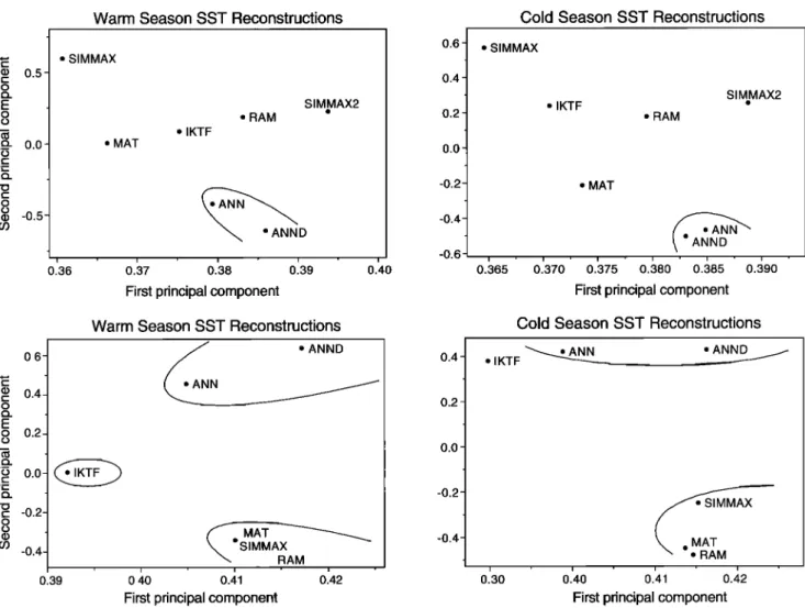
SST do not conform to the performance of the techniques in estimating modem SST (Figure 3 and Table 3). Although ANND and SIMMAX produced the lowest RMSEP for modem samples, the SST reconstructions by ANND were almost identical to those produced by ANN, while SIMMAX estimates resembled much more the SST estimates by RAM. To document this relationship in a quantitative manner, we have performed a Q mode principal component analysis of the SST reconstructions by the different techniques for the validation data set (Figure 8). The analysis demonstrates that the predictions produced by ANN and ANND are very similar to each other while being distinct from those of the other techniques. This conclusion is further supported by the results of SST reconstruction in core V 25-59. A Q mode principal component analysis of SST reconstructions in this core (Figure 8) shows that ANN and ANND produced similar SST estimates, different from those produced by MAT, SIMMAX, and RAM.

The difference in SST estimates between modem analog techni- ques and artificial neural network techniques provides a powerful tool for assessing the reliability of SST estimates in the fossil record. This concept was originally proposed by Hutson [1977]: When techniques based on different approaches yield similar results, the

estimates can be considered more reliable. On the other hand, when

different techniques produce widely diparate results, the estimates are less reliable, either because of the presence of no-analog samples or as a result of secondary modification of the foraminiferal assemblage by calcite dissolution or other processes. Until now, there was no alternative to the modem analog techniques to perform such a comparison because IKTF yields much worse RMSEP.

4.3. Differences Among the Techniques

For a thorough comparison, two additional aspects of the SST reconstruction techniques that have not been mentioned

MALMGREN ET AL.: ESTIMATING PAST SEA SURFACE TEMPARATURES 529

0.5 0.0 -0.5'

Warm Season SST Reconstructions

ß SIMMAX MAT ß IKTF RAM SIMMAX2

0136

0.•37

0.'38

0:39

First principal component

0.6 0.4 0.2 0.0 -0.2 -0.4 -0.6

Cold Season SST Reconstructions

ß SlMMAX ' i

0.'40

0.•365 0.370

0.7s

0.&s0 0.ss

0.90

First principal component

Warm Season SST Reconstructions

0.6 0.4 0.2 0.0 -0.2. -O.4,

•

N

ß

•

ANND

0.•0

0.•1

0142

0.39

0130

First principal component

Cold Season SST Reconstructions

ß IKTF

'•_•.

N

• .MAT

0.'40

0.'41

0.•2

First principal component

Figure 8. Results

of a Q mode

principal

component

analysis

of the SST reconstructions

in (top) core

PRB-12

(Figure

6) and (bottom)

core

V 25-59 (Figure

7) produced

by the six SST prediction

techniques.

Techniques

that

yield similar

SST reconstructions

plot closely

to

each

other

in the diagram.

SIMMAX2 denotes

SIMMAX SST

reconstructions

where

the two Caribbean

core

tops

were

removed

from

the

training data sets.

before must be considered. These are the possibility of retriev-

ing and analyzing separately the information on why the

individual techniques lead to given SST predictions and the

computational efficiency of both the training and the prediction

process.

IKTF has a great advantage over the other methods by providing

clear information on how the SST reconstructions are derived. An

inspection of the principal component scores reveals groups of

species forming "assemblages" typical for various SST regimes.

Similarly, the modem analog techniques also provide valuable

information about how SST estimates are derived. An examination of the "best analog samples" provides information on the modem

environments or parts of the world ocean that are inhabited by

plankton assemblages most similar to those found in a given fossil sample. None of the above can be applied to ANN, for although it is able to "learn" relationships among numbers in a remarkable

Table 4. Summary Comparison of the Six SST Prediction Techniques With Respect to Their Performance in Estimating

SST in the Modem Ocean, in the Validation Data Set, and in the Fossil Data Set

PRB- 12 Validation of

RMSEP Fit to Cold Season SST

Technique Modem Data Values Pattern

ANND best a correct a correct a

ANN good correct a correct a RAM good correct a weak SIMMAX best a correct a none b

MAT

good

wrong

b

weak

IKTF

worst

b

wrongb

wrongb

aResuit is favorable.

bResult is detrimental.

Application to Core V 25-59

Termination I OIS 2-5 Variation OIS 6 Versus OIS 2 SST

abrupt large similar

abrupt large similar

gradual weak much cooler

gradual weak much cooler

gradual none much cooler