HAL Id: hal-03200226
https://hal.archives-ouvertes.fr/hal-03200226
Submitted on 18 Apr 2021
HAL is a multi-disciplinary open access
archive for the deposit and dissemination of
sci-entific research documents, whether they are
pub-lished or not. The documents may come from
teaching and research institutions in France or
abroad, or from public or private research centers.
L’archive ouverte pluridisciplinaire HAL, est
destinée au dépôt et à la diffusion de documents
scientifiques de niveau recherche, publiés ou non,
émanant des établissements d’enseignement et de
recherche français ou étrangers, des laboratoires
publics ou privés.
centennial-to-millennial scale climate variability in an
earth system model of intermediate complexity
T. Friedrich, A. Timmermann, L. Menviel, O. Elison Timm, A. Mouchet,
Didier M. Roche
To cite this version:
T. Friedrich, A. Timmermann, L. Menviel, O. Elison Timm, A. Mouchet, et al.. The mechanism
behind internally generated centennial-to-millennial scale climate variability in an earth system model
of intermediate complexity. Geoscientific Model Development, European Geosciences Union, 2010, 3
(2), pp.377-389. �10.5194/gmd-3-377-2010�. �hal-03200226�
www.geosci-model-dev.net/3/377/2010/ doi:10.5194/gmd-3-377-2010
© Author(s) 2010. CC Attribution 3.0 License.
Geoscientific
Model Development
The mechanism behind internally generated
centennial-to-millennial scale climate variability in an earth system
model of intermediate complexity
T. Friedrich1, A. Timmermann1, L. Menviel1,*, O. Elison Timm1, A. Mouchet2, and D. M. Roche3
1IPRC, University of Hawaii, 2525 Correa Road, Honolulu, HI 96822, USA
2D´epartement Astrophysique, G´eophysique et Oc´eanographie, Universit´e de Li`ege, Li`ege, Belgium
3Section Climate Change and Landscape Dynamics, Department of Earth Sciences, Vrije Universiteit Amsterdam,
De Boelelaan 1085, 1081 HV Amsterdam, Netherlands
*now at: Climate and Environmental Physics, Physics Institute, University of Bern, Bern, Switzerland
Received: 27 January 2010 – Published in Geosci. Model Dev. Discuss.: 25 February 2010 Revised: 13 July 2010 – Accepted: 22 July 2010 – Published: 25 August 2010
Abstract. The mechanism triggering centennial-to-millennial-scale variability of the Atlantic Meridional Over-turning Circulation (AMOC) in the earth system model of intermediate complexity LOVECLIM is investigated. It is found that for several climate boundary conditions such as low obliquity values (∼22.1◦) or LGM-albedo, internally generated centennial-to-millennial-scale variability occurs in the North Atlantic region. Stochastic excitations of the density-driven overturning circulation in the Nordic Seas can create regional sea-ice anomalies and a subsequent reorgani-zation of the atmospheric circulation. The resulting remote atmospheric anomalies over the Hudson Bay can release freshwater pulses into the Labrador Sea and significantly in-crease snow fall in this region leading to a subsequent re-duction of convective activity. The millennial-scale AMOC oscillations disappear if LGM bathymetry (with closed Hud-son Bay) is prescribed or if freshwater pulses are suppressed artificially. Furthermore, our study documents the process of the AMOC recovery as well as the global marine and terres-trial carbon cycle response to centennial-to-millennial-scale AMOC variability.
1 Introduction
Oxygen isotope records from Greenland (Johnsen et al., 1992; Dansgaard, 1993; GRIP Project Members, 1993; NGRIP Project Members, 2004) bear witness to the ex-istence of abrupt climate reorganizations in the Northern
Correspondence to: T. Friedrich
(tobiasf@hawaii.edu)
Hemisphere. Dansgaard-Oeschger (DO) events (Dansgaard et al., 1982; Oeschger et al., 1984), i.e. rapid transitions from stadial to interstadial conditions, are prominent features of the last glacial period. The associated temperature response referred to as the bipolar seesaw pattern (Stocker, 1998) has prompted researchers to hypothesize that their dynamics is tightly coupled to the Atlantic Meridional Overturning Cir-culation (AMOC) (Ganopolski and Rahmstorf, 2001; Alley et al., 2001; Timmermann et al., 2003). In simplified and intermediate complexity models (Stommel, 1961; Broecker et al., 1990; Ganopolski and Rahmstorf, 2001) the AMOC is known to be a nonlinear system with multiple equilibrium solutions and thresholds for transitions between different modes of operation. Stochastic and periodic excitation of such a bistable system can generate dynamical behaviour that resembles the observed DO events (Alley et al., 2001).
In fact, the observed DO events bear some similarity to the so-called ocean relaxation oscillations. Their mecha-nism involves a long “recharging” timescale, often associ-ated with advective or diffusive processes and a rapid “flush-ing” process, such as oceanic convection. Internally gener-ated centennial to millennial-scale relaxation oscillations of the AMOC have been simulated in ocean and climate models of varying complexity (Winton, 1993; Winton and Sarachik, 1993; Paul and Schulz, 2002; Timmermann and Goosse, 2004; Rial and Yang, 2007; Schulz et al., 2007; Jongma et al., 2007; Rial and Saha, 2008) and have often been ex-plained in terms of the deep-decoupling oscillation concept (Winton, 1993). The deep-decoupling phase of such an oscil-lation describes a state with little North Atlantic deep-water formation (due to reduced surface densities). Under such conditions subsurface advective or diffusive heating can lead
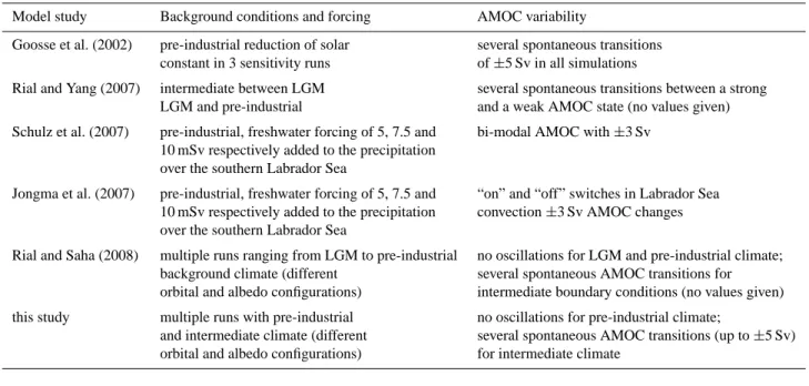
Table 1. Summary of modelling studies that observed low-frequency AMOC oscillations in the ECBilt-CLIO climate model.
Model study Background conditions and forcing AMOC variability
Goosse et al. (2002) pre-industrial reduction of solar several spontaneous transitions constant in 3 sensitivity runs of ±5 Sv in all simulations
Rial and Yang (2007) intermediate between LGM several spontaneous transitions between a strong LGM and pre-industrial and a weak AMOC state (no values given) Schulz et al. (2007) pre-industrial, freshwater forcing of 5, 7.5 and bi-modal AMOC with ±3 Sv
10 mSv respectively added to the precipitation over the southern Labrador Sea
Jongma et al. (2007) pre-industrial, freshwater forcing of 5, 7.5 and “on” and “off” switches in Labrador Sea 10 mSv respectively added to the precipitation convection ±3 Sv AMOC changes over the southern Labrador Sea
Rial and Saha (2008) multiple runs ranging from LGM to pre-industrial no oscillations for LGM and pre-industrial climate; background climate (different several spontaneous AMOC transitions for orbital and albedo configurations) intermediate boundary conditions (no values given) this study multiple runs with pre-industrial no oscillations for pre-industrial climate;
and intermediate climate (different several spontaneous AMOC transitions (up to ±5 Sv) orbital and albedo configurations) for intermediate climate
to a de-stabilization of the water column in the convective areas of the North Atlantic and eventually a convective flush that enhances North Atlantic Deep Water Formation and the meridional overturning circulation. Such flushes are associ-ated with increased poleward heat transport that may provide a self-limiting negative feedback to the AMOC.
Several modelling studies aimed at analysing the mecha-nism triggering DO events using the ECBilt-CLIO climate model (Table 1). The findings of Schulz et al. (2007) and Jongma et al. (2007) indicate that small freshwater perturba-tions in the Labrador Sea can lead to a bi-stable behaviour of the AMOC under Holocene climate conditions. Jongma et al. (2007) conclude that their results give further sup-port hypothesis on the existence of a multi-centennial scale amplifying mechanism that operates under Holocene condi-tions.
Using the same earth system model the studies by Rial and Yang (2007); Rial and Saha (2008) have claimed that Green-land ice-core data can be interpreted in terms of a frequency modulated relaxation oscillation. According to their hypoth-esis internally generated deep-decoupling oscillations in the North Atlantic become frequency modulated by orbitally-induced changes of the solar radiation.
A multi-millennia simulation by Goosse et al. (2002) ex-hibited abrupt climate events lasting for several centuries caused by transitions in the AMOC. Their sensitivity experi-ments showed that a reduction in solar irradiance can trigger the observed transitions.
Inspired by these findings, we set forth to further elucidate the physical mechanisms responsible for the generation of centennial-millennial-scale climate variability in the
ECBilt-CLIO climate model. In set of experiments using different climate background conditions we can qualitatively repro-duce the low-frequency AMOC oscillations described in the publications above. We will show that the underlying mech-anism in the model must be fundamentally different from the one that caused DO events during the last glacial period. Ir-respective of the triggering mechanism we analyse the global impact of the AMOC weakening and the mechanism that leads to its resumption.
This paper is organized as follows: after a brief description of the model and the experiments in the subsequent two sec-tions (2 and 3), we describe the main results from a suite of climate sensitivity experiments in Sect. 4. In Sect. 5 we dis-cuss and summarize the main implications of our findings.
2 Model configuration
We conducted a series of climate sensitivity experiments using the atmosphere-ocean-sea ice-carbon cycle model LOVECLIM (Driesschaert, 2005). LOVECLIM is based on the ECBilt-CLIO EMIC extended by vegetation and marine carbon cycle components.
Its sea ice-ocean component (CLIO) (Goosse et al., 1999) consists of a primitive equation level model with 3◦×3◦ re-solution on a partly rotated grid in the North Atlantic. CLIO uses a free surface and is coupled to a thermodynamic-dynamic sea ice model. In the vertical there are 20 unevenly spaced levels with a thickness ranging from 10 m near the surface to ∼700 m below 3000 m. Mixing along isopycnals, vertical mixing as well as the effect of mesoscale eddies
on transports and mixing and downsloping currents at the bottom of continental shelfs are parametrized. The Bering Strait is closed in our simulations which inhibits freshwater transport from the Pacific into the Arctic.
The atmosphere model (ECBilt) is a spectral T21, based on quasigeostrophic equations with 3 vertical levels and a horizontal resolution of about 5.625◦×5.625◦. Ageostrophic forcing terms are estimated from the vertical motion field and added to the prognostic vorticity equation and thermody-namic equation. Diabatic heating due to radiative fluxes, the release of latent heat and the exchange of sensible heat with the surface are parametrized. The seasonally and spatially varying cloud cover climatology is prescribed in ECBilt.
The ocean, atmosphere and sea ice component of the ECBilt-CLIO model are coupled by exchange of momen-tum, heat and freshwater fluxes. The hydrological cycle over land is closed by a bucket model for soil moisture and sim-ple river runoff scheme. Due to the weakness of the tropical trade winds simulated by the model, the moisture transport from the Atlantic to the Pacific is too weak. To generate an Atlantic salty enough for an AMOC, a small correction for freshwater flux is prescribed redirecting snow- and rainfall over the Atlantic to the North Pacific.
The terrestrial vegetation module of LOVECLIM, VE-CODE is described by Brovkin et al. (1997). On the ba-sis of annual mean values of several climatic variables, the VECODE model computes the evolution of the vegetation cover described as a fractional distribution of desert, tree, and grass in each land grid cell once a year. Within the LOVE-CLIM version used here, simulated vegetation changes affect only the land surface albedo, and have no influence on other processes such as evapotranspiration or surface roughness.
LOCH is a 3-D global model of the oceanic carbon cycle with prognostic equations for dissolved inorganic carbon, to-tal alkalinity, phosphate , organic products, oxygen and sil-icates (Mouchet and Francois, 1996). LOCH is coupled to CLIO, using the same time step. Biogeochemical tracers in LOCH are advected with the CLIO circulation field and are subject to horizontal and vertical mixing. The phytoplankton growth depends on the availability of nutrients (phosphate) and light, with a weak temperature dependence. A grazing process together with natural mortality limit the primary pro-duction and provide the source term for the organic matter sinking to depth. The atmospheric CO2content is predicted
for each ocean time step from the air-sea CO2fluxes
calcu-lated by LOCH as well as from the air-terrestrial biomass CO2fluxes provided by VECODE.
A more detailed description of the LOVECLIM model together with an evaluation of its performance under present-day and LGM climate can be found in Menviel et al. (2008).
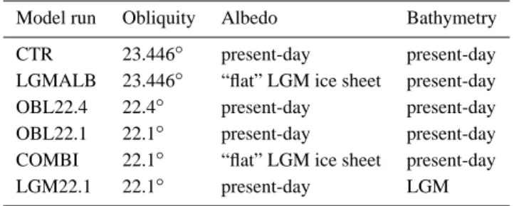
Table 2. Acronym, obliquity, albedo and bathymetry for different
model runs. For all runs eccentricity, precession, sea level, land topography and atmospheric CO2concentration were kept at
pre-industrial values.
Model run Obliquity Albedo Bathymetry CTR 23.446◦ present-day present-day LGMALB 23.446◦ “flat” LGM ice sheet present-day OBL22.4 22.4◦ present-day present-day OBL22.1 22.1◦ present-day present-day COMBI 22.1◦ “flat” LGM ice sheet present-day LGM22.1 22.1◦ present-day LGM
3 Experiments
A set of experiments was conducted to study the parameters settings under which the model exhibits internally-generated low-frequency variability of the AMOC as well as the trig-gering mechanism (Table 2). A pre-industrial baseline sim-ulation was obtained with LOVECLIM by first prescribing present-day orbital parameters, bathymetry, land albedo and topography and by forcing the model with an atmospheric CO2concentration of 287 ppmv for 500 years. Thereafter by
activating the coupling between the carbon cycle and the cli-mate components, the atmospheric CO2 concentrations are
allowed to vary freely for another 1700 years. The mean climate of the baseline run was described in Menviel et al. (2008). A new control run (CTR, in Table 2) was integrated from this equilibrium for 8000 years. Subsequently, several model runs were conducted for at least 5000 years using dif-ferent values for obliquity and northern-hemispheric albedo respectively while keeping pre-industrial values for all other boundary conditions (see Table 2). In addition, a 2000 year-long sensitivity run was performed with LOVECLIM using LGM-bathymetry values (Roche et al., 2007) and an obliq-uity value of 22.1◦.
In the present study the model is exclusively forced by dif-ferent obliquity and albedo values. No use has been made of additional constant (Schulz et al., 2007) or time-varying (Ganopolski and Rahmstorf, 2001) freshwater perturbations.
4 Results
4.1 AMOC response to different background climate
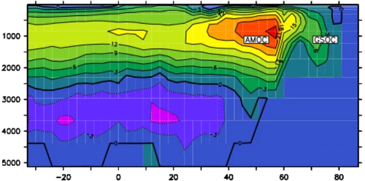
The climatological formation sites of North Atlantic Deep Water in our model are located in the eastern Greenland Iceland Norway (GIN) Sea, Labrador Sea and Irminger Sea. The meridional streamfunction of the CTR run that characterizes the Atlantic meridional overturning circulation (Fig. 1) exhibits the two main deepwater formation branches: one north and one south of the Greenland-Scotland Ridge.
Fig. 1. Mean Atlantic Meridional Overturning Circulation for the
control simulation in Sv. The two cells that are referred to in the text – GIN Sea overturning circulation (GSOC) and maximum of Atlantic overturning circulation (AMOC) – are indicated by the la-bels.
In the following we will refer to GIN Sea overturning cir-culation as “GSOC” and to the maximum of the Atlantic meridional overturning circulation (including the GIN Sea) simply as “AMOC”. We define the GSOC index as the max-imum value of the meridional stream function north of the Greenland-Scotland Ridge, whereas the AMOC index refers to the overall maximum of the streamfunction in the North Atlantic.
Figure 2 compares the simulated variations in the GSOC and the AMOC for the control run (CTR) and the four runs under different climate boundary conditions (LGMALB, OBL22.4, OBL22.1, COMBI). The overturning indices in the CTR run under present-day climate conditions do not exhibit any significant low-frequency variability (Fig. 2a, f). The LGMALB run is characterized by an increased GSOC variability (Fig. 2b) and an abrupt weakening “event” in both indices which lasts for about 200 years similar to results of Goosse et al. (2002). Lowering obliquity from 23.444 to 22.4 has a similar but somewhat stronger effect on the low-frequency variability (Fig. 2c, h). GSOC varies by about
±2.5 Sv and these variations are accompanied by numerous abrupt transitions between a strong AMOC state (∼26 Sv) and an intermediate state (∼19 Sv). The timescale of this variability ranges from 1000–1500 years. Further reduction of the obliquity to 22.1◦(Fig. 2d, i) leads to a shift of the pause-pulse ratio: the AMOC is now preferentially operat-ing in the intermediate regime (∼19 Sv), rather than in the strong AMOC state. Similar changes of the pause-pulse ratio of millennial-scale AMOC variability can be induced by ex-ternal freshwater forcing, as described in the idealized box-modelling study of Schulz et al. (2002) and the LOVECLIM modelling study of Schulz et al. (2007) and Jongma et al. (2007). For a combination of low obliquity and a LGM-albedo (COMBI run) abrupt transitions appear to be less fre-quent and the intermediate regime is characterized by higher AMOC values (∼23 Sv).
4.2 Mechanism of centennial-to-millennial-scale AMOC variability
To elucidate the physical mechanisms responsible for the generation of centennial-to-millennial-scale GSOC and AMOC variability, we focus on only one event in the OBL22.4 run (model years 2450–3050). Further statistical analysis (not shown) revealed that the same mechanism oper-ates in the other experiments and for other individual events. Figure 3b–g documents crucial stages during an AMOC cycle in the OBL22.4 experiment as well as the associated states of the two overturning cells (Fig. 3a). In our sim-ulation an event is initiated by a random reduction of the GSOC. This reduction leads to a decrease of meridional heat transport into the GIN Sea and an associated decline in SST in the sinking region of ∼2–5 K (not shown). The drop in SST causes an increase in sea ice coverage in the consid-ered region (not shown). The position of the sea ice (defined here as the position of the 0.1 m sea ice thickness contour) shifts southward by several degrees latitude, now covering the major part of the sinking region. Sea ice insulates the ocean surface from heat loss which leads to a further reduc-tion of the strength of the overturning (Fig. 3b). As a con-sequence of the sea-ice expansion, surface air temperature (SAT) decreases in the Nordic Seas by up to 20 K (Fig. 3c, shaded). The resulting geopotential height anomaly over the eastern North Atlantic exhibits a baroclinic structure in the vertical similar to the response to negative SST anomalies in Deser et al. (2004). A surface boundary layer high pres-sure anomaly develops over the GIN Sea that is accompa-nied by low pressure anomalies over southern Greenland and the Hudson Bay (Fig. 3c, contours). As we shall see later the resulting wind stress anomalies over the Hudson Bay are crucial for the reduction of Labrador Sea convection and eventually the weakening of the AMOC. Due to the model representation of river runoff, sea surface salinity (SSS) in the Hudson Bay is about 1.4 psu lower (∼33.60 psu) than in the adjacent Labrador Sea (∼34.98 psu) – in accordance with the Levitus Climatology (Levitus, 1994). Under clima-tological conditions the zonal salinity gradient between Hud-son Bay and Labrador Sea is maintained by north-westerly winds. As a result of the altered near surface pressure pat-tern (Fig. 3c, contours), the meridional wind stress compo-nent near Hudson Strait is strongly reduced which results in a flush of fresher water from the Hudson Bay into the Labrador Sea (Figs. 3c, d and 4a). Moreover, the anomalous low pres-sure near Hudson Bay leads to a significant increase in snow fall further freshening surface waters (Fig. 4c). The resulting drop of SSS in the Labrador Sea (Fig. 3d, contours, Fig. 4c) leads to a major reduction of Labrador Sea convection and a subsequent decrease of the North Atlantic overturning cir-culation strength by about 8 Sv (Fig. 3a–phase d). A part of this fresh surface water is advected from the Labrador Sea into the GIN Sea, thereby maintaining the halocline in the GIN Sea. In OBL22.4 this state of reduced overturning lasts
Fig. 2. GIN Sea overturning circulation (GSOC) (a–e) and maximum of Atlantic overturning circulation (AMOC) (f–j) in Sv for indicated
model simulations. Please refer to Table 2 for an explanation of the simulations. A low pass filter of 50 years was applied for green lines.
for about 300 years. Anomalies in the annual mean convec-tive layer depth (CLD) attain values of up to −200 m in the Labrador Sea and up to −400 m in the GIN Sea1. The at-mospheric response pattern to the GIN Sea near-surface tem-perature anomalies is persistent throughout the entire period of AMOC weakening (Fig. 3e). The recovery phase of the AMOC (Fig. 3f, g) is associated with subsurface warming
1In wintertime these anomalies are much larger.
of the GIN Sea (Fig. 3f). Subsurface temperature anoma-lies in this region reach values of up to 4 K. Compared to the unperturbed variance of subsurface temperature variations of 0.26 K, a 4 K anomaly during the recovery phase represents an unprecedented warming of the subsurface and deep-water layers – a phenomenon known as deep decoupling. Even though GSOC is strongly reduced in phases e and f (see Fig. 3a), warm and salty water from the North Atlantic Drift
Fig. 3. (a) Anomalies of AMOC (black) and GSOC (blue) in Sv for the OBL22.4 run for the timeframe 2450–3050 (see also Fig. 2c,h).
Dashed vertical lines denote averaging intervals for panels b-g of this figure. (b) Anomalies in convective layer depth (CLD) in m (shaded) and surface heat flux (HFLX) in W/m2(contours). A positive HFLX anomaly is associated with a lower-than-normal heat loss of the surface ocean to the atmosphere. The red line indicates the mean GIN Sea sinking region in the model. (c) Anomalies of surface air temperature (SAT) in K (shaded), 800 mbar geopotential height in m2/s2(contours) and surface wind stress in N/m2(arrows). (d) Anomalies of sea surface height in m (shaded) and sea surface salinity in psu (contours). (e) Anomalies in CLD in m (shaded), 800 mbar geopotential height in m2/s2(contours) and surface wind stress in N/m2(arrows). (f) Anomalies of oceanic temperature in K averaged over 200–5500 m. (g) SAT anomalies in K (shaded) and CLD anomalies in m (contours). All anomalies in panels b-g are calculated against a strong AMOC state (years: 2400–2450) and averaged over the interval indicated by the respective letter in panel a.
is still advected into the Nordic Seas and the Arctic at depths of 500–1500 m. Due to the lack of deep ocean convection, the inflowing warm and salty North Atlantic waters are not mixed with colder surface waters any more. The subsurface temperatures and salinities in the GIN Sea become decou-pled from the surface processes. Decomposing the impact of deep decoupling on the vertical density gradient reveals op-posing effects of thermal and haline density components. In the absence of mixing with fresher surface water a salinity anomaly of 0.2–0.4 psu forms in depths >800 m. In con-junction with surface salinities being lower by about 2 psu
this tends to stabilize the water column. But in the course of an AMOC weakening event the anomalies in vertical temper-ature gradient outbalance the ones in salinity and the water column becomes unstable. The increase of subsurface heat content eventually reduces the vertical density gradient to a point when surface convection is re-initiated (Fig. 3g). Pre-viously stored subsurface heat is vented to the surface. Sea-ice coverage reduces and surface air temperature increases by up to 10 K. Associated atmospheric circulation changes generate surface wind anomalies near Hudson Bay, a reduc-tion of snow fall in that area and a re-establishment of the
Fig. 4. Timeseries of variables for OBL22.4 run: (a) meridional wind stress at Hudson Strait (80◦W:70◦W, 60◦N:70◦N) (red) in N/m2 and Hudson Bay (100◦W:75◦W, 52◦N:70◦N) sea surface height in m (blue) for OBL22.4 run. (b) AMOC in Sv for OBL22.4 run for comparison. (c) SSS in psu (red) and snow fall in cm/a (blue) averaged over Hudson Bay and Labrador Sea (100◦W:45◦W, 50◦N:70◦N) for OBL22.4 run in Sv. A running mean of 25 years was applied for all timeseries.
original zonal salinity gradient between the Hudson Bay and the Labrador Sea. These processes initiate the recovery of the AMOC. As stated in the preceding analysis, meridional wind stress at the Hudson Strait as well as snow fall over the Hudson Bay and the Labrador Sea form the key elements for triggering an overturning weakening in the Labrador Sea. Figure 4 shows a timeseries of these variables for the entire OBL22.4 model simulation. It becomes apparent that for all AMOC reductions observed in our simulation a meridional wind stress at the Hudson Strait and an increase in snow fall in this region is in phase with a decreasing AMOC demon-strating that the mechanism described above applies for all individual AMOC events.
A more detailed analysis of the stochastic excitations of the GSOC (not shown) revealed the link between background climate and role of sea ice in amplifying random negative GSOC anomalies. A randomly occurring negative GSOC anomaly reduces poleward heat transport into the sinking re-gions. The resulting local increase of sea ice depends on the background climate. With lower obliquity values or a higher albedo respectively and hence colder summers there
is a greater chance for the sea-ice anomaly to persist into the winter season. This leads to a reduction of air-sea fluxes and eventually an amplification of the negative GSOC anomaly. If these anomalies persist, the resulting atmospheric response (Fig. 3c) can trigger the mechanism described above.
4.3 Sensitivity experiments
To further elucidate what physical processes are responsi-ble for the generation of simulated millennial-scale AMOC variability a series of sensitivity experiments was conducted. A key component of the proposed mechanism (Sect. 4.2) is the large-scale atmospheric response to GIN Sea tempera-ture anomalies, which plays a fundamental role in flushing Hudson Bay freshwater anomalies into the Labrador Sea and hence in weakening the AMOC.
Here, we will address the question whether the simulated atmospheric anomaly pattern (Fig. 3c) is a consequence of the initial GSOC weakening and how it interacts with the latter.
Fig. 5. (a) GIN Sea SAT anomaly (averaged over 15◦W to 30◦E and 65◦N to 80◦N) with respect to the model years 1 to 50 of the sensitivity experiment. The red lines separate the three stages of the experiment. (b) Anomalies in SAT in K (shaded), 800 mbar geopotential height in m2/s2 (contours) and wind stress (arrows) with respect to the model years 1 to 50 of the sensitivity experiment. The red rectangular indicates the region where the SST perturbation is applied to the GIN Sea atmosphere. Please refer to Sect. 4.3 for details.
We repeated the OBL22.4 run starting from a strong AMOC state. In the first 50 model years a sea surface temper-ature (SST) climatology was generated. Subsequently this climatology was applied for 200 model years everywhere as a lower boundary condition for the atmospheric model, except for the GIN Sea, where simulated temperatures were low-ered artificially by lowering SST (as seen by the atmospheric model) year-round by an additional 3 K (see Fig. 5b).
There-Fig. 6. (a) GSOC for original OBL22.4 run (blue) and (red) a restart
of OBL22.4 run in which a temperature and salinity “climatology” in the Hudson Bay was generated from the years 2401 to 2450 and prescribed for 950 model years. (b) Same as in (a) for AMOC. Please refer to Sect. 4.3 for details.
after, climatological SST forcing was applied for another 200 model years. Figure 5 shows the SAT, 800 mbar geopo-tential height and surface wind stress response to the GIN Sea SST perturbation. Anomalous high pressure forms in the eastern GIN Sea in response to the lower-than-normal SST. Low pressure anomalies develop over Greenland and east of the Hudson Bay, in good qualitative agreement with the di-agnosed atmospheric circulation changes during a weakened GSOC state (Fig. 3c). This experiment supports the notion of a strong atmospheric teleconnection between the GIN Sea and the western North Atlantic that was proposed in Sect. 4.2 to explain the connection between GSOC and AMOC.
In a second sensitivity run we further investigated the role of the Hudson Bay in triggering the observed AMOC os-cillations. The OBL22.4 run was repeated starting from model year 2401 during a strong AMOC state (see Figs. 2c, h and 3a). In the first 50 model years temperature and salin-ity climatology was generated for the Hudson Bay and sub-sequently applied for 950 years. As can be seen in Fig. 6, the initial GSOC reduction still occurs in the perturbed run. However, due to prescribed salinity and temperature in the Hudson Bay a fresh water pulse is suppressed and the tele-connection between GIN sea and Labrador Sea described above cannot be established. Thus the GSOC reduction does not trigger a convection shut-down in the Labrador Sea.
Fig. 7. Hovmoeller diagrams of temperature averaged over GIN Sea in◦C for original OBL22.4 run (a) and (b) a restart of OBL22.4 run in which a subsurface temperature “climatology” in the GIN Sea was generated from the years 2801 to 2850 and prescribed for years 2851 to 3000. Subsequently the model were run another 300 years with prognostic temperatures in the GIN Sea. (c) GSOC for original (black line) and manipulated (blue line) OBL22.4 run in Sv for timeframe 2801–3300. Please refer to Sect. 4.3 for details.
To demonstrate the effects of subsurface ocean warming on the recovery of the GSOC we designed a fully coupled experiment in which subsurface temperatures between 200– 5500 m were climatologically prescribed in the GIN Sea dur-ing a weak GSOC phase. In this sensitivity experiment we repeated the OBL22.4 run for 500 years starting in a weak GSOC/AMOC state (year 2801, see Figure 2c,h). Here, the first 50 model years were used to create a subsurface tem-perature climatology for the GIN Sea. This climatology was then prescribed for the GIN Sea for the subsequent 200 years for water depths between 200–5500 m. The model was in-tegrated for another 300 years with prognostic temperatures everywhere, including the GIN Sea. The resulting GSOC and subsurface temperatures (averaged over the GIN Sea) can be
seen in Fig. 7a,b. Shortly after model year 2900 GSOC in the original OBL22.4 (Fig. 7a and black line in c) experiment recovers abruptly. However, in the sensitivity run (Fig. 7b and blue line in c) prescribed subsurface temperatures im-pede further warming of sub thermocline waters in the GIN Sea. Accordingly stratification is not eroded and GSOC stays in a weak state. After returning to fully prognostic temper-atures in the GIN Sea in model year 3001 GSOC increases by about 0.5 Sv and fully recovers in a thermohaline flush around model year 3100. This sensitivity experiment demon-strated that subsurface warming in the GIN Sea, that is remi-niscent of deep-decoupling dynamics, plays a key role in the recovery of the AMOC.
Fig. 8. SAT difference in K (shaded) and precipitation difference in cm/yr (contours) between a strong and a weak AMOC state for the
OBL22.1 run. A weak (strong) state is defined by an AMOC <21 Sv (>27 Sv). See also Fig. 2i. Note the non-linear color scale for SAT difference.
Fig. 9. Red: SAT over Greenland in◦C for OBL22.1 run. SAT was averaged over 60◦W to 30◦W and 60◦N to 80◦N. Blue: AMOC for OBL22.1 run in Sv. A running mean of 25 years was applied for both timeseries.
4.4 Global impacts of millennial-scale AMOC variability
In our model simulations, the consequences of an abrupt AMOC reduction of about 30% (in the case of the OBL22.4 and OBL22.1 run) can be detected on a global scale. Fig-ure 8 shows the simulated composite differences in SAT and precipitation between a strong (AMOC >27 Sv) and a weak (AMOC <21 Sv) AMOC state for the OBL22.1 experiment. The main response pattern is the so-called bi-polar seesaw (Broecker, 1998) with large-scale warming in the Northern Hemisphere and cooling in the Southern Hemisphere. This pattern is associated with a northward displacement of the Intertropical Convergence Zone for strong overturning in the North Atlantic (Fig. 8). Over Greenland, millennial-scale SAT anomalies attain magnitudes of up to 7 K and are closely linked with ±6 Sv AMOC variations (Fig. 9). Simulated millennial-scale surface air temperature variations as well as their corresponding hydrological effects resemble the spatio-temporal characteristics of the well-known DO oscillations (Dansgaard et al., 1982; Stott et al., 2002; EPICA Commu-nity Members, 2006; Tjallingii et al., 2008). The simulated warming over Antarctica during the weak AMOC state ac-counts for ∼50% of the increase in SAT estimated by EPICA Community Members (2006).
Whereas the simulated rainfall anomalies are relatively small (5–10%) over the equatorial oceans, their relative mag-nitudes over the Sahara and the Sahel are very considerable (∼40%). The precipitation and temperature changes induce variations in terrestrial vegetation. Periods characterized by a weak AMOC are associated with a reduced terrestrial carbon stock (Fig. 10a,b). On the other hand, the relatively cold con-ditions prevailing during weak AMOC periods lead to greater CO2 solubility and an increased storage of carbon in the
ocean. During a weak AMOC state, the decrease in terrestrial vegetation is not entirely balanced by increased CO2
solubil-ity. Hence weak AMOC states are accompanied by an over-all increase of atmospheric CO2 by about 6 ppm. A similar
mechanism for externally forced millennial-scale CO2
vari-ations was already proposed in Menviel et al. (2008). How-ever, it was already noted in Menviel et al. (2008) that the details of the terrestrial and marine carbon cycle response to AMOC variations may strongly depend on the climate back-ground state. Under colder and drier glacial conditions, the terrestrial carbon response might be reduced significantly.
Fig. 10. (a) Atmospheric CO2content (red) in ppm and AMOC (blue) for OBL22.1 run. (b) Carbon reservoir anomalies for the ocean (red)
and the vegetation (green) in GtC and AMOC (blue) for OBL22.1 run in Sv. A running mean of 25 years was applied for all timeseries.
Fig. 11. GSOC (a) and AMOC (b) in Sv for an obliquity of 22.1 but LGM-bathymetry. A low pass filter of 50 years was applied for green
lines.
4.5 Effects of LGM bathymetry
The driving mechanism for centennial-to-millennial-scale AMOC variability in our model heavily relies on the emer-gence of freshwater flushes from the Hudson Bay into the Labrador Sea and the subsequent reduction of Labrador Sea convection. However, during the last glacial period Hud-son Bay was covered by the Laurentide ice sheet. Thus we expect that LGM boundary conditions would prevent the generation of low-frequency AMOC variability in the
LOVECLIM model. To demonstrate this effect we re-peated the OBL22.1 run using an estimate of the LGM-ocean bathymetry (LGM22.1 run, Table 2) (Roche et al., 2007). In addition, the river runoff mask as well as the land-sea frac-tion mask were adjusted to LGM values. Atmospheric topo-graphic forcing was kept at present-day values.
Figure 11 clearly shows that LGM-bathymetry suppresses millennial-scale AMOC variability. Even though the GSOC index exhibits some sawtooth behaviour with multiple, rapid increases of ∼1.5 Sv followed by gradual reductions, no
significant centennial-to-millennial scale variability can be seen for the AMOC. A more detailed analysis (not shown) revealed that the atmospheric response to GSOC reductions is similar to the one shown in Fig. 3c with anomalous high-pressure over the GIN Sea sinking region and lower high-pressure between the southern tip of Greenland and Iceland. How-ever, in the absence of a “freshwater pool” such as the Hud-son Bay this atmospheric teleconnection is not able to trigger changes of Labrador Sea convection and hence suppresses AMOC variability.
5 Conclusions
This paper explored the mechanism responsible for the gen-eration of centennial-to-millennial scale AMOC oscillations in the LOVECLIM climate model. Our findings show that these nonlinear and stochastically excited oscillations dis-appear under glacial boundary conditions (namely glacial bathymetry). Similar to the findings presented by Schulz et al. (2007) we conclude that the mechanism identified for our model solution must be fundamentally different from the one that triggered real Dansgaard-Oeschger events during the last glacial period.
We also conducted several experiments with boundary conditions intermediate between pre-industrial and LGM as described in Rial and Yang (2007) and Rial and Saha (2008). We were able to reproduce their modelling results qualita-tively using flat ice-sheet boundary conditions and different orbital configurations. Hence, we assume that the physical mechanism underlying the millennial-scale DO-like oscil-lation in Rial and Yang (2007) and Rial and Saha (2008) is the same as the one diagnosed in our study. How-ever, our closed Hudson Bay experiments and the sensitiv-ity experiment using prescribed salinsensitiv-ity in the Hudson Bay clearly demonstrate that the mechanism that is powering the simulated centennial-millennial-scale oscillations in ECBilt-CLIO/LOVECLIM has to be distinct from the one that trig-gers Dansgaard-Oeschger oscillations in reality – in contrast to the conclusions of Rial and Yang (2007) and Rial and Saha (2008).
The oscillations identified in ECBilt-CLIO described in Schulz et al. (2007) and Jongma et al. (2007) share several important features with the millennial-scale oscillations in our study. Among them are the atmospheric anomaly pat-tern, the magnitude of the AMOC oscillations and the im-portant role of salinity. However, there appear to be key dif-ferences in the model simulations, such as the lack of a con-vection breakdown in the GIN Sea in Schulz et al. (2007). Furthermore, their advective horizontal recovery mechanism for Labrador Sea convection contrasts our deep-decoupling resumption mechanism for the GIN Sea.
While the oscillatory model solution may depend strongly on regional features, such as the existence or absence of the Hudson Bay, the overall simulated teleconnection
pat-terns bear quite some similarity to those observed for DO events. In accordance with numerous paleo-data, we found that the ±6 Sv variations of the AMOC are accompanied by the bipolar seesaw pattern in surface air temperature and large-scale changes of tropical hydroclimate, with the north-ern tropics drying and the southnorth-ern tropics becoming wet-ter for weak overturning in the North Atlantic. Correspond-ing precipitation changes affect the overall terrestrial carbon stock and hence atmospheric CO2. A +6 Sv (−6 Sv) change
of the AMOC generates atmospheric CO2 anomalies of of
−3 ppm (+3 ppm). Future higher resolution ice-core data from Antarctica might help to confirm whether DO events were in fact accompanied by significant CO2 variations in
the direction predicted here.
Our coupled modelling results lend further support to the concept of deep-decoupling oscillations in 3-D coupled cli-mate models. Identified previously in simplified climate models (Ganopolski and Rahmstorf, 2002; Timmermann et al., 2003) or idealized OGCMs (Winton and Sarachik, 1993), our more realistic model configuration demonstrated the possibility for the emergence of deep-decoupling phases in the GIN Sea. By preventing deep-ocean warming in the GIN Sea we were able to suppress the rapid recovery of the AMOC.
Acknowledgements. T. Friedrich and L. Menviel are supported
by the National Science Foundation under grant number ATM-0712690. A. Timmermann and O. Timm are supported by the Japan Agency for Marine-Earth Science and Technology (JAMSTEC) through its sponsorship of the International Pacific Research Center. D. M. Roche is supported by NWO under the RAPID project ORMEN. We thank Andrey Ganopolski and an anonymous reviewer for their constructive and helpful comments that helped to improve the manuscript. This is IPRC number 710 and SOEST contribution number 7974.
Edited by: M. Kawamiya
References
Aeberhardt, M., Blatter, M., and Stocker, T. F.: Variability on the century timescale and regime changes in a stochastically forced zonally averaged ocean-atmosphere model, Geophys. Res. Lett., 27(9), 1303-1306, doi:10.1029/1999GL011103, 2000.
Alley, R. B., Anandakrishnan, S., and Jung, P.: Stochastic Res-onance in the North Atlantic, Paleoceanography, 16, 190–198, 2001.
Broecker, W. S.: Paleocean circulation during the last deglaciation: A bipolar seesaw?, Paleoceanography, 13, 119–121, 1998. Broecker, W. S., Bond, G., and Klas, M.: A salt oscillator in the
glacial Atlantic? 1. The concept, Paleoceanography, 5, 469–477, 1990.
Brovkin, V., Ganopolski, A., and Svirezhev, Y.: A continuous climate-vegetation classification for use in climate-biosphere studies, Ecol. Model., 101, 251–261, 1997.
Dansgaard, W.: Evidence for general instability of past climate from a 250 kyr ice-core records, Nature, 364, 218–220, 1993.
Dansgaard, W., .Clausen, H., Gundestrup, N., Hammer, C. U., Johnsen, S. F., Kristinsdottir, P. M., and Reeh, N.: A new Green-land deep ice core, Science, 218, 1273–1277, 1982.
Deser, C., Magnusdottir, G., Saravanan, R., and Phillips, A.: The effects of North Atlantic SST and sea-ice anomalies on the winter circulation in CCM3, Part II: Direct and indirect components of the response, J. Climate, 17, 877–889, 2004.
Driesschaert, E.: Climate change over the next millennia using LOVECLIM, a new Earth system model including the polar ice sheets, Ph.D. thesis, Universit´e Catholique de Louvain, Louvain-la-Neuve, Belgium, available at: http://dial.academielouvain.be: 8080/vital/access/services/Download/boreal:5375/PDF 01 (last access: 17 August 2010), 2005.
EPICA Community Members: One-to-one coupling of glacial cli-mate variability in Greenland and Antarctica, Nature, 444, 195– 198, 2006.
Ganopolski, A. and Rahmstorf, S.: Rapid changes of glacial cli-mate simulated in a coupled clicli-mate model, Nature, 409, 153– 158, 2001.
Ganopolski, A. and Rahmstorf, S.: Abrupt glacial climate change due to stochastic resonance, Phys. Rev. Lett., 88, 0385011– 0385014, 2002.
Goosse, H., Deleersnijder, E., Fichefet, T., and England, M.: Sen-sitivity of a global coupled ocean-sea ice model to the parame-terization of vertical mixing, J. Geophys. Res., 104(C6), 13681– 13695, 1999.
Goosse, H., Renssen, H., Selten, F. M., Haarsma, R. J., and Op-steegh, J. D.: Potential causes of abrupt climate events: A numer-ical study with a three-dimensional model, Geophys. Res. Lett., 29(18), 1860, doi:10.1029/2002GL014993, 2002.
GRIP Project Members: Climate instability during the last inter-glacial period recorded in the GRIP ice core, Nature, 364, 203– 207, 1993.
Johnsen, S. J., Clausen, H. B., Dansgaard, W., Gundestrup, K. F. N., Hammer, C. U., Iversen, P., Jouzel, J., Stauffer, B., and stef-fensen, J. P.: Irregular glacial interstadials recorded in a new Greenland ice core, Nature, 359, 311–313, 1992.
Jongma, J. I., Prange, M., Renssen, H., and Schulz, M.: Amplifica-tion of Holocene multicentennial climate forcing by mode tran-sitions in North Atlantic overturning circulation, Geophys. Res. Lett., L15706, 34, doi:10.1029/2007GL030642, 2007.
Levitus, S.: Climatological Atlas of the World Ocean, Tech. rep., NOAA Prof. Paper 13, 1994.
Liu, Z., Otto-Bliesner, B.-L., F. He, E. B., R. Tomas, P. C., Carlson, A., J. Lynch-Stieglitz, W. C., Brook, E., Erickson, D., Jacob, R., Kutzbach, J., and Cheng, J.: Transient Simulation of the Last Deglaciation with a new Mechanism for Bølling-Allerød Warm-ing, Science, 325, 310–314, 2010.
Menviel, L., Timmermann, A., Mouchet, A., and Timm, O.: Meridional reogranization of marine and terrestrial productiv-ity during Heinrich events, Paleoceanography, 23, PA1203, doi:10.1029/2007PA001445, 2008a.
Mouchet, A. and Francois, L. M.: Sensitivity of a global ocean car-bon cycle model to the circulation and the fate of organic matter: Preliminary results, Phys. Chem. Earth, 21, 511–516, 1996. NGRIP Project Members: High-resolution record of Northern
Hemisphere climate extending into the last interglacial period, Nature, 431, 147–151, doi:10.1038/nature02805, 2004.
Oeschger, H., Beer, J., Siegenthaler, U., Stauffer, B., Dansgaard, W., and Langway, C.: Late glacial climate history from ice cores, Climate Processes and Climate Sensitivity, 29, 299–306, 1984. Paul, A. and Schulz, M.: Holocene climate variability on
centennial-to-millennial time scales: 2. Internal feedbacks and external forcings as possible causes, in: Climate development and history of the North Atlantic Realm, edited by: Wefer, G., Berger, W. H., Behre, K.-E., and Jansen, E., Springer-Verlag, Berlin, 55–73, 2002.
Pikovsky, A. S. and Kurths, J.: Coherence resonance in a noise-driven excitable system, Phys.l Rev. Lett., 78, 775-778, doi:10.1103/PhysRevLett.78.775, 1997.
Rial, J. and Saha, R.: Stochastic Resonance, Frequency modula-tion and the Mechanisms of Abrupt Climate Change in the Arc-tic, First International Symposium on Arctic Research, Drastic Change Under Global Warming (ext. abs.), Miraikan, Tokyo, 94– 97, 2008.
Rial, J. A. and Yang, M.: Is the frequency of abrupt climate change modulated by the orbital insolation?, edited by: Hemming, S., Geophysical Monograph Series, Washington, DC, 173, 167–174, 2007.
Roche, D. M., Dokken, T. M., Goosse, H., Renssen, H., and We-ber, S. L.: Climate of the Last Glacial Maximum: sensitivity studies and model-data comparison with the LOVECLIM cou-pled model, Clim. Past, 3, 205–224, doi:10.5194/cp-3-205-2007, 2007.
Schulz, M., Paul, A., and Timmermann, A.: Relaxation oscil-lators in concert: A framework for climate change at millen-nial timescales during the late Pleistocene, Geophys. Res. Lett., 29(24), 2193, doi:10.1029/2002GL016144.
Schulz, M., Prange, M., and Klocker, A.: Low-frequency oscilla-tions of the Atlantic Ocean meridional overturning circulation in a coupled climate model, Clim. Past, 3, 97–107, doi:10.5194/cp-3-97-2007, 2007.
Stocker, T.: The seesaw effect, Science, 282, 61–62, 1998 Stommel, H.: Thermohaline convection with two stable regimes of
flow, Tellus, 13, 224–230, 1961.
Stott, L., Poulsen, C., Lund, S., and Thuell, R.: Super ENSO and Global Climate Oscillations at Millenial Time Scales, Science, 297, 222–226, 2002.
Timmermann, A. and Goosse, H.: Is the wind-stress forcing essen-tial for the meridional overturning circulation?, Geophys. Res. Lett., 31, L04303, doi:10.1029/2003GL018777, 2004.
Timmermann, A., Gildor, H., Schulz, M., and Tziperman, E.: Co-herent resonant millennial-scale climate oscillations triggered by massive meltwater pulses, J. Climate, 16(15), 2569–2585, 2003. Tjallingii, R., Claussen, M., Stuut, J.-B., Fohlmeister, J., Jahn, A., Bickert, T., Lamy, F., and R¨ohl, U.: Coherent high- and low-latitude forcing of the Northwest African humidity, Nat. Geo-science, 289, 670–675 doi:10.1038/ngeo289, 2008.
Winton, M.: Deep decoupling oscillation of the oceanic thermoha-line circulation, in: Ice in the Climate System, edited by: Peltier, W. R., Springer-Verlag, Berlin, 417–432, 1993.
Winton, M. and Sarachik, E. S.: Thermohaline oscillations induced by strong steady salinity forcing of ocean general circulation models, J. Phys. Oceanogr., 23, 1389–1410, 1993.