HAL Id: cea-01802385
https://hal-cea.archives-ouvertes.fr/cea-01802385
Submitted on 23 Mar 2020HAL is a multi-disciplinary open access archive for the deposit and dissemination of sci-entific research documents, whether they are pub-lished or not. The documents may come from teaching and research institutions in France or abroad, or from public or private research centers.
L’archive ouverte pluridisciplinaire HAL, est destinée au dépôt et à la diffusion de documents scientifiques de niveau recherche, publiés ou non, émanant des établissements d’enseignement et de recherche français ou étrangers, des laboratoires publics ou privés.
Non-negative non-redundant tensor decomposition
Olexiy Kyrgyzov, Deniz Erdogmus
To cite this version:
Olexiy Kyrgyzov, Deniz Erdogmus. Non-negative non-redundant tensor decomposition. Frontiers of Mathematics in China, Springer Verlag, 2013, 8 (1), pp.41 - 61. �10.1007/s11464-012-0261-y�. �cea-01802385�
Nonnegative non-redundant tensor decomposition
Olexiy KYRGYZOV1,Deniz ERDOGMUS2
1 Laboratoire d’Outils pour l’Analyse de Donn´ees, LIST, CEA,
Gif-sur-Yvette, F-91911, France, E-mail: [email protected]
2 Cognitive Systems Lab, Department of Electrical and Computer
Engineering, Northeastern University, Boston, MA 02115, USA
Abstract Nonnegative tensor decomposition allows us to analyze data in their ‘native’
form and to present results in the form of the sum of rank-1 tensors that does not nullify any parts of the factors. In this paper, we propose the geometrical structure of a basis vector frame for sum-of-rank-1 type decomposition of real-valued nonnegative tensors. The decomposition we propose reinterprets the orthogonality property of the singular vectors of matrices as a geometric constraint on the rank-1 matrix bases which leads to a geometrically constrained singular vector frame. Relaxing the orthogonality requirement, we developed a set of structured-bases that can be utilized to decompose any tensor into a similar constrained sum-of-rank-1 decomposition. The proposed approach is essentially a reparametrization and gives us an upper bound of the rank for tensors. At first, we describe the general case of tensor decomposition and then extend it to its nonnegative form. At the end of this paper, we show numerical results which conform to the proposed tensor model and utilize it for nonnegative data decomposition.
Keywords matrix, tensor, rank-1 decomposition, basis vector frame
1.
Introduction
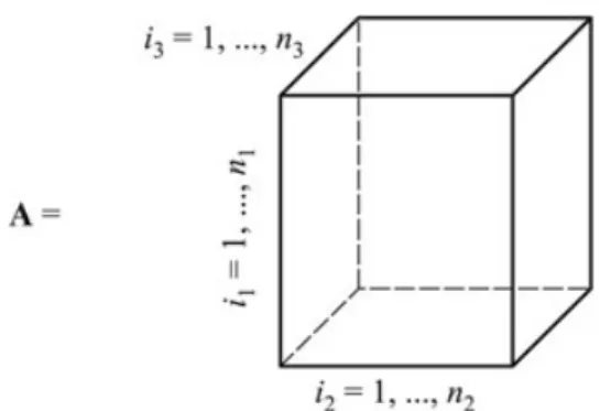
A tensor is a multidimensional array of scalars [10,13]. More precisely, an order-p tensor is an element of the space spanned by the outer product of p vectors, where each vector has its own dimension. The main terms for tensors are the order, dimensions, and the rank which we describe in process of exposition.
The order of a tensor is the number of non-singleton dimensions, also known as ways or modes. There is an example of an order-3 (n1, n2, n3)-dimensional tensor with three different indices in Fig. 1. In general, an order-0 tensor is a scalar, an order-1 tensor is a vector, an order-2 tensor is a matrix, and tensors of order three or higher are higher-order tensors. In this work, we denote vectors by boldface lowercase letters, a, matrices and higher-order tensors (order-3 or higher) by boldface capital letters, A, and scalars by lowercase letters, a.
Fig. 1 An order-3 tensor A ∈ℝ
We propose an alternative decomposition model that utilizes a set of geometrically constrained vectors to generate rank-1 bases. The constraint relaxes the orthogonality assumption in matrix singular value decomposition (SVD) which turns out to be a one-to-one reparametrization of the matrix. The proposition is a generalization of the orthogonal coordinate frame interpretation of the singular vectors of non-symmetric real-valued matrices, which remain as order-2 special cases. The corresponding spacial case of decomposition model for symmetric tensors was proposed and solved for using iterative random search [11].
This paper contributes to the field of tensor analysis and decomposition which appears in signal [14] and image [17] processing, factor analysis [9, 15, 19], speech and telecommunications [10], and bioinformatics. As tensors could emerge from higher-order statistics such as joint moments and cumulants (e.g., consider the symmetric tensor formed by order-p joint moments of an n-dimensional random vector), we believe, tensor decompositions will play an increasingly more important role in statistical signal processing.
The most widely recognized approaches for sum-of-rank-1 tensor decompositions are: (i) canonical decomposition (CANDECOMP) [2] or alternatively parallel factor analysis (PARAFAC) [9]; (ii) the Tucker model [19]. With the CANDECOMP/PARAFAC (CP) model, a tensor can be represented as a sum of rank-1 tensors in a unique fashion without any constrains and the dimensionality of this basis set is the rank:
= ( ) o ( ) o ··· o ( ) (1)
where λ = diag(Λ), u(1) o u(2) o · · · o u(p) denotes the p-way outer-product of the vectors
( ), and upper index (i), i = 1,... , p, denotes the way of product.
Fig. 2 presents a schematic illustration of the CP model, where
( )= ( ), . . . , ( ) , i = 1, . . . , p,
Fig. 2 CP model of an order-3 (n1 , n2 , n3 )-dimensional tensor decomposition
The CP model does not constrain the geometry of the vectors that yield the rank-1 basis tensors; this is in contrast with the assumption of orthogonal vectors in SVD of matrices. While a matrix might be written as a sum of fewer unconstrained left-right vector products than prescribed by SVD, the orthogonality constraint on the geometry of the vectors has been found to be useful in many applications of SVD. As opposed to the CP, Tucker’s proposed decomposition factors tensors as a finite sum assuming orthogonal vectors to generate the rank-1 basis tensors similar to SVD, but the result is not necessarily minimal; in fact, it reparametrizes the tensors with more variables then necessary:
= … "# ,#$….,#% ( )o ( ) o ··· o &
( ) ($)
&
&
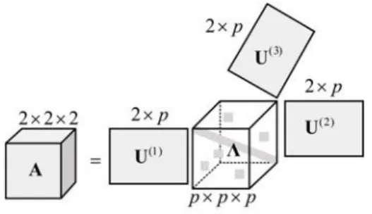
An illustration of Tucker decomposition of an order-3 tensor is presented in Figure 3.
Fig. 3 Tucker model of an order-3 (n1 , n2 , n3)-dimensional tensor decomposition
Nonnegative versions of the CP and Tucker models involve a nonnegative restriction on all their entries. To review comprehensive explanation on the nonnegative tensor decompositions, we refer the reader to the publications of Prof. Andrzej Cichocki from The Riken Brain Science Institute (Japan) [3].
2.
Redundancy and cardinality
There are two differences on the illustrated models: CP model has a diagonal tensor of linear combination coefficients Λ and arbitrary directed vectors in frames U(i), on the
other hand, Tucker model has fully filled tensor of linear combination coefficients Λ
and orthogonal vector frames U(i). When one does
analysis/decomposition/transformation of data, he can say that his method does not loose data when, at least, his method preserves cardinality of data. Cardinality or cardinal number of a set of scalars is the number, c, of free elements (degree of freedom, d.o.f.) in a set, e.g., the cardinal number of any full-rank symmetric two-dimensional matrix equals three. Indeed, any reparametrization (or coordinate transformation) must preserve the cardinality (or the number of dimensions or degrees of freedom).
In Table 1, we present a brief analysis of described models and compare their cardinality with SVD. Let us use a random (2,2)-dimensional matrix A and (2,2,2)-dimensional tensor B. Cardinal numbers of A and B equal 4 and 8, respectively. In the general case, to describe the SVD of A, we need two singular values, r = 2, and, because of orthogonality of vector frames U(i), two rotation angles to define the orientations of orthogonal vector
frames in 2-dimensional space. Therefore, we can see that SVD preserves cardinality of decomposed data. For tensor B, CP models hold r linear combination coefficients and, due to the absence of any restriction on vector frame structure, 3r rotational angles. Suppose that CP model decomposed tensor B with rank r = 1, in this case, CP model does not preserve cardinality, c = 4. For the case of r = 2 cardinality of CP model, c = 8, equals cardinality of tensor B. But the same rank, r = 2, we have for matrix A that is order-2 data. We assume that this case is just a coincidence, because more complicated data must have a higher rank. For rank r = 3 and above cardinality of CP model always higher then cardinality of tensor B.
Tucker model, due to orthogonality of U(i), holds 3 rotation angles for each way of B and r1r2r3 linear coefficients. In any case of values of r1, r2, and r3, Tucker model does not
preserve cardinality of tensor B at all. We need to note that when we apply CP and Tucker models to matrix A, we get the same results as for SVD. Therefore, CP and Tucker models marginally preserve cardinality of data in case when we apply them to matrices and do not do it in the general case.
Table 1 Cardinal properties of existing models of tensor decomposition
matrix SVD CP model Tucker model cardinality of data matrix A[2 × 2] c = 4 tensor B[2 × 2 × 2 c = 8 tensor B[2 × 2 × 2] c = 8 properties of model diagonal Λ orth. U(1) & U(2) diagonal Λ
non-orth. U(1), U(2), & U(3) non-diagonal Λ
orth. U(1), U(2), & U(3) cardinality of model d.o.f. of Λ = 2 d.o.f. of d.o.f. of Λ = r d.o.f. of d.o.f. d.o.f. of of Λ = r1r2r3
U(1) & U(2) = 2 U(1), U(2), & U(3) = 3r U(1), U(2) , & U(3) = 3
c = 4 c = 4r c = 3 + r1r2r3
Below we provide a general model for the case of non-redundant tensor decomposition and then we extend it to nonnegative form.
3.
Decomposition of a symmetric tensor
The decomposition of a symmetric tensor A into a sum of rank-1 tensors [4] utilizes
basis tensors that are p-way outer-products of the same vector (referred to as rank-1 symmetric tensors) [10, 14]:
' = ( (3) where uop denotes the p-way outer-product of the vector u.
Tensor decomposition problem is fundamental to the extension of subspace analysis techniques in signal processing that arise from the study of second order statistics of vector-valued measurements to higher order statistics. Existing examples of such applications include blind source separation. For instance, an exponential multivariate family as a signal model can be factorized using a sum-of-rank-1 tensor decomposition; consider an
n-variate order-p polynomial
*(+) = ' . +( = …
,
' …& . + … +& & ,
where x0 = 1. If the (symmetric) tensor A containing these polynomial coefficients is decomposed into the desired form, then the polynomial can be written as
' . +( = ( -+)
and an exponential density eq(x) can be factorized into a product of univariate
exponentials. Other applications are reviewed by Kolda and Bader [10] and include finding polynomial factorizations [5, 6].
3.1 Order-2 n-dimensional symmetric tensors
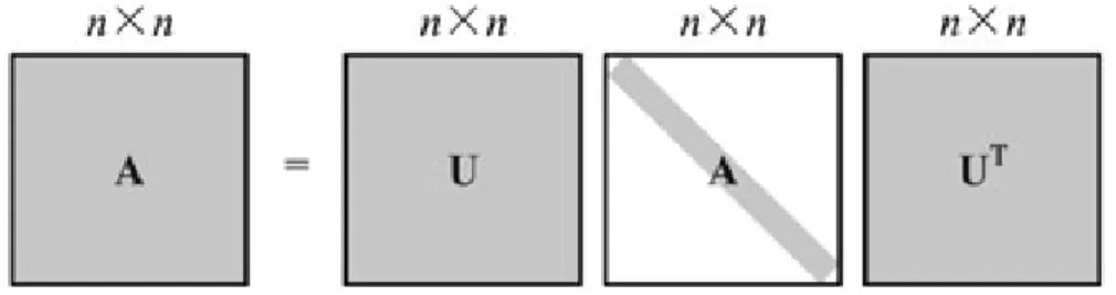
A symmetric n-dimensional order-2 tensor is a symmetric matrix. Eigenvector bases for symmetric matrices are orthogonal, and can always be made into an orthonormal basis. Fig. 4 illustrates the eigendecomposition of a matrix. Thus, a real n-dimensional symmetric matrix can be decomposed as:
' = ( (4)
where
U = [u1,... , un]
Fig. 4 Decomposition of order-2 n-dimensional symmetric tensor
For numerical decomposition of A, we can use, for instance, the Jacobi algorithm [7] that tries to find * = /022 rotation angles {θk , k = 1, . . . , q}, such that we can construct a rotation matrix R(θk) in plane (i, j) (i = 1,... ,n 1, j = i + 1,... , n) with angle θk (with a one-to-one correspondence between the indices k and (i, j) in this Givens angle parametrization). This eigendecomposition solution consists of q rotation angles and n eigenvalues. The number of free elements of a symmetric n-dimensional matrix A,
34 (0, 2) = 0 (0 + 1)2
equals the sum n+q. Consequently, eigendecomposition is simply a reparametrization procedure. Solving for the rotation matrices R(θk), we can get orthonormal eigenvectors given by U :
= 6 7(89) :
9
, ; = ; = < (5)
Due to orthonormality of U, the eigenvalues are uniquely identified by the Frobenius inner-product vector between the target matrix and the basis matrices [10]:
= 〈 ( , '〉
@ = 〈 ( , ( 〉@ = ( - ) (6)
3.2 Order-p 2-dimensional symmetric tensors
Let A be a 2-dimensional order-p symmetric tensor. In a 1-1 reparametrization, the number of linear combination coefficients r, plus the number of parameters that characterize r corresponding vectors s, must be equal to the number of free elements in the tensor1) (i.e., its dimensionality); that is,
r + s = p + 1,
since order-p 2-dimensional symmetric tensors have p + 1 free entries.
1) We do not refer to these coefficients and vectors as eigen until some suitable invariance property is proven.
Incorporating these conditions into the design of the rank-1 sum decomposition on the right-hand side of (3), we obtain that real-symmetric, 2-dimensional order-p tensor A has the
following decomposition: ' = ( , = ⎢ ⎢ ⎢ ⎢ ⎡cos FG + (# − )I% J sin FG + (# − )I% J ⎥ ⎥ ⎥ ⎥ ⎤ (7)
Fig. 5 shows a graphical illustration of the decomposition of order-3 2-dimensional symmetric tensor A.
Fig. 5 Decomposition of order-p (p = 3) 2-dimensional symmetric tensor
In this case, a simple line search for θ in the interval [0, π/p) is sufficient to optimally fit the decomposition to the tensor with zero error. Employing Gram-Schmidt orthogonalization, the linear combination coefficient vector λ is uniquely identified by the product matrix between the basis rank-1 symmetric tensor pairs and the inner-product vector between the target tensor and the basis tensors; i.e., at the optimal decomposition,
λ = diag(Λ) = B−1 c(θ) (8)
Here, the matrix B (invariant with respect to θ, since the pairwise angles between the basis vectors leading to the basis rank-1 symmetric tensors are fixed by the frame) and the vector c are defined elementwise as follows, assuming Frobenius tensor inner product as in (6):
PQ = 〈 ( , Q( 〉@ = 〈 , R〉@ = S - RT , U (8) = 〈 ( , 〉@ (9)
where i, j = 1,... , p. Specifically, note that each entry of B reduces to the following: PQ = cos (W − X)YZ
3.3 Order-p n-dimensional symmetric tensors
The number of free elements of a symmetric n-dimensional order-p tensor is given by 34 (0, Z) = [0 + Z − 1Z \
General structure of vector frames for order-p n-dimensional tensor is presented in the next section, but based on the two special cases examined above, we can conclude that the decomposition of any symmetric tensor can consist of some fixed frame of vectors rotated in n-dimensional space and any angle between pairwise vectors can be constant and depends on order p. As in matrices, we need q rotation angles to decompose any symmetric n-dimensional order-p tensor as a finite sum of rank-1 tensors as in (3). The number of vectors in this decomposition is
] = 3 (0, Z) = [0 + Z − 1Z \ − /022
In Fig. 6, we present a graphical illustration for decomposition of order-3
n-dimensional symmetric tensor A.
Fig. 6 Decomposition of order-p n-dimensional symmetric tensor
To obtain the decomposition numerically, we construct a frame of r initial vectors placed in columns of a matrix F and optimize the q rotation angles θ such that the Frobenius norm of the error tensor is minimized (to zero). In the spirit of block coordinate descent and fixed point algorithms, for a given candidate frame orientation, the linear combination coefficients are always obtained using (9) and (8). The optimization is done iteratively and in a fixed point manner, updating the linear combination coefficients and updating the rotation matrix for the frame of vectors in order to minimize the error tensor Frobenius norm. At each optimization iteration, basis vectors are expressed as follows (all rotations multiply from left):
= ^6 7(89) :
9
4.
Vector frames for symmetric tensors
The assumption that angle between neighbor vectors in n-dimensional space must be equal π/p is not true in general and can be utilized just for order-2 n-dimensional and order-p 2-dimensional tensors. Even for 3-dimensional space, there are exactly 5 convex polyhedra (called Platonic solids) with equal distances between neighbor vectors (or vertices) [18]. For the case of dimensionalities n > 3, there are just three solids with equal distance between neighbor vertexes: cube, octahedron, and simplex.
The vector frame F consists of r vectors fi, i = 1,... , r, defined as its n-dimensional
columns. Based on the cases of vector frames for order-2 n-dimensional and order-p 2-dimensional symmetric tensors, where separation angles between closest vectors are π/2 and π/p, respectively, we can conclude that structure of any vector frame F must maximize minimal distance between vectors (packing procedure) [16]. There is no analytic solution for this task so we propose to solve this problem by iteratively minimizing the squared error (SE):
b2= 〈P − <, P − <〉@ = ] SPR− < RT2 X=1 ] W=1 (11) where, as in (9), PR = S ; RT = Sc; cRT
Vectors fi in frame F can be defined, for instance, in hyperspherical coordinate system
with constant radial values equal 1. Thus, all diagonal entries in B equal 1 and all non-diagonal entries describe distances between vectors or distance between points on hypersphere of unit radius. So minimization of (11) leads to maximization of minimal distances between vectors. Fig. 7 presents results of proposed algorithm for vector frames of different dimensionalities and orders.
We can note that proposed algorithm gives us Platonic solids (convex polyhedra with maximal possible constant distance between nearest vectors) as particular cases of vector frames and empirically, we figured out that for any vector frame planes exist such that frame vectors on those planes separated by π/p radian. This optimization procedure for frame construction gives us r vectors, which yields a full-rank B in (9), and does not engage an elimination procedure as in our previous work that used an overcomplete frame [11].
◦
Fig. 7 (a) Vector frames for 2-dimensional order-3 tensor with 3 unique vectors; (b) 3-dimensional order-2 tensor with 3 unique vectors;
(c) Platonic solid (icosahedron with 6 unique vectors, which does not correspond to any order-p 3-dimensional tensor);
and (d) 3-dimensional order-4 tensor with 12 unique vectors
5.
Decomposition of a non-symmetric tensor
The decomposition of a non-symmetric tensor A into a sum of rank-1 tensors utilizes basis tensors that are p-way outer-products of different vectors (referred to as rank-1 non-symmetric tensors) [10, 14]:
= ( ) o ( ) o ··· o ( ) (12)
where u(1) o u(2) o … o u(p) denotes the p-way outer product and upper index (i), i = 1,.. . , p, denotes the way of product.
5.1 Order-2 (n1, n2)-dimensional non-symmetric tensors
A non-symmetric (n1,n2)-dimensional order-2 tensor is a non-symmetric matrix and we have
to deal with the common case of SVD. Singular vector bases for non-symmetric matrices are always selected orthogonal, and can always be made into an orthonormal basis. Thus, a full-rank (n1, n2)-dimensional non-symmetric matrix can be decomposed
as
where r = min (n1, n2), and
( ) = ( ), . . . , ( ) , ( )= ($), . . . , ($)
are the matrices where columns form orthogonal frames in n1- and n2-dimensional
spaces, respectively, see Figure 8.
Fig. 8 Decomposition of order-2 (n1, n2 )-dimensional non-symmetric tensor
For numerical determination of A, we can use, as in symmetric case, the Jacobi algorithm [7] for each vector frame that tries to find q = q1 + q2 rotation angles
d89( ) , 89( ), e = 1, . . . , * , e = 1, . . . , * f
such that we can construct rotation matrices R(89( )) with angle 89( ) and R(89( )) with angle 89( ), respectively. Due to cross influence of rotation matrices,
* = /02 2 − /0 − 02 2 , * = /02 2 − /0 − 02 2
where /0e2 = 0 if k > n. This singular decomposition solution consists of
q = q1 + q2 rotation angles and r singular values. The number of free elements of a
non-symmetric (n1, n2)-dimensional matrix A equals the product of its dimensionalities so
r = n1 . n2 - q that satisfies definition of the rank in linear algebra, where r = min(n1, n2).
Again, we can see that singular decomposition is simply a reparametrization procedure. Solving for the rotation matrices R(89( )) and R(89( )), we can get the orthonormal singular vectors given by U(1) and U(2) as in (5):
( )= 6 7/8 9g ( )2, S ( )T- ( ) = ( ) S ( )T -= h, W -= 1, 2 (14) :g 9g
Due to orthonormality of U(i), the singular values are uniquely identified by the
Frobenius inner-product vector between the target matrix and the basis matrices [10]: = 〈 ( ) i ( ), '〉@ = 〈 ( ) i ( ), ( ) i ( )〉@ (15)
Described combination of vectors d(1 o 1), (2 o 2),... ,(r o r)f in (13) is not unique [8]. We can construct r! combinations of vectors on the basis of permutation matrices [1], and any of them can be utilized for (n1, n2)-dimensional order-2 non-symmetric tensor
decomposition. Two possible combinations of singular values based on 2-dimensional order-2 permutation matrices are
[ 011 0 \ , [ 0 0 \
Here, the permutation matrix is an order-2 r-dimensional binary-matrix that has exactly one entry of 1 in each row and column and 0’s elsewhere. In case of symmetry,
n-dimensional order-2 tensor vectors can be arranged only in ascending order.
In general, decomposition of an order-2 (n1, n2)-dimensional tensor A, Fig. 8, can consist of
(n1, n1)-dimensional matrix U(1), (n2, n2)-dimensional matrix U(2), and (n1, n2
)-dimensional matrix of singular values Λ. Where singular elements in Λ are located by selecting a permutation matrix. All possible combinations of singular values based in (3,2)-dimensional order-2 matrix Λ are
j 011 0 0 0 k , j 11 0 0 0 0 l k , j 0 0 0 0 k, j 0 00 0 l k , j 00 0 l 0 k , j 00 0 l 0 k
5.2 Order-p 2-dimensional non-symmetric tensors
Let A be a 2-dimensional order-p real non-symmetric tensor. As for the case of symmetric 2-dimensional order-p tensor, we need r linear combination coefficients plus p rotation angles. Since the number of free elements in order-p 2-dimensional non-symmetric tensors equals to product of dimensionalities, the rank of such a tensor is r = 2p- p, where
r ≥ p. We also know that for each way of tensor, we can construct just p vectors.
Incorporating these conditions into the design of the rank-1 sum decomposition on the right-hand side of (12), we obtain that basis frames for this case of tensor A can be expressed as ( )= ⎣ ⎢ ⎢ ⎢ ⎢ ⎢ ⎡cos ^8( ) + /e( ) − 12 Y Z _ sin ^8( ) + /e ( ) − 12 Y Z _⎦⎥⎥ ⎥ ⎥ ⎥ ⎤ , W = 1, … , Z, e( ) ∈ (1, … , Z) (16)
Based on the cases of symmetric 2-dimensional order-p tensors and non- symmetric (n1, n2)-dimensional order-2 tensors examined above, we conclude that the
combinations of vectors d(e( ), e( ), … , e( )f for rank-1 tensors in (12) must be chosen on the basis of a permutation tensor, see Fig. 9. Here, the permutation tensor is an order-p p-dimensional binary-tensor that has exactly one entry of 1 in each way and 0’s elsewhere.
Fig. 9 Decomposition of order-3 (2, 2, 2)-dimensional non-symmetric tensor
The decomposition gives us λ = B−1 c(Θ) , where Θ = [θ(1), θ( 2 ),... , θ(p)].
Here, the matrix B and the vector c are defined elementwise follows, assuming Frobenius tensor inner product as in (9):
PQ = 〈 ( ) i ( ) i … i ( ), Q( ) i Q( ) i … i Q( ) 〉@ (17) p (q) = 〈 ( ) i ( ) i … i ( ), 〉@
where i, j = 1,... , r.
5.3 Order-p (n1, n2, … , np)-dimensional non-symmetric tensors
The number of free elements of a non-symmetric (n1, n2, ..., np)-dimensional order-p
tensor is given by
34 (r, Z) = 0 0 … 0
where r = w0 , 0 , … , 0 x
Based on the two special non-symmetric cases examined above, we conclude that the decomposition of any non-symmetric tensor can consist of some fixed frames of vectors rotated along each way in their dimensionality spaces and any angle between pairwise vectors must be a constant and depends on the order p. As in the case of non-symmetric matrices, we need
* = * + * + ⋯ + * rotation angles. Due to cross influence of rotation matrices,
* = /022 − /0z2 2 , 0z = 0 − 6 0Q {Q{ ,Q|
and therefore, we can decompose any non-symmetric order-p (n1, n2,... , np)-
dimensional tensor as a finite sum of rank-1 tensors as in (12), see Fig. 10. The rank of the tensor in this decomposition is
] = 3 (r, Z) = 34 (r, Z) − *
Fig. 10 Decomposition of order-3 (n1 , n2 , n3 )-dimensional non-symmetric tensor
To obtain the decomposition numerically, we construct p frames each of mr(ni, p) initial
vectors F(i), i = 1, ... , p, and optimize the rotation angles θ(i) such that the Frobenius
norm of the error tensor is minimized (to zero). In the spirit of block coordinate descent and fixed point algorithms, for a given candidate frame orientation, the linear combination coefficients are always obtained using (17) and λ = B−1c(Θ), basis initial
frames are expressed as in Section 4. As in the previous case, we need to choose
r vectors on the basis of an order-p (r1, r2,... , rp)-dimensional permutation tensor, where
] = 3 (0 , Z) , W = 1, . . . , Z
Therefore, at each iteration, basis vectors are expressed as
( )= ^6 7(8 9( )) :
9
_ `( ) (19)
6.
Nonnegative non-redundant tensor decomposition
One of the most awkwardness part of the classical nonnegative CP and Tucker models is the operation of taking nonnegative value, [u]+ = max(0, u) [3]. On each iteration of that
approach, we have to lose some data and try to get new ones without negative entries. It is similar to fitting the model with adjusted random walk. In this section, we present our approach and its analysis for non-redundant tensor decomposition transformed to nonnegative form. The main idea of it is the same as for the described non-redundant one but with one restriction: all linear coefficients λ as well as all entries of the vector frame U must be nonnegative, i.e., stand in positive sector of coordinate system. We do not employ the operator [u]+ and perform optimization procedure as for the general
Let an order-p (n1,... , np)-dimensional nonnegative tensor A be given, i.e.,
ai1,...,ip ≥ 0, which is decomposable as a rank-r tensor with nonnegative values in U
(i), i =
1, . .., p, and λ. With respect to an order-p (r1, ..., rp)-dimensional permutation tensor,
Q, we can write an approximate decomposition of A as
= : g ( ) ( ) o ··· o :g(&) ( ) + ~ (20)
where the tensor E denotes decompose error. The tensor E can contain any possible factors of A with negative inclusions.
As in the case of non-redundant decomposition, we will start to examine an order-p 2-dimensional nonnegative symmetric tensor and then we will extend our approach to the general case of the nonnegative tensor.
Let A be an order-3 2-dimensional nonnegative symmetric tensor. From the non-redundant decomposition of such a tensor, we know that all neighbor vectors are separated by π/3 radian. The range of such a vector frame is from 0 to Y −•
l radians and
solution is a rotation angle θ that lies in the range [0, π/3) radians, see Figure 11 (a).
Fig. 11 Frame vector reorganization for nonnegative non-redundant decomposition
We see that such vector frame, along with its negative part, - F, uniformly covers a unit circle, i.e., all range of ℝ. To restrict our solutions to nonnegative form, ℝ+, we propose to
bound the range of the vector frame, F, in half, i.e., from 0 to •−•
€, see Fig. 11 (b).
Thereby, we have a vector frame that consists of 3 vectors and is invariant to rotation angle π/6, and the rotation angle θ lies in the range [0, π/6) radians. New nonnegative vector frame is the half of the general model frame for an order-6 2-dimensional tensor. Now, we implement nonnegative decomposition of an order-2 3-dimensional tensor A. Involving the idea from the previous example, we need to build the vector frame for an order-4 3-dimensional tensor and utilize the vectors from positive sector only. For the case of an order-4 3-dimensional tensor, the vector frame consists of 12 vectors. The full hypersphere, along with negative form of F, consists of 24 vectors. The 3-dimensional hypersphere has 8 sectors with unique sign of coordinate coefficients. Therefore, in the positive sector, we have 3 required vectors for nonnegative decomposition.
Generalizing these two types of tensors, we can conclude that to get the vector frame, F, for an order-p n-dimensional nonnegative symmetric tensor, we utilize vectors for an order-(2p) n-dimensional common symmetric tensor. Such an approach always gives us the exact number of required vectors, r, in positive sector of n-dimensional space and neighbor vectors are separated by π/(2p) radian.
Till the vector frame stays in positive sector, any projection of A on the vectors ui, i = 1, . .., r, 〈 , ( 〉 is a nonnegative value. To get linear coefficients λ, we also utilize
normalizing matrix B−1, where B = (F FT).p. Some of entries in B−1 are negative, so the final values of λ can be negative.
Actually, for the Monte Carlo experiments (which randomly generate positive entries of the nonnegative tensor) discovered that in the case when the tensor A in not absolutely factorizable in nonnegative form, we have non- zero residual value E in (20).
The general case of nonnegative non-redundant decomposition of an order-p (n1, ..., np)-dimensional tensor is a combination of the expressed nonnegative symmetric
case and the non-symmetric decomposition which is presented above.
Optimization process for such a problem is implemented in the same way as for general case of the tensor. Performing nonnegative decomposition, we involve both vector frame
F and its inversion -F such that any moment we always have the required number of
vectors, r, in positive sector of n-dimensional space.
In Fig. 12, we show the average SE (per tensor entry) for a generated symmetric order-3 2-dimensional tensor. We apply a general vector frame, i.e., angle between neighbor vectors is π/3, and nonnegative one, i.e., angle between neighbor vectors is π/6. For the general vector frame, the decomposition error is periodic with π/3 radians. In the case of the nonnegative vector frame, we cannot decompose tensor at the half of the rotational angle range, π/2, that satisfies to the proposed vector frame squeezing from [0, π) to [0, π/2) radians.
Fig. 12 Symmetric nonnegative order-3 2-dimensional tensor decomposition SE versus rotational angle in range [0, π):
(a) by a frame for general decomposition; (b) by a frame for nonnegative decomposition
7.
Numerical experiments
Bellow, we present evaluation of the proposed tensor model and show numerically that the upper bound of the tensor rank satisfies the defined non- redundant case. We apply nonnegative form and show how it can be used for image segmentations. Matlab code can be downloaded from website [12].
Figure 13 shows how decomposition results for non-symmetric order-3 different-dimensional tensors depend on rank for best rank-r CP1) ‘ ’, incremental recursive rank-1 CP1) ‘+’, Tucker2) ‘o’, and proposed ‘*’ models. When proposed model uses frames of bases with the correct number of vectors, the decomposition error drops to almost zero (with numerical error remaining). Here, on the basis of our definition of the tensor rank, for the data in Fig. 13, we have in case (a), the rank is equal to 5, (b) -14, (c) -18, (d) -46, and decomposition errors are zero. Proposed approach gives us the upper bound of CP-rank for tensors.
rank rank
Fig. 13 Non-symmetric tensor decomposition SE and corresponding tensor rank for rank-r CP ‘ ’, incremental rank-1 CP ‘+’, Tucker ‘◦’, and proposed ‘∗’ models.
(a) (2,2,2)-, (b) (2,3,4)-, (c) (3,3,3)-, (d) (4,4,4)-dimensional tensor
Figure 14 shows how decomposition results for the same non-symmetric order-3 different-dimensional tensors from Fig. 13 depend on cardinality for best rank-r CP ‘Z’, incremental recursive rank-1 CP ‘+’, Tucker ‘o’, and proposed ‘*’ models. Evaluation of the tensor cardinality was performed in the estimated ranks of the tensors. The proposed non-redundant tensor model utilizes the least numbers of parameters to reparametrize tensors. Here, on the basis of our definition of the tensor rank and rotated vector frames, we have in case (a), the cardinal number is equal to 8, (b) -24, (c) -27, (d) -64, i.e., the product of tensor’s dimensions. Proposed approach gives us the lower bound of cardinality. The rank-r CP tensor model decomposes data sets with lower tensor rank but utilizes more parameters than cardinality of tensors so it is redundant decomposition. The incremental rank-1 CP and Tucker models are redundant as well.
cardinality cardinality
Fig. 14 Non-symmetric tensor decomposition SE and corresponding cardinality for rank-r CP ‘Z’, incremental rank-1 CP ‘+’, Tucker ‘◦’, and proposed ‘∗’ models.
(a) (2,2,2)-, (b) (2,3,4)-, (c) (3,3,3)-, (d) (4,4,4)-dimensional tensor
1) By incremental rank-1 CP, we mean iterative reduction of error by successive best- rank-1 approximation of residual error after deflation of tensor using previously found rank-1 tensor. This is suboptimal compared to doing best rank-r approximation using CP model. In the case of an order-2 tensor (matrix), both best rank-r and incremental rank-1 CP models proved identical results.
Application of the proposed nonnegative tensor model to image segmen- tation tasks is shown in Figs. 15 and 16. For both the binary and the color datasets, we recover rank-1 structures that satisfies the simplest data entries. For the color image, its factors are presented without any transformation. For the binary dataset, where each image is a slice in the order-3 tensor, its factors are presented as a sum over the third direction.
(a)
(b)
Fig. 15 Application of nonnegative tensor to image structure analysis: (a) initial binary images with corner elements; (b) recovered rank-1 nonnegative elements
(a) (b) (c) (d) (e) (f)
Fig. 16 Application of nonnegative tensor decomposition to image segmentation problem:
(a) image-initial data set; (b)–(f) images-nonnegative rank-1 segments
8.
Conclusion
We proposed a geometrically constrained basis vector frame that yields a set of rank-1 tensor bases. It is able to attain a sum-of-rank-1 decomposition of any non-symmetric tensor. We described the upper-bound of rank for tensors and used permutation tensors to choose vectors for non-symmetric rank-1 tensor bases from vector bases for symmetric ones. The number of variables that parameterizes the proposed decomposition is equal to the number of free elements in the tensor. We proposed an extension the general non-redundant case of tensor decomposition to its nonnegative form. Numerical evaluation and application of tensor decomposition for image segmentation problems are shown. Future work will decrease complexity and evaluate the properties of the presented decomposition.
Acknowledgements This work was supported in part by the NSF grants
ECS-0524835, ECS-0622239.
References
1. Bronshtein I N, Semendyayev K A, Musiol G, Muehling H. Handbook of Mathematics. 4th ed. Berlin: Springer-Verlag, 2007
2. Carroll J, Chang J -J. Analysis of individual differences in multidimensional scaling via an n-way generalization of Eckart-Younga decomposition. Psychometrika, 1970, 35(3): 283–319
3. Cichocki A, Zdunek R, Phan A H, Amari S. Nonnegative Matrix and Tensor Factorizations: Applications to Exploratory Multi-way Data Analysis and Blind Source Separation. Hoboken: John Wiley & Sons, Ltd, 2009
4. Comon P, Golub G, Lim L -H, Mourrain B. Symmetric tensors and symmetric tensor rank. SIAM J Matrix Anal Appl, 2008, 30: 1254–1279 5. Comon P, Mourrain B. Decomposition of quantics in sums of powers of
linear forms. Signal Processing, 1996, 53: 93–107
6. Edelman A, Murakami H. Polynomial roots from companion matrix eigenvalues. Math Comp, 1995, 64: 763–776
7. Goldstine H H, Murray F J, von Neumann J. The Jacobi method for real symmetric matrices. J ACM, 1959, 6(1): 59–96
8. Golub G H, Van Loan C F. Matrix Computations. 3rd ed. Baltimore: Johns Hopkins University Press, 1996
9. Harshman R A. Foundations of the PARAFAC procedure: Models and conditions for an explanatory multi-modal factor analysis. UCLA Working Papers in Phonetics, 1970, 16(1): 84
10. Kolda T G, Bader B W. Tensor decompositions and applications. SIAM Review, 2009, 51(3): 455–500
11. Kyrgyzov O, Erdogmus D. Geometric structure of sum-of-rank-1 decompositions for n-dimensional order-p symmetric tensors. In: ISCAS, Seattle, WA, USA, 2008. 2008, 1340–1343
12. Kyrgyzov O. Non-redundant tensor decomposition. https://sites.google.com/site/kyrgyzov/tensor
13. Kyrgyzov O, Erdogmus D. Non-redundant tensor decomposition. NIPS, Tensor Workshop, 2010
14. Lathauwer L D, Moor B D, Vandewalle J. A multilinear singular value decomposition. SIAM J Matrix Anal Appl, 2000, 21(4): 1253–1278
15. Lathauwer L D, Moor B D, Vandewalle J. On the best rank-1 and rank-(R1,
R2 , . . . , RN ) approximation of higher-order tensors. SIAM J Matrix Anal
Appl, 2000, 21(4): 1324– 1342
16. Lovisolo L, da Silva E. Uniform distribution of points on a hyper-sphere with applications to vector bit-plane encoding. IEE Proceedings: Vision, Image and Signal Processing, 2001, 148(3): 187–193
17. Minati L, Aquino D. Probing neural connectivity through diffusion tensor imaging DTI. In: Trappl R, ed. Cybernetics and Systems. Vienna: ASCS, 2006: 263–268
18. Steinhaus H. Mathematical Snapshots. 3ed ed. New York: Dover Publications 1999
19. Tucker L. Some mathematical notes on three-mode factor analysis. Psychometrika, 1966, 31(3): 279–311