CHARACTARIZATION OF RETINAL ARTERIAL BIFURCATIONS IN ADAPTIVE OPTICS OPHTALMOSCOPY IMAGES: Sensitivity of biomarkers to imprecision in estimating diameters from image segmentation

(1)

HAL Id: hal-03149207

https://hal.archives-ouvertes.fr/hal-03149207

Submitted on 22 Feb 2021

HAL is a multi-disciplinary open access archive for the deposit and dissemination of sci-entific research documents, whether they are pub-lished or not. The documents may come from teaching and research institutions in France or abroad, or from public or private research centers.

L’archive ouverte pluridisciplinaire HAL, est destinée au dépôt et à la diffusion de documents scientifiques de niveau recherche, publiés ou non, émanant des établissements d’enseignement et de recherche français ou étrangers, des laboratoires publics ou privés.

CHARACTARIZATION OF RETINAL ARTERIAL

BIFURCATIONS IN ADAPTIVE OPTICS

OPHTALMOSCOPY IMAGES: Sensitivity of

biomarkers to imprecision in estimating diameters from

image segmentation

Florence Rossant

To cite this version:

Florence Rossant. CHARACTARIZATION OF RETINAL ARTERIAL BIFURCATIONS IN ADAP-TIVE OPTICS OPHTALMOSCOPY IMAGES: Sensitivity of biomarkers to imprecision in estimating diameters from image segmentation. [Research Report] ISEP - Institut Supérieur d’Electronique de Paris. 2021. �hal-03149207�

(2)

CHARACTARIZATION OF RETINAL ARTERIAL BIFURCATIONS IN ADAPTIVE OPTICS OPHTALMOSCOPY IMAGES:

Sensitivity of biomarkers to imprecision in estimating diameters from image segmentation

Florence ROSSANT

Institut Supérieur d’Electronique de Paris (ISEP), 10 rue de Vanves, 92130 Issy-les-Moulineaux, France

(3)

(4)

Abstract

Conventional fundus photographs are generally used to estimate biomarkers at arterial bifurcations or venous confluences, such as the junction exponent derived from Murray’s law. These biomarkers are calculated from the diameters of the three vessel branches involved in the bifurcation, the diameters being themselves estimated from the segmentation of vessels in eye fundus images. Adaptive Optics Ophthalmoscopy (AOO) allows for a better resolution than conventional fundus photograph, and hence a potentially more accurate estimate of diameters and biomarkers. However, it is not obvious that this resolution is enough for clinical studies. Moreover, the exploitation of such biomarker requires to know its sensitivity to segmentation imprecision, in order to have an idea of the confidence that one can have in the calculated value. So, this work aims at studying theoretically and experimentally the behavior of two bifurcation biomarkers, the junction exponent, 𝑥, and the deviation of the branching coefficient to the optimum, 𝛽_𝑑𝑒𝑣. We demonstrate that standard retinography does not have the required resolution for studying arterial bifurcations in clinical studies and that high resolution images such as AOO images are mandatory. We also show that 𝛽_𝑑𝑒𝑣 exhibits much better properties than the junction exponent 𝑥. We also provide a method to not only estimate 𝛽_𝑑𝑒𝑣 but also calculate analytically the lower and upper bounds of the true value, given the standard uncertainty 𝜀 of the diameter estimations.

Keywords: eye fundus images, retina, arterial bifurcation, Adaptive Optics Ophthalmoscopy, retinal artery, diameter estimation, junction exponent, branching coefficient, estimation error, combined standard uncertainty.

(5)

(6)

1. Introduction

This work is related to the collaborative project RHU TRT-cSVD ( https://anr.fr/ProjetIA-16-RHUS-0004), which aims at better understanding the diseases affecting the small cerebral vessels using the CADASIL pathology as study case. This rare pathology is an inherited condition that causes stroke and other impairments affecting blood flow in small blood vessels, particularly vessels within the brain.

Retinal vessels are related to cerebral vessels, sharing many structural, functional, and pathological features. Therefore, retinal vessels may be considered in many ways as substitutes for the cerebral vessels. Moreover, they are more easily observable thanks to their planar arrangement and to dedicated high resolution imaging systems, such as Adaptive Optics Ophthalmoscopy (AOO) (Fig. 1).

FIG. 1. Examples of arterial bifurcations in Adaptive Optics (AO) images.

For all these reasons, we can assume that the analysis of retinal vessel alterations observable in 2D AOO images will enable us to define relevant biomarkers for CADASIL syndrome and other pathologies affecting the microcirculation.

1.1. AOV software

We have designed new methods for the segmentation of retinal arteries [1] and arterial bifurcations [3] in AO images (FIG. 1). This software (AOV) enables clinicians of the Quinze-Vingts Hospital to process a large database of AO images involving three different populations: control cases, patients with Cadasil and diabetic patients. AOV allows to supervise the segmentation process. First, the user defines the 3 arterial branches that are involved in the bifurcation by clicking on several points on the central reflection. Then he runs the automatic segmentation process to get the segmentation of the arterial walls of the three branches. This process involves two steps: an initialization of the 4 lines that delineate the arterial wall on either side of the central reflection, and a refinement of this first segmentation based on active contour models [1][2]. If the result of the automatic algorithm is not satisfactory, the user can provide a better initialization of the active contour model, in order to get something more accurate. Once satisfied, the user

(9)

validates the segmentation, runs another automatic step that refines the segmentation at the bifurcation [3]. Finally, the measurements are calculated automatically. FIG. 2 shows the workflow in AOV, FIG. 3 shows segmentation results and the areas of diameter estimation.

FIG. 2. AOV software designed by ISEP and Telecom ParisTech. Main steps to process arterial bifurcation in AOO images.

FIG. 3. AOV software. Left, the segmentation of the lumen and the areas used for estimating the branch diameters (median value), deduced from the circle inscribed in the bifurcation. Right, the segmentation of the arterial walls. Quantitative studies have demonstrated the good accuracy of the segmentations obtained in the full automatic mode, with a mean square error (MSE) between the automatic segmentations and the reference segmentations (made manually by an ophthalmologist) around 3 pixels, within the same range as the inter-experts variability and slightly higher than the intra-expert variability (FIG. 4) [3][4]. Considering the diameters, estimation errors are consistent with the measured MSE. Moreover, our automatic method reaches the best accuracy regarding the biomarkers (Section 1.2), both in terms of mean error and standard deviation, similar to the intra-expert accuracy and better than the inter-experts accuracy. It is worth noting that user’s intervention is

(10)

limited to initialization steps, so the final segmentation process results always of an automatic optimization process. This ensures the reproducibility of the measurements, which depend little on the user as long as his initialization is consistent.

FIG. 4. Quantitative analysis of the segmentation method designed in AOV [4].

1.2. Biomarkers

Arterial bifurcation morphometry can be evaluated by measuring biomarkers derived from Murray’s law [5]. This law states that the diameters of the 3 branches are linked by the following mathematical relation:

𝑑03= 𝑑13+ 𝑑23 Eq. 1

where 𝑑₀ is the diameter of the mother branch, 𝑑₁ and 𝑑₂ are the diameters of the daughter branches with 𝑑₁> 𝑑2.

The junction exponent 𝑥 is a biomarker derived from Murray’s law. It is defined as the solution of the following equation:

𝑑0𝑥 = 𝑑1𝑥+ 𝑑2𝑥 Eq. 2

According to Murray’s law, we should measure 𝑥 = 3 for any normal bifurcation and gaps with this optimum could be correlated with a pathology. Nevertheless, solving Eq. 2 may lead to negative values of 𝑥, which has no physiological interpretation. In this case, we will consider that the junction exponent cannot be calculated.

Another biomarker is the branching coefficient 𝛽, defined by: 𝛽 =𝑑1

2_{+ 𝑑} 2 2

𝑑₀2 Eq. 3

Let us denote by 𝜆 the coefficient of asymmetry: 𝜆 =𝑑2

𝑑1

(11)

We have

𝛽 = 1 + 𝜆

2

(1 + 𝜆𝑥₎2_𝑥

Eq. 5

Considering an ideal bifurcation with an asymmetry coefficient 𝜆, the optimal branching coefficient is given by Eq. 5 with 𝑥 = 3. Therefore, we calculate the deviation 𝛽_𝑑𝑒𝑣 to the optimal branching coefficient by:

𝛽𝑑𝑒𝑣= 𝑑12+ 𝑑22 𝑑₀2 − 1 + 𝜆2 (1 + 𝜆3₎2₃ Eq. 6

This biomarker is always calculable and provides information on the deviation to Murray’s law optimum. In practice, we estimate the branch diameters in regions derived from the largest circle inscribed in the bifurcation (i.e. tangent to the segmentation), see FIG. 3.

1.3. Objective and methodology

In this report, we study the sensitivity of biomarkers to imprecision in the estimation of diameters, this imprecision resulting itself from segmentation imprecision. For that, we study the junction exponent 𝑥 and the deviation to the optimal branching coefficient 𝛽_𝑑𝑒𝑣 as a function 𝑅(𝑎, 𝑏) of the normalized diameters 𝑎 and 𝑏:

𝑎 =𝑑1 𝑑0

, 𝑏 =𝑑2 𝑑0

Eq. 7 Any bifurcation is completely defined by a triplet (𝑑₀, 𝑑1, 𝑑2) or (𝑑0, 𝑎, 𝜆) (we only consider

diameters and not the angles between the branches).

We consider that we make an estimation error of 𝜀 pixels on one of the diameters. We deduce an approximation of the errors 𝛿𝑎, 𝛿𝑏 made on the normalized diameters. From that, we can calculate an estimate of the error made on the biomarker, thanks to a first- or second-order Taylor-Young expansion: 𝛿𝑅(𝑎, 𝑏) ≈ 𝛿𝑎𝜕𝑅 𝜕𝑎(𝑎, 𝑏) + 𝛿𝑏 𝜕𝑅(𝑎, 𝑏) 𝜕𝑏 Eq. 8 𝛿𝑅(𝑎, 𝑏) ≈ 𝛿𝑎𝜕𝑅 𝜕𝑎(𝑎, 𝑏) + 𝛿𝑏 𝜕𝑅(𝑎, 𝑏) 𝜕𝑏 + 𝛿𝑎2 2 𝜕2_𝑅 𝜕𝑎2(𝑎, 𝑏) + 𝛿𝑎𝛿𝑏 𝜕2_𝑅 𝜕𝑎𝜕𝑏(𝑎, 𝑏) + 𝛿𝑏2 2 𝜕2_𝑅 𝜕𝑏2(𝑎, 𝑏) Eq. 9 Our goal is to study this error as a function of 𝜀 (error on the diameter in pixels), 𝑑₀ (scale information) and (𝑎, 𝜆) (characterizing the bifurcation geometry), or as a function of 𝑑₀ and 𝑥, over a domain that covers the values we encountered in our database. Intuitively, good properties of a biomarker are as follows:

• Robustness with respect to errors made on diameter estimates: small errors made on the biomarkers compared to the measured values and/or compared to the differences between healthy and pathological subjects.

(12)

• Stable error interval on the studied domain, covering the variability of the bifurcations. This means that the confidence we have in the measured biomarkers is the same for all bifurcations, whatever their geometry, whether normal or pathological. For example, a good property is that the error interval does not change as a function of (𝑎, 𝜆) for a given diameter error 𝜀 and a given scale 𝑑0.

• The possibility of calculating not only the biomarker estimate but also a lower and an upper bound of this value, given 𝜀.

So, we aim at finding a mathematical relation that gives the error potentially made on the biomarker as a function of 𝜀 and 𝑑0.

Let us assume that an error of 𝜀 pixels is made on a single diameter, 𝑑₀, 𝑑₁ or 𝑑₂. The resulting error made on the normalized diameters are given by:

𝑑1→ 𝑑1+ 𝜺 : 𝑎 → 𝑑₁+𝜀 𝑑₀ = 𝑎 + 𝛿𝑎 with 𝛿𝑎 = 𝜀 𝑑₀ 𝑑2→ 𝑑2+ 𝜺 : 𝑏 → 𝑑2+𝜀 𝑑0 = 𝑏 + 𝛿𝑏 with 𝛿𝑏 = 𝜀 𝑑0 𝑑0→ 𝑑0+ 𝜺 : 𝑎 → 𝑑1 𝑑0+𝜀≈ 𝑑1( 1 𝑑0− 𝜀 𝑑₀2+ 𝜀2 𝑑03+ ⋯ ) = 𝑎 (1 − 𝜀 𝑑0+ 𝜀2 𝑑02− ⋯ ) 𝛿𝑎 = −𝑎 (𝜀 𝑑0− 𝜀2 𝑑02+ ⋯ ) 𝑏 → 𝑑2 𝑑0+𝜀≈ 𝑑2( 1 𝑑0− 𝜀 𝑑₀2+ 𝜀2 𝑑02+ ⋯ ) = 𝑏 (1 − 𝜀 𝑑0+ 𝜀2 𝑑02− ⋯ ) 𝛿𝑏 = −𝑏 (𝜀 𝑑0− 𝜀2 𝑑02+ ⋯ ) Eq. 10

We first study the impact of an error made on one diameter only and then on the 3 diameters simultaneously. The images of our database were acquired with the rtx1 camera from Imagine Eyes [6]. The pixel size is about 0.8𝜇𝑚 × 0.8𝜇𝑚 and all the following results were obtained at this pixel resolution, unless otherwise stated.

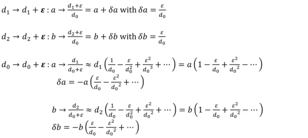
2. Statistics about the database

FIG. 5 displays the histograms of the quantities measured in our database (268 bifurcations ) and shows the distribution of the parameters describing the geometry of the bifurcation (𝑎, 𝜆) and the estimated biomarkers (𝛽_𝑑𝑒𝑣, 𝑥).

TAB. 1 gives the interval of variation, the mean and median values.

This gives us an idea of the values encountered in reality. We restrict the study domain to the intervals mentioned in the first column of TAB. 1.

(13)

FIG. 5. Statistics regarding our database

(control (green), diabetic patients (magenta), Cadasil patients (red))

Interval Mean Median

𝑑0∈ [20,130] 𝜇𝑚 74𝜇𝑚 76𝜇𝑚 𝑎 =𝑑1 𝑑0 ∈ [0.75,1.2] 0.93 0.94 𝑏 =𝑑2 𝑑0 ∈ [0.27,0.96] 0.57 0.59 𝜆𝜖[0.25,1] 0.62 0.62 𝛽𝑑𝑒𝑣∈ [−0.35; 0.63] 0.031 0.018

𝑥 ∈ [1.6; 10] 3.3 2.9 _{integrated in the statistics}Negative values are not

TAB. 1. Statistics calculated on our database (268 bifurcations)

3. Junction exponent

The junction coefficient is solution of the equation:

𝑎𝑥_{+ 𝑏}𝑥_{− 1 = 0, (𝑎, 𝑏) ∈ ]0,1[ × ]0,1[} _{Eq. 11}

FIG. 6 displays the function 𝑥 = 𝑅(𝑎, 𝑏), so the junction exponent as a function of the normalized diameters. As 𝑅 does not have an explicit analytical expression, the values for 𝑥 have been obtained through the numerical resolution of Eq. 11 over]0,1[×]0,1[, with a sampling step equal to 0.002 for 𝑎 and 𝑏. The partial derivatives 𝜕𝑅

𝜕𝑎, 𝜕𝑅

𝜕𝑏 have also been numerically calculated through

(14)

FIG. 6. Junction exponent as a function of the normalized diameters (𝑎, 𝑏).

According to FIG. 6 and FIG. 7, we observe that the slope of the function is very high for 𝑎 et 𝑏 close to one. The gradient module is also high for 𝑎 close to 1 whatever the asymmetry coefficient 𝜆. In our database, half of the normalized diameters 𝑎 takes values greater than 0.94 (FIG. 5, TAB. 1). The values taken by 𝑏 are lower, with a mean and a median of 0.57 and 0.59 respectively. The median of the asymmetry coefficients is greater than 0.6. We are therefore in a zone of strong slope of 𝑅(𝑎, 𝑏) (FIG. 7). Therefore, the estimate of the junction exponent is very sensitive to errors in the estimation of diameters.

(a) log10max (1000, √( 𝜕𝑅 𝜕𝑎) 2 + (𝜕𝑅 𝜕𝑏) 2 ) (b) log10max (10, √( 𝜕𝑅 𝜕𝑎) 2 + (𝜕𝑅 𝜕𝑏) 2 )

FIG. 7. Gradient module displayed with a logarithmic scale

3.1. Error made a single diameter

3.1.1. Case of an ideal bifurcation

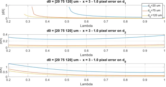
Let us consider an ideal bifurcation with 𝑥 = 3. We assume that an error of 1 pixel (𝜀 = 1) was made on one of the 3 diameters, either 𝑑0, 𝑑1 or 𝑑2. FIG. 8 shows the resulting error on the junction

exponent, as a function of the asymmetry coefficient 𝜆, and for 3 different values of the mother branch diameter 𝑑₀. These curves were obtained numerically by simulation, adding 1 pixel to one of the diameters.

(15)

FIG. 8. Error on the junction exponent for an ideal bifurcation with 𝑥 = 3,

expressed as a function of the asymmetry coefficient 𝜆, for 3 different diameters of the mother branch.

As expected (Eq. 8, Eq. 10), the smaller the caliber of the parent vessel, the higher the error on the junction exponent.

Let us give some significant examples.

• For a symmetrical bifurcation (𝜆 = 1) and a mother branch of diameter 𝑑₀ = 120𝜇𝑚 (150 pixels), an error of 1 pixel (𝜀 = ± 1) on 𝑑₀ induces an error of ±0.08 on the junction exponent (the estimate is 2.92 or 3.08 instead of 3). If the mother branch diameter is 20𝜇𝑚, the error made on 𝑥 is approximately ±0.4.

• For an asymmetric bifurcation with λ = 0.6 (median value), the errors are around ± 0.12 for a mother branch caliber 𝑑0=120𝜇𝑚 and ± 0.6 if 𝑑0=20𝜇𝑚. These results give an order

of magnitude: for an ideal bifurcation and an error of 1 pixel on the diameter 𝑑₀, 𝜆 = 0.6 (median value), the relative error made on 𝑥 is around 4% for large vessels and 20% for little ones. The same error on 𝑑1 gives an error which diverges for small vessels and very

asymmetric bifurcations. An error on 𝑑₂ is less critical, at least at this image resolution (FIG. 9).

(a) Image resolution: 0.8𝜇𝑚 (b) Image resolution: 8𝜇𝑚

FIG. 9. Error on the junction exponent for an ideal bifurcation with 𝑥 = 3,

expressed as a function of the asymmetry coefficient 𝜆, pour 3 different diameters of the mother branch. Simulations for two different image resolutions

Note the importance of image resolution: increasing the size of the pixel by a factor of 10 decreases the size of the diameters in pixels by the same factor. We can therefore conclude that the

(16)

estimation of the junction exponent is impossible on classic retinography images (FIG. 9). and maybe possible in AO for the largest vessels only.

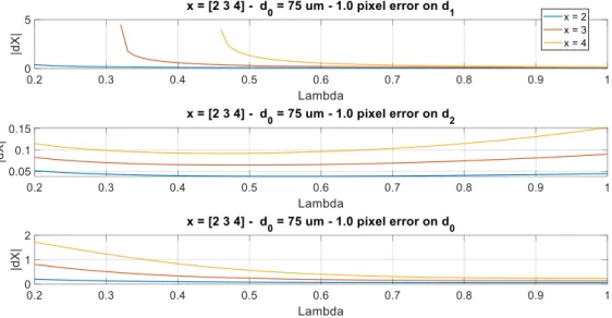
3.1.2. Case of a non-ideal bifurcation

FIG. 10 shows the same study applied for three different junction exponents. First we notice that the error increases with 𝑥, which is consistent with the slope of 𝑥 = 𝑅(𝑎, 𝑏) (FIG. 6). An error made on 𝑑₁, or to a lesser extent on 𝑑₀, is critical for small vessels and small values of 𝜆. This instability in the estimation of 𝑥 for very asymmetric bifurcations makes the deviations from an optimum 𝑥 = 3 very difficult to interpret, if not impossible.

FIG. 10. Estimation error on the junction coefficient for several values of 𝑥 expressed as a function of the asymmetry coefficient.

3.2. General case

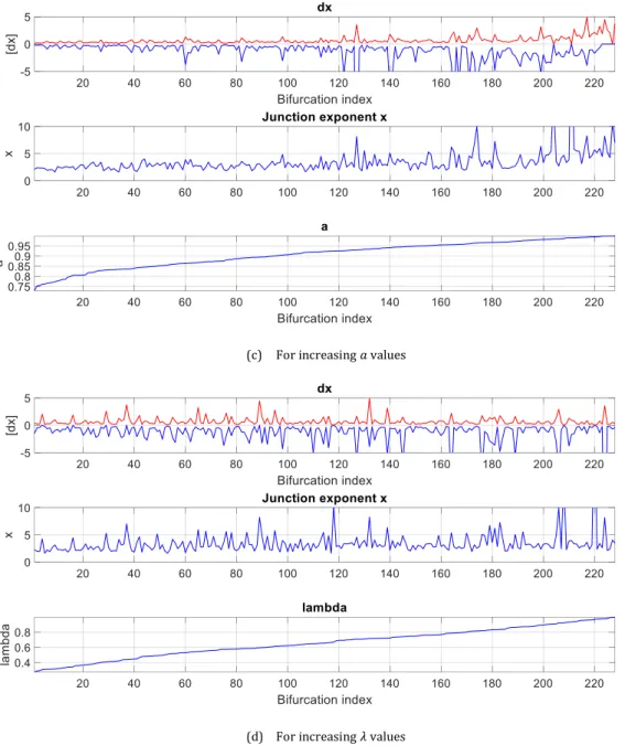
We took the measurements from our database and simulated errors made on the 3 diameters simultaneously, each one in the interval [−1, +1] pixel (sampling step: 0.1). We considered only the bifurcations with 𝑎 ≤ 1, for which we have a positive value for 𝑥 (228 bifurcations over 268). We noted the extrema of the estimation error of the junction exponent 𝑥 (maximum positive error and maximum negative error in absolute value). FIG. 11 shows the results by classifying the data according to different parameters. TAB. 2 gives statistics on the 228 involved bifurcations. We can see that these errors are important compared to the measured quantities, and very variable. Sometimes the error interval is larger than the measured junction exponent. Overall, the most important errors occur for small vessels, bifurcations with large junction exponent, and with a ratio 𝑎 = 𝑑₁/𝑑0 greater than 0.95 (which is the case for almost 30% of the database). All this is

consistent with the shape of the surface 𝑥 = 𝑅(𝑎, 𝑏) (FIG. 6, FIG. 7). This experiment also gives orders of magnitude of the error intervals, shows that these intervals vary considerably, depending on the diameter of the parent branch, the geometry of the bifurcation (a) and the true value of the junction exponent itself (𝑥). Global statistics are given in TAB. 2.

(17)

Mean Standard deviation Median

𝒙 3.46 2.37 2.92

Max positive error 0.70 0.74 0.43

Max negative error -1.36 2.50 -0.67

Interval 2.06 2.96 1.17

TAB. 2. Statistics obtained on 228 bifurcations with 𝑎 > 1

In summary, the junction exponent has very poor properties which make deviations from an optimum or differences between populations very difficult to interpret, even in high resolution imaging.

(a) For increasing 𝑑0 values

(18)

(c) For increasing 𝑎 values

(d) For increasing 𝜆 values

FIG. 11. Interval of error 𝑑𝑥 of the junction exponent 𝑥 when errors 𝜀𝑖=0,1,2 are made on the three diameters 𝑑𝑖=0,1,2

simultaneously, with 𝜀𝑖=0,1,2∈ [−1,1] pixel. Cases with 𝑎 > 1 were excluded.

4. Deviation of the branching coefficient to the optimum

As previously, we propose to study the biomarker 𝛽𝑑𝑒𝑣 as a function of the normalized diameters

𝑎 et 𝑏: 𝛽𝑑𝑒𝑣(𝑎, 𝑏) = 𝑎2+ 𝑏2− (1 + 𝜆2₎ (1 + 𝜆3₎2₃ = 𝑎2_{+ 𝑏}2₋ (1 + (𝑏_𝑎) 2 ) (1 + (𝑏_𝑎) 3 ) 2 3 Eq. 12

FIG. 12 shows 𝛽𝑑𝑒𝑣(𝑎, 𝑏). We notice that the slope is much more constant than that of the junction

(19)

estimation errors will be much more stable and not depend so strongly on the bifurcation geometry.

FIG. 12. Graphical representation of 𝛽_𝑑𝑒𝑣 as a function of the normalized diameters 𝑎 and 𝑏.

4.1. Validation of our error estimation model

We start by studying the sensitivity of 𝛽_𝑑𝑒𝑣 to an ε pixel error made on a single diameter. Then we extend to the general case of an error made on the three diameters simultaneously. This time, we have an explicit formulation of the biomarker, which allows us to perform an analytical study. Instead of working on 𝑎 and 𝑏 for a given 𝑑₀, we will express the relations as a function of 𝜆 (asymmetry coefficient) and 𝑥 (junction exponent). This makes it possible to interpret the results according to the geometry of the bifurcation, given mainly by λ, by considering ideal bifurcations for which 𝑥 = 3 or non ideal bifurcations which deviate from this optimum.

As equation 𝑑₁𝑥_{+ 𝑑} 2𝑥 = 𝑑0𝑥 is equivalent to 1 + ( 𝑑₂ 𝑑₁) 𝑥 = (𝑑0 𝑑₁) 𝑥 , we have: 𝑎 = 1 (1 + 𝜆𝑥₎_𝑥1 𝑏 = 𝜆 (1 + 𝜆𝑥₎_𝑥1 Eq. 13

Given the shape of 𝛽_𝑑𝑒𝑣(𝑎, 𝑏), we assume that a first-order model is sufficient (Eq. 8). Partial derivatives of 𝛽_𝑑𝑒𝑣(𝑎, 𝑏) are given by :

𝜕𝛽𝑑𝑒𝑣 𝜕𝑎 = 2𝑎 + 2 𝑎𝜆 2 (1 − 𝜆) (1 + 𝜆3₎5₃ Eq. 14 𝜕𝛽𝑑𝑒𝑣 𝜕𝑏 = 2𝜆𝑎 − 2 𝑎𝜆 (1 − 𝜆) (1 + 𝜆3₎5₃ Eq. 15 or:

(20)

𝜕𝛽𝑑𝑒𝑣 𝜕𝑎 = 2 (1 + 𝜆𝑥₎1_𝑥 + 2𝜆2(1 − 𝜆)(1 + 𝜆 𝑥₎1_𝑥 (1 + 𝜆3₎5₃ Eq. 16 𝜕𝛽𝑑𝑒𝑣 𝜕𝑏 = 2 𝜆 (1 + 𝜆𝑥₎_𝑥1 − 2𝜆(1 − 𝜆)(1 + 𝜆 𝑥₎_𝑥1 (1 + 𝜆3₎5₃ Eq. 17

In case of an ideal bifurcation with 𝑥 = 3: 𝜕𝛽𝑑𝑒𝑣 𝜕𝑎 |𝑥=3= 2 (1 + 𝜆2₎ (1 + 𝜆3₎4₃ _{Eq. 18} 𝜕𝛽𝑑𝑒𝑣 𝜕𝑏 |𝑥=3 = 2𝜆2 (1 + 𝜆 2₎ (1 + 𝜆3₎4₃ Eq. 19

In order to validate our model, we simulated an error of 𝜀 pixel(s) added to one of the three diameters and we calculated the resulting error made on 𝛽_𝑑𝑒𝑣. We also calculated the estimated error thanks to Eq. 8, Eq. 10, Eq. 14 and Eq. 15.

If the error of 𝜀 pixels is made on 𝑑₁:

𝛿𝛽𝑑𝑒𝑣 ≈ 𝜀 𝑑0 𝜕𝛽𝑑𝑒𝑣 𝜕𝑎 (𝑎, 𝑏) = 𝜀 𝑑0 [ 2 (1 + 𝜆𝑥₎1_𝑥 + 2𝜆2(1 − 𝜆)(1 + 𝜆 𝑥₎_𝑥1 (1 + 𝜆3₎5₃ ] Eq. 20

If the error of 𝜀 pixels is made on 𝑑₂ :

𝛿𝛽𝑑𝑒𝑣≈ 𝜀 𝑑0 𝜕𝛽𝑑𝑒𝑣 𝜕𝑏 = 𝜀 𝑑0 [2 𝜆 (1 + 𝜆𝑥₎1_𝑥 − 2𝜆(1 − 𝜆)(1 + 𝜆 𝑥₎1_𝑥 (1 + 𝜆3₎5₃ ] Eq. 21

Finally, if the error of 𝜀 pixels is made on 𝑑₀ :

𝛿𝛽𝑑𝑒𝑣 ≈ −𝑎 𝜀 𝑑0 𝜕𝛽𝑑𝑒𝑣 𝜕𝑎 (𝑎, 𝑏) − 𝑏 𝜀 𝑑0 𝜕𝛽𝑑𝑒𝑣 𝜕𝑏 (𝑎, 𝑏) = −2 𝜀 𝑑0 𝑎2(1 + 𝜆2₎ 𝛿𝛽𝑑𝑒𝑣≈ −2 𝜀 𝑑0 1 + 𝜆2 (1 + 𝜆𝑥₎2_𝑥 Eq. 22 𝛿𝛽𝑑𝑒𝑣≈ −2 𝜀 𝑑0 𝑓(𝜆), with 𝑓(𝜆, 𝑥) = 1 + 𝜆 2 (1 + 𝜆𝑥₎2_𝑥 Eq. 23

We compared the errors measured by simulation to the errors calculated thanks to the previous equations, for an ideal bifurcation (FIG. 13).

The simulated and estimated errors overlap quite well (difference of less than 2% between the simulated error and the estimated error). We could have better precision by going to order 2. In the following, we will keep the model at order 1, which seems sufficient for the analysis of the general behavior of this biomarker.

(21)

FIG. 13. Validation of our estimation model. The calculated and estimated errors overlap.

4.2. Error made on a single diameter

We analyze the partial derivatives of 𝛽_𝑑𝑒𝑣 (Eq. 16, Eq. 17, FIG. 14) mathematically as well as the function 𝑓(𝜆, 𝑥) (Eq. 23, FIG. 15), in order to determine the error interval of 𝛽_𝑑𝑒𝑣. The goal is to determine the extrema of the committed error at a given à 𝑥 (so maximization and minimization over 𝜆). This enables us to obtain a lower and an upper bound of the estimation error 𝛿𝛽𝑑𝑒𝑣 for an

ideal bifurcation (𝑥 = 3) and to analyze how these bounds evolve when a bifurcation deviates from this optimum. We restrict the study to 𝑥 ≥ 1 (TAB. 1).

FIG. 14. 𝜕𝛽𝑑𝑒𝑣

𝜕𝑎 and 𝜕𝛽𝑑𝑒𝑣

𝜕𝑏 expressed as a function of 𝜆 for a given 𝑥 (Eq. 16, Eq. 17)

(22)

Junction exponent

Error on 𝒅𝟏 Error on 𝒅𝟐 Error on 𝒅𝟎

1<𝑥 ≤ 2 21− 1 𝑥𝜀 𝑑0 ≤ |𝛿𝛽𝑑𝑒𝑣| < 2.21 𝜀 𝑑0

NB : 2.21= upper bound for any 𝑥

TAB. 3. Lower and upper bounds of |δβdev|

when a single diameter is affected by an error equal to ±𝜀 pixel(s), with 𝜀 ≥ 0

Junction exponent Error on 𝒅𝟏 Error on 𝒅𝟐 Error on 𝒅𝟎

Min Max Min Max Min Max 1 < 𝑥 ≤ 1.74 𝜆 = 1 𝜆 → 0 𝜆 → 0 𝜆 = 1 𝜆 = 1 𝜆 → 0 2 > 𝑥 > 1.74 𝜆 = 1 𝜆~0.5 𝜆 → 0 𝜆 = 1 𝜆 = 1 𝜆 → 0 𝑥 > 2 𝜆 = 1 𝜆~0.5 𝜆 → 0 𝜆 = 1 𝜆 → 0 𝜆 = 1

𝑥 = 3 𝜆 = 1 𝜆 = 0.45 𝜆 → 0 𝜆 = 1 𝜆 → 0 𝜆 = 1

TAB. 4. Values of 𝜆 that lead to the lower and upper bounds of |δβdev|.

Results are summarized in TAB. 3 and TAB. 4. TAB. 3 gives the lower and the upper bounds of the error |𝛿𝛽𝑑𝑒𝑣| made on the estimate of 𝛽𝑑𝑒𝑣 over different domains of variation of 𝑥. The particular

case of an ideal bifurcation (𝑥 = 3) is indicated in blue and represented in FIG. 16. TAB. 4 specifies the values of the asymmetry coefficient which lead to these extrema. FIG. 17 represents the extrema of TAB. 3.

FIG. 16. |𝛿𝛽𝑑𝑒𝑣| ε d0

for an ideal bifurcation (𝑥 = 3),

(23)

FIG. 17. Normalized error intervals (values reported in TAB. 3 divided by 𝜀 𝑑0)

All these results were verified by simulation, by comparing the measured errors with the calculated errors given by Eq. 20-Eq. 23. In these simulations, we fixed the junction exponent and considered a panel of parameters corresponding to the bifurcations encountered in our database (TAB. 1). We added an error of 1 pixel on a single diameter and noted the minimum and maximum errors committed on 𝛽𝑑𝑒𝑣 (FIG. 18, red and blue dots). We have also drawn the upper and lower

bounds defined in table TAB. 3 in green and cyan. We can notice that the simulation fits well the theoretical estimates.

Error on 𝒅_𝟏

(24)

Error on 𝒅𝟐

(b)

Error on 𝒅𝟎

(c)

FIG. 18. Upper and lower bounds for 𝛿𝛽_𝑑𝑒𝑣. Comparison between the simulated values (red and blue) and the calculated values (TAB. 3) derived from the differential calculus.

(25)

FIG. 19. Upper and lower bounds of the estimation error |𝛿𝛽𝑑𝑒𝑣|with respect to 𝑥 (calculated)

For a given 𝑑₀, the curves of FIG. 19 show that the error intervals do not change much with respect to 𝑥, which is a good property. This means that the confidence we can have in a measurement of 𝛽𝑑𝑒𝑣 remains the same whether the bifurcation is normal or pathological. This was not the case

for the junction exponent.

4.3. General case

4.3.1. Simulation

FIG. 20 shows the distribution of measurements made on our database, all cases involved. TAB. 1 indicates the intervals of variation of the measured quantities. This gives us the domain over which to define triplets (𝑑₀, 𝑎, 𝜆) characterizing realistic bifurcations:

• 𝑑₀∈ [20,150] 𝜇𝑚 • 𝑎 =𝑑1

𝑑0∈ [0.7,1.2]. Values greater than 1 are anomalies, but are also considered.

• 𝜆𝜖[0.2,1].

We sampled this domain with a sampling step equal to 0.2𝜇𝑚 for 𝑑0, 0.1 for 𝑎 and 0.01 for 𝜆. We

simulated errors made on the three diameters, each one within the interval [−1,1] (discrete values with a sampling step equal to 0.1, which makes in total 9261 error cases for each bifurcation (𝑑0, 𝑎, 𝜆). This way, we simulated real situations where all diameters can be affected by an

(26)

estimation error. For each bifurcation, we noted the negative and positive extrema of the error (lower and upper bounds), in order to delimit the error. These measurement errors are called the simulated bounds. They are displayed in FIG. 21 for three different calibers of the mother branch. As expected, the smaller the mother diameter, the higher the estimation errors, and the displayed surfaces exhibit some proportionality factor. The worst bifurcation geometry is for almost symmetric bifurcation with a high 𝑎 (FIG. 22). At 𝜆 fixed, the estimation error increases with 𝑎. Since the median value of this parameter is around 0.94, we are in an area of higher estimation error on 𝛽𝑑𝑒𝑣. However, we can observe in FIG. 22 that the errors are very stable over the usual

couples (𝑎, 𝜆), which is a good property: the confidence we have in a measure of 𝛽_𝑑𝑒𝑣 is the same whatever the geometry of the bifurcation. But is it inversely proportional to the diameter of the mother branch, which may lead us to restrict the clinical study to the first bifurcations in the arterial vascular tree.

FIG. 20. Measures obtained on our database (controls, Cadasil patients, diabetic patients), and isolines of 𝛽𝑑𝑒𝑣

(a) 𝑑0= 20𝜇𝑚 (b) 𝑑0= 75𝜇𝑚 (c) 𝑑0= 150𝜇𝑚

FIG. 21. Simulated lower and upper bounds of 𝛿𝛽𝑑𝑒𝑣 for several 𝑑0 diameters of the mother branch, when errors are made

(27)

FIG. 22. Lower (left) and upper(right) bounds of 𝛿𝛽_𝑑𝑒𝑣 for diameter errors 𝜀_𝑖=0,1,2∈ [−1, +1] pixel made on the three diameters 𝑑_𝑖=0,1,2 simultaneously.

In red the (𝑎, 𝜆) values taken by the bifurcations of our database with 𝑑₀∈ [90,110]𝜇𝑚.

Then we considered the measurements obtained on our database (268 triplets (𝑑0, 𝑎, 𝜆)) and we

calculated the lower and upper bounds of the error by interpolation of the simulated bounds. FIG. 23 shows the error interval found for each bifurcation of the database.

FIG. 23. Error interval (lower bound in magenta, upper bound in red) for diameter errors within [−1, +1] pixel made on the three diameters simultaneously.

4.3.2. Combined standard uncertainty

Now we seek to calculate automatically this interval of error for every estimation of 𝛽_𝑑𝑒𝑣 made on a segmented bifurcation. We will compare this calculated result to our simulated lower and upper bounds. Our method is based on the notions of standard uncertainty and combined standard uncertainty [7].

The deviation of the branching coefficient to the optimum is defined as a function of the three branch diameters 𝑑𝑖=0,1,2:

(28)

𝛽𝑑𝑒𝑣= 𝑓(𝑑0, 𝑑1, 𝑑2) = ( 𝑑1 𝑑0 ) 2 + (𝑑2 𝑑0 ) 2 − 1 + (𝑑_𝑑2 1) 2 (1 + (𝑑_𝑑2 1) 3 ) 2 3 Eq. 24

Let us denote by 𝑢(𝑑_𝑖) the standard uncertainty of 𝑑_𝑖, which corresponds to the standard deviation of the estimation error on this diameter. As we can assume that the three variables 𝑑0, 𝑑1, 𝑑2 are independant, we can estimate the combined standard uncertainty of 𝛽𝑑𝑒𝑣, denoted

𝑢(𝛽𝑑𝑒𝑣), by: 𝑢(𝛽𝑑𝑒𝑣)2= ∑ ( 𝜕𝑓 𝜕𝑑𝑖 (𝑑0, 𝑑1, 𝑑2)) 2 𝑢(𝑑𝑖)2 2 𝑖=0 Eq. 25

The partial derivatives 𝜕𝑓

𝜕𝑑𝑖 are 𝜕𝑓 𝜕𝑑0 (𝑑0, 𝑑1, 𝑑2) = − 2 𝑑0 𝑎2(1 + 𝜆2₎ 𝜕𝑓 𝜕𝑑1 (𝑑0, 𝑑1, 𝑑2) = 1 𝑑0 [2𝑎 +2 𝑎𝜆 2 (1 − 𝜆) (1 + 𝜆3₎5₃ ] 𝜕𝑓 𝜕𝑑2 (𝑑0, 𝑑1, 𝑑2) = 1 𝑑0 [2𝜆𝑎 −2 𝑎𝜆 (1 − 𝜆) (1 + 𝜆3₎5₃ ]

Let us also assume that the standard uncertainty of each diameter is 𝜀 pixels :

𝑢(𝑑𝑖) = 𝜀 Eq. 26

Then we can calculate the combined standard uncertainty of 𝛽𝑑𝑒𝑣 (Eq. 25) by:

𝑢(𝛽𝑑𝑒𝑣) = √𝛿𝛽_𝑑𝑒𝑣(0) 2+ 𝛿𝛽_𝑑𝑒𝑣(1) 2+ 𝛿𝛽_𝑑𝑒𝑣(2) 2 Eq. 27 with 𝛿𝛽_𝑑𝑒𝑣(0) = −2 𝜀 𝑑0 𝑎2(1 + 𝜆2₎ _{Eq. 28} 𝛿𝛽_𝑑𝑒𝑣(1) = 𝜀 𝑑0 [2𝑎 +2 𝑎𝜆 2 (1 − 𝜆) (1 + 𝜆3₎5₃ ] Eq. 29 𝛿𝛽_𝑑𝑒𝑣(2) = 𝜀 𝑑0 [2𝜆𝑎 −2 𝑎𝜆 (1 − 𝜆) (1 + 𝜆3₎5₃ ] Eq. 30

In fact, 𝛿𝛽_𝑑𝑒𝑣(𝑖) are the errors made on 𝛽_𝑑𝑒𝑣 when a single diameter 𝑑_𝑖 is affected by an estimation error (Eq. 20, Eq. 21, Eq. 22).

(29)

FIG. 24 shows again the simulated lower and upper bounds of 𝛿𝛽𝑑𝑒𝑣 (FIG. 23), and, in blue, the

combined standard uncertainty (and its opposite), calculated with Eq. 27 for ε=1. We can notice that the plots look very similar, to a certain factor.

FIG. 24. Simulated lower and upper bounds of 𝛿𝛽_𝑑𝑒𝑣 (magenta and red) for diameter errors 𝜀_𝑖=0,1,2∈ [−1, +1] and combined standard uncertainty (Eq. 27 - Eq. 30) for 𝜀 = 1.

Finally we look for the expanded uncertainty 𝑘𝑢(𝛽𝑑𝑒𝑣), so that, if 𝛽𝑑𝑒𝑣 is the obtained measure,

the interval [𝛽_𝑑𝑒𝑣− 𝑘𝑢(𝛽𝑑𝑒𝑣); 𝛽𝑑𝑒𝑣+ 𝑘𝑢(𝛽𝑑𝑒𝑣)] includes the true value of 𝛽𝑑𝑒𝑣. We sought this

factor 𝑘 experimentally, through a least square minimization over the 268 bifurcations of our database. The optimal value we found is 𝑘 = 1.5. The calculated errors fit then closely the simulated errors (mse = 0.014, FIG. 25).

So, the interval error can be calculated by: |𝛿𝛽𝑑𝑒𝑣|𝑚𝑎𝑥= 𝑘𝑢(𝛽𝑑𝑒𝑣) = 𝑘√𝛿𝛽𝑑𝑒𝑣 (0) 2_{+ 𝛿𝛽} 𝑑𝑒𝑣 (1) 2_{+ 𝛿𝛽} 𝑑𝑒𝑣 (2) 2 𝑘 = 1.5 Eq. 31

where 𝛿𝛽_𝑑𝑒𝑣(𝑖)_{are calculated thanks to Eq. 28, Eq. 29, Eq. 30.}

Thus, given the standard uncertainty ε on the diameter measurements, we can calculate 𝛽_𝑑𝑒𝑣 for any bifurcation (𝑑₀, 𝑑1, 𝑑2) with reliable lower and upper bounds of the true value.

We can also deduce the error interval from the lower and upper bounds calculated as a function of 𝑥 (TAB. 3), when the junction exponent is calculable (𝑎 ≤ 1).

|𝛿𝛽̅̅̅̅̅̅̅̅|𝑑𝑒𝑣 _𝑚𝑎𝑥≈ 1.325√𝛿𝛽𝑑𝑒𝑣 (0,𝑚𝑎𝑥)2_{+ 𝛿𝛽} 𝑑𝑒𝑣 (1,𝑚𝑎𝑥)2_{+ 𝛿𝛽} 𝑑𝑒𝑣 (2,𝑚𝑎𝑥)2 𝛿𝛽_𝑑𝑒𝑣(0,𝑚𝑎𝑥) = max (2, 22(1−1𝑥)₎ 𝜀 𝑑0 ; 𝛿𝛽_𝑑𝑒𝑣(1,𝑚𝑎𝑥)= 2.21 𝜀 𝑑0 ; 𝛿𝛽_𝑑𝑒𝑣(2,𝑚𝑎𝑥)= 2(1−1𝑥) 𝜀 𝑑0 Eq. 32

The estimate is less good (MSE = 0.06), but acceptable, especially for the biggest vessels. This result is not surprising since we have seen that the error intervals are stable with respect to 𝑥

(30)

(TAB. 3, FIG. 17), therefore ultimately essentially proportional to 𝜀

𝑑0. It is verified here in the

general case where errors can be made on the three diameters simultaneously. This is a very good property of this biomarker.

FIG. 25.Simulated lower and upper bounds of 𝛿𝛽𝑑𝑒𝑣 (magenta, red) and expanded uncertainty (Eq. 31),

for diameter errors 𝜀_𝑖=0,1,2∈ [−1, +1] (MSE = 0.014).

FIG. 26. Simulated error interval (magenta, red) and calculated error interval (blue) according to Eq. 32, for diameter errors 𝜀_𝑖=0,1,2∈ [−1, +1] (MSE = 0.03).

Finally, we can have a rough estimate of the lower and upper bounds of 𝛿𝛽_𝑑𝑒𝑣 for ε_i=0,1,2 ∈ [−1, +1] by:

|𝛿𝛽̅̅̅̅̅̅̅̅|𝑑𝑒𝑣 _𝑚𝑎𝑥≈

5.0 𝑑0

(31)

FIG. 27. Simulated error interval (magenta, red) and calculated error interval (blue, cyan) according to Eq. 33

for diameter errors 𝜀𝑖=0,1,2 ∈ [−1, +1] (MSE = 0.06).

5. Conclusion

The deviation of the branching coefficient from the optimum, 𝛽_𝑑𝑒𝑣, has much better properties than the junction exponent 𝑥:

• It can be calculated for any (𝑑₀, 𝑑1, 𝑑2), even if 𝑑0< 𝑑1.

• The impact of diameter estimation errors on the accuracy of 𝛽𝑑𝑒𝑣 depends little on the

geometry of the bifurcation (a, λ) or its deviation from optimality (x). The error interval is essentially proportional to 1

𝑑0, where 𝑑0 is the diameter of the parent branch expressed in

pixels.

• We can accurately calculate the error interval of each measurement of 𝛽_𝑑𝑒𝑣 by Eq. 31. We can have a pretty good approximation by Eq. 33.

Consequently, clinical studies must rely on 𝛽_𝑑𝑒𝑣 rather than on the junction exponent. However, we have now to determine whether this precision is sufficient with regard to the differences measured between control patients and pathological patients, knowing that the expected value for a normal bifurcation is 𝛽_𝑑𝑒𝑣 = 0.

Anyway, adaptive optics ophthalmoscopy images allow a much better precision in the estimation of diameters than standard retinography, as the image resolution is ten times better; so AOO images allow a much higher precision in the estimation of 𝛽_𝑑𝑒𝑣 than classical eye fundus images.

(32)

6. Rererences

[1] Lermé, Nicolas, Florence Rossant, Isabelle Bloch, Michel Paques, Edouard Koch, and Jonathan Benesty. "A fully automatic method for segmenting retinal artery walls in adaptive optics images." Pattern Recognition Letters 72 (2016): 72-81.

[2] F. Rossant, I. Bloch, I. Ghorbel, M. Pâques, Parallel Double Snakes. Application to the segmentation of retinal layers in 2D-OCT for pathological subjects, Pattern Recognition 48 (2015), pp. 3857-3870, 2015.

[3] Trimeche, Iyed, Florence Rossant, Isabelle Bloch, and Michel Paques. "Segmentation of Retinal Arterial Bifurcations in 2D Adaptive Optics Ophthalmoscopy Images." In 2019 IEEE International Conference on Image Processing (ICIP), pp. 1490-1494. IEEE, 2019.

[4] Trimeche, Iyed, Florence Rossant, Isabelle Bloch, and Michel Paques. “Fully automatic CNN-based segmentation of retinal bifurcations in 2D adaptive optics ophthalmoscopy images”, In 2020 IEEE International Conference on Image Processing Theory, Tools and Applications, (IPTA'20,) Paris, France, November 2020.

[5] Murray, C. D. (1926). The physiological principle of minimum work: I. The vascular system and the cost of blood volume. Proceedings of the National Academy of Sciences of the United States of America, 12(3), 207. [6] https://www.imagine-eyes.com/products/rtx1/

[7] Mesures et incertitudes, Ressources pour le cycle terminal général et technologique,

https://cache.media.eduscol.education.fr/file/Mathematiques/12/7/LyceeGT_ressources_MathPC_Mesure_e t_incertitudes_218127.pdf