HAL Id: halshs-00564950
https://halshs.archives-ouvertes.fr/halshs-00564950
Preprint submitted on 10 Feb 2011HAL is a multi-disciplinary open access
archive for the deposit and dissemination of sci-entific research documents, whether they are pub-lished or not. The documents may come from teaching and research institutions in France or abroad, or from public or private research centers.
L’archive ouverte pluridisciplinaire HAL, est destinée au dépôt et à la diffusion de documents scientifiques de niveau recherche, publiés ou non, émanant des établissements d’enseignement et de recherche français ou étrangers, des laboratoires publics ou privés.
Framing social security reform: Behavioral responses to
changes in the full retirement age
Luc Behaghel, David M. Blau
To cite this version:
Luc Behaghel, David M. Blau. Framing social security reform: Behavioral responses to changes in the full retirement age. 2010. �halshs-00564950�
WORKING PAPER N° 2010 - 37
Framing Social Security reform:
Behavioral responses to changes in the full retirement age
Luc Behaghel David M. Blau
JEL Codes: J26
Keywords: Social security, framing, loss aversion, retirement
P
ARIS-
JOURDANS
CIENCESE
CONOMIQUES 48,BD JOURDAN –E.N.S.–75014PARISTÉL. :33(0)143136300 – FAX :33(0)143136310 www.pse.ens.fr
CENTRE NATIONAL DE LA RECHERCHE SCIENTIFIQUE –ECOLE DES HAUTES ETUDES EN SCIENCES SOCIALES
Framing Social Security Reform:
Behavioral Responses to Changes in the Full Retirement Age.1
Luc Behaghel (Paris School of Economics-INRA)2
David M. Blau (Ohio State University)3
First draft: March 2010; current draft: November 2010
Abstract
We use a US Social Security reform as a quasi-experiment to provide evidence on framing effects in retirement behavior. The reform increased the full
retirement age (FRA) from 65 to 66 in two month increments per year of birth for cohorts born from 1938 to 1943. We find strong evidence that the spike in the benefit claiming hazard at 65 moved in lockstep along with the FRA. Results on self-reported retirement and exit from employment are less clear-cut, but go in the same direction. The responsiveness to the new FRA is stronger for people with higher cognitive skills. We interpret the findings as evidence of reference dependence with loss aversion. We develop a simple labor supply model with reference dependence that can explain the results. The model has potentially important implications for framing of future Social Security reforms. JEL: J26
1
The research in this paper was conducted while the second author was a Special Sworn Status researcher of the U.S. Census Bureau at the Triangle Census Research Data Center. Any opinions and conclusions expressed herein are those of the author(s) and do not necessarily represent the views of the U.S. Census Bureau. All results have been reviewed to ensure that no confidential information is disclosed. Financial support from NIA grant P30-AG024376 and NSF-ITR grant #0427889 is gratefully acknowledged. We thank Sudipto Banerjee for research assistance. We appreciate helpful comments from seminar participants at MRRC, PSE, and NBER, and from Jonathan Zinman. We are grateful for
especially detailed comments from Joe Doyle. The authors are solely responsible for the contents.
2
3
1. Introduction
Understanding the labor force, benefit take up, and saving decisions of older workers has
become increasingly important in today’s environment of rapid population aging and large Social
Security financial imbalances. The life cycle model provides a powerful framework for modeling
retirement decisions, and has been the basis for a substantial amount of informative and
policy-relevant research. But some aspects of retirement behavior have proven difficult to explain in the
life cycle framework. These include failure to take up employer-provided defined contribution
pension plans that provide very favorable terms such as a generous employer match (Madrian
and Shea, 2001), and lack of knowledge of pension provisions (Chan and Stevens, 2008).
Another feature of retirement behavior that seems hard to reconcile with a life cycle approach is
the persistence of large spikes in exit from the labor force and take up of Social Security benefits
(Old Age and Survivors Insurance, or OASI) in the US at age 65. Costa (1998) shows that there
was little evidence of a spike in labor force exit in the 1900-1920 period, but a spike at age 65
had emerged by 1940, five years after the establishment of Social Security. The size of the spike
was as high as 30% on an annual basis in the mid 1980's (Perrachi and Welch, 1994), and
declined to 19% in the 2000's.4
Several explanations for the age 65 spike that are consistent with the life cycle framework
have been proposed. These include (1) a liquidity constraint that makes it difficult financially for
some low income workers to retire before becoming eligible for Social Security benefits, (2) a
kink at age 65 in the schedule that determines the Social Security benefit as a function of the age
4
Source: author’s calculations from the Health and Retirement Study, described below. A new spike in the hazard rates of labor force exit and benefit claiming emerged after 1962, when early Social Security entitlement at age 62 became available (Moffitt, 1987). Note that exiting employment and claiming the OASI benefit are distinct choices, although they are closely related in practice. The spikes in
2 of claiming, (3) the prevalence of age 65 as the normal age of retirement in many Defined
Benefit (DB) pension plans, and (4) loss of health insurance coverage as a result of retiring
before becoming eligible for Medicare at age 65. The evidence on these explanations (discussed
below) is mixed, but overall it suggests that these factors cannot account for more than a small
portion of the spike in retirement at 65, either alone or in combination. The evidence is not
conclusive, however, because some of these explanations cannot be directly tested.
Other explanations for the age 65 spike have been proposed in the behavioral economics
framework, in which the assumptions of farsighted rational behavior and standard preferences
are relaxed. 65 was designated as the Full Retirement Age (FRA) from the beginning of the
OASI program until recently. Workers might take this “official” designation as implicit advice
from the government about when to retire and claim benefits, and as a result retirement at age 65
may have become a social norm. Information provided by the Social Security Administration
(SSA) on their web site and in individualized “accounting reports” sent directly to future
beneficiaries is explicitly framed with reference to the FRA. To paraphrase: Your FRA is 65. If
you continue to work until 65, your monthly benefit will be $X. If instead you claim at age 62,
your benefit will be 80% of X. If you postpone claiming until age 70, your benefit will be 130%
of X. This presentation could lead to framing effects at 65, resulting in age 65 becoming a
reference point. There is little direct evidence to date on behavioral economic explanations for
the age 65 spike. Most of the evidence comes from testing and rejecting other explanations,
leaving behavioral economic explanations as the default (Lumsdaine, Stock, and Wise, 1996).
3 A Social Security reform enacted into law in 1983 increased the FRA from 65 to 66 in
two month increments per year of birth for cohorts born from 1938 to 1943.5 The cohorts
affected by the reform reached their FRA in 2004-2009, so data on their retirement behavior are
becoming available now. This provides an unusual opportunity to test both life-cycle and
behavioral economic explanations for the age 65 spike. The increase in the FRA is equivalent to
a cut in the Social Security benefit: claiming the benefit at any given age results in a lower
benefit than if the FRA had not changed. This reduces the expected present discounted value of
lifetime benefits (Social Security Wealth), and should cause an increase in the age of retirement
if leisure is a normal good. But, as illustrated in Figure 1, the increase in the FRA did not change
the slope of the benefit-claiming-age schedule in the vicinity of the FRA.6 So there is no
economic incentive for someone who, for whatever reason, would have retired or claimed the
benefit at 65 if the FRA had not changed, to instead do so at his new FRA of 65 and 2 months, or
65 and 4 months, etc. If the spike in retirement or benefit claiming at age 65 shifts across cohorts
in parallel with the increase in the FRA, explanations based on the standard life cycle framework
would be unable to account for this. This would point toward behavioral economic explanations.
Our first contribution in this paper is to estimate the effect of the increase in the FRA on
the hazard of exiting employment and the hazard of claiming the OASI benefit. Several recent
5
The FRA is 65 for cohorts born before 1938, 65 and 2 months for the 1938 birth cohort, 65 and 4 months for the 1939 birth cohort, etc., and 66 for cohorts born from 1943-1954. A similar stepwise increase from 66 to 67 for cohorts born from 1955 to 1960 was also mandated.
6
The implied benefit cut is the same at all claiming ages up to and including the FRA except between 62 and 63. The benefit cut implied by a one year increase in the FRA is 5% if the benefit is claimed between 62 and 63, and 6.67% if the benefit is claimed between 63 and 66. Another reform enacted in 1983 gradually increased the Delayed Retirement Credit (DRC), the slope of the benefit-claiming-age profile after the FRA, from 1% for those turning 62 in 1981 to 8% for those turning 62 in 2005. The benefit cut implied by a one year increase in the FRA for an individual who claims the benefit
4 studies have estimated the effect of the increase in the FRA on the timing of labor force exit or
benefit claiming (Blau and Goodstein, 2010; Kopczuck and Song, 2008; Mastrobuoni, 2009;
Pingle, 2006; Song and Manchester, 2008), but none have focused specifically on the impact on
the spike in retirement at 65. In the first part of the paper, we use data from the Health and
Retirement Study (HRS) and the Longitudinal Employer-Household Data (LEHD) to analyze
changes in the retirement and claiming hazards across cohorts. We find strong evidence that the
spike in the OASI benefit claiming hazard moved in lockstep along with the FRA, consistent
with findings from administrative data (Song and Manchester, 2008). Results on self-reported
retirement and exit from the labor force are less clear-cut: we find evidence that the spike in
labor force exit at 65 decreased substantially and in some cases vanished for cohorts whose FRA
increased, but less systematic evidence that new spikes have appeared at the new FRAs. The
difference between effects on claiming and labor force exit may indicate that the change in the
FRA is less salient for leaving employment than for claiming. Depending on the outcome we
examine, the FRA effect can account for 10 to 40% of the initial hazard at age 65.
These results add to the growing literature on evidence “from the field” in behavioral
economics. By contrast with other applications of framing effects to labor supply, the FRA offers
a particularly favorable setting: the reference is explicitly defined and then exogenously modified
by the 1983 reform, so that the behavioral component is clearly identified from cohort
discontinuities. 7
Our second contribution is to address the novel question of “who is behavioral”
(Benjamin, Brown, and Shapiro, 2006) with respect to age of retirement. This is important in
5 order to infer which of several potential behavioral economic explanations is most consistent
with the results. We define a group of workers as behavioral if the group’s claiming and labor
force exit behavior closely parallels the shift in the FRA. We define groups in several ways: by
(1) socioeconomic characteristics such as gender, education, race, and marital status; (2) job
characteristics; (3) cognitive ability; (4) financial literacy and planning horizon; and (5)
non-cognitive characteristics such as risk aversion and subjective expectations about longevity. The
most consistent finding is that workers with higher cognitive respond more strongly to the FRA
change. One might have expected that low cognitive skills would make an individual more likely
to interpret the change in the FRA as advice from the SSA. However, the most plausible
explanation for the evidence we find is reference dependence, which is a form of non standard
preferences, as opposed to non standard decision making such as might result from low cognitive
skill. Moreover, the lower FRA effect for workers with low cognitive ability is largely due to the
persistence of a large spike at age 65 for this group after the reform. This suggests that people
with lower cognitive skills may be slower to learn about the FRA change or to integrate the new
reference point in their claiming decision, perhaps instead keeping workers from earlier cohorts
as their reference. To summarize, both groups of workers would be “behavioral” in the sense of
reacting to a reference point with loss aversion, but workers with lower cognitive skills would be
slower to adjust to the new reference points.
The evidence we present is of inherent interest for understanding retirement behavior, but
it could also have important implications for future Social Security policy. To illustrate these
implications, we develop a simple behavioral model of retirement that incorporates reference
7
For a survey of empirical applications, see Della Vigna (2009); for theoretical solutions to the indeterminacy of the reference point, see for instance Koszegi and Rabin (2006).
6 dependence and loss aversion. The model is used to demonstrate that reference dependence can
amplify or dampen the impact on the average age of retirement caused by a reform such as a
change in the FRA, depending on how the reform is framed. Simulations of the model for
plausible parameter values indicate that the manner of framing a policy reform can have a
sizeable effect on its impact on retirement behavior in the presence of reference dependence.
The next section of the paper briefly reviews previous findings and places our
contribution in context. The following section describes the data, and sections 4 and 5 present
evidence on the effect of the shift in the FRA. Section 6 analyzes the question of “who is
behavioral?” Section 7 describes and analyzes the implications of a simple behavioral model of
retirement. The final section concludes.
2. Background and Previous Studies
Here, we briefly review evidence on explanations for the age 65 spike that are consistent
with the standard life cycle model.
(1) Liquidity Constraint. Until 1962, eligibility for OASI began at age 65. Low income
workers who saved little during their working years could face a liquidity constraint that makes it
difficult to finance consumption during retirement before receiving the OASI benefit. This could
explain the prevalence of retirement at the earliest age of eligibility. However, the earliest age of
eligibility for OASI was changed to 62 in 1962, but the spike at age 65 remained and even grew,
thus providing evidence against a liquidity constraint explanation. It is possible that liquidity
constraints were an important source of the spike before 1962 and were gradually supplanted by
7 (2) Nonlinear Budget Set. Until the 1990s there was a sharp kink at the FRA in the
schedule that determines the Social Security benefit as a function of the age of claiming.
Delaying claiming from 62 to 65 resulted in an approximately actuarially fair benefit increase
(6.67% per year), but delaying claiming past 65 resulted in a much less than actuarially fair
increase (1% up to 1981; 3% from 1981 until 1989). The age-65 spike could be rationalized as a
response to a kinked intertemporal budget constraint. However, the 1983 Social Security reforms
eliminated the kink, gradually increasing the reward to delaying claiming past the FRA from 3%
for cohorts reaching their FRA in 1989 to 8% for cohorts reaching their FRA in 2008. By the
mid-2000's there was no longer a kink in the benefit-claiming age schedule, and today there is
even a slight convex kink, yet the spike in retirement at age 65 for cohorts with an FRA of 65
persisted, suggesting that the budget constraint kink was not the main factor behind the age 65
spike in retirement, at least in recent years.
(3) Defined Benefit Pensions. DB pension plans often have a normal retirement age of
65, and these plans usually have very strong incentives to retire by the normal age (conditional
on not having retired at the earliest age of eligibility, which is typically quite attractive as well).
DB pensions are much less common today, having been largely supplanted by Defined
Contribution (DC) plans.8 DC plans do not have any incentives to retire at 65 or any other
particular age. However, the switch from DB to DC plans affected the cohorts reaching their mid
60’s in the 2000s much less than it has affected more recent cohorts. The prevalence of DB
8
Measured in terms of annual contributions by employers, DB plans accounted for 60% of total private sector employer contributions in 1980, and only 13% in 2000 (Poterba, Venti, and Wise, 2007). DB plans remain prevalent in the public sector.
8 pension coverage in these older cohorts is consistent with the persistence of the age 65 spike. We
control for DB pension coverage and, for those with DB plans, the normal retirement age.
(4) Health Insurance. Workers who would lose their employer-provided health insurance
upon retiring might prefer to postpone retirement until Medicare eligibility at age 65 in order to
avoid being uninsured, leading to a spike in retirement at 65. The age of eligibility for Medicare
has been 65 since the program was introduced in 1965, so there is no direct evidence on this
explanation, although the age-65 spike was present before 1965. It is possible that Medicare has
replaced the other explanations for the age-65 spike as they have become less relevant, but this is
difficult to determine because of the lack of variation in the Medicare eligibility age.9
The most plausible behavioral economic explanation for the age 65 spike stems from the
fact that 65 was the Social Security FRA until recently. The FRA is not presented as a norm – the
SSA presents things in a balanced way: “If you retire early, you may not have enough income to
enjoy the years ahead of you. Likewise, if you retire late, you’ll have a larger income, but fewer
years to enjoy it. Everyone needs to find the right balance based on his or her own
circumstances.” (SSA, 2008a). However, in personalized Social Security statements the FRA is
explicitly used as a reference in a bar chart illustrating benefits as a function of claiming age.10
Moreover, the distinction between retiring “early” (that is, earlier than the FRA) and retiring
9
Evidence on the role of Medicare in retirement decisions derived from simulations based on structural models is provided in Rust and Phelan (1997) and Blau and Gilleskie (2006, 2008). Rust and Phelan conclude that Medicare was an important determinant of retirement timing in the 1970s, while Blau and Gilleskie conclude that it was much less important in the 1990s.
10
See Mastrobuoni (2010) for discussion of the history of the Social Security statement and the impact of its introduction on retirement behavior.
9 “late” (later than the FRA) is explicitly discussed (SSA, 2008b; see appendix). Clearly, the way
the FRA is used in framing benefits invites people to use it as their point of reference.11
There is little direct evidence on the explanatory power of specific behavioral economic
explanations for the age 65 spike. Featherstonehaugh and Ross (1999) and Liebman and Luttmer
(2009) pose hypothetical questions to survey respondents to gauge the importance of framing
effects in the presentation of information about Social Security. Framing effects appear to matter
at some ages and not at other ages, but the scenarios are hypothetical. The hypothetical
experiment we have in mind would cut Social Security benefits by a given amount, and frame
the cut in alternative ways: (1) as a neutral across-the-board cut irrespective of the age at which
the benefit is claimed, (2) as a cut in the benefit available at a particular reference age, holding
constant the slope of the benefit-claiming-age profile, and (3) as an increase in the age at which a
given reference benefit level is available, again holding the slope constant. In each scenario,
individuals would be perfectly well informed about the cut, and capable of determining their
optimal response, given their preferences. This would eliminate lack of information and limited
cognitive ability as confounders, so any differences in responses across scenarios could be
attributed to reference dependence. The actual quasi-experiment induced by the reform did hold
the benefit-claiming-age profile roughly constant (c.f. Figure 1), and used framing option 3 (an
increase in the FRA). We cannot compare results for different framing options and we cannot
rule out information and cognitive ability as confounders. We discuss indirect approaches to
assessing the importance of these issues in sections 5 and 6.
11
This is true for cohorts with non-integer FRAs. For instance, for workers born in 1939, the statement reads: “The earliest age at which you can receive an unreduced retirement benefit is 65 and 4 months.”
10 Recent evidence indicates that the increase in the FRA has affected retirement behavior.
Mastrobuoni (2009) analyzed the age of exit from the labor force of the “treated” cohorts,
comparing them to earlier cohorts not affected by the increase in the FRA. His estimates indicate
that each two month increase in the FRA caused a one month increase in retirement age. Blau
and Goodstein (2010) and Pingle (2006) also estimate that the increase in the FRA has caused an
increase in employment at older ages. The evidence in these three studies does not address the
mechanism through which the FRA effect operates, and therefore does not shed light on the
question of why the FRA has affected retirement behavior. The evidence is consistent with a
wealth effect that would alter behavior at all ages, but it does not address the question of whether
there is a shift in the spike at age 65.
In contrast, recent evidence on Social Security claiming clearly suggests a behavioral
economic interpretation. There is no economic incentive to claim the OASI benefit at the FRA,
yet that is precisely what the treated cohorts have done. Song and Manchester (2008) and
Kopczuck and Song (2008) use administrative data to show that the increase in the FRA has
caused the spike in claiming at age 65 to shift almost completely to the new FRA for the affected
cohorts. This finding is difficult to explain in the life cycle framework. The key unanswered
questions that we seek to address are whether there is similar evidence for employment; if so,
how can we explain it; and who is “behavioral.”
3. Data
Previous studies of the impact of the FRA have used data from the Current Population
11 Participation (Pingle, 2006), and SSA administrative data (Song and Manchester, 2008; Kopczuk
and Song, 2008). These data sources provide large sample sizes, which may be needed to detect
the effects of small changes in the FRA (two months per birth cohort). We use data from the
Health and Retirement Study (HRS), which provides a rich set of potential explanatory variables
to study behavioral aspects of retirement. These variables are unique to the HRS and offer the
opportunity to get closer to explaining behavioral aspects of retirement as well as documenting
their existence.
The main disadvantage of the HRS is the relatively small samples available to study
retirement and claiming behavior at the FRA. Roughly three quarters of workers retire and claim
benefits before reaching the FRA, so despite sample sizes of about 1,000 respondents per year of
birth, the effective sample size is closer to 250 per cohort. This provides about 1,125
observations on the treated cohorts, and 1,750 for the control cohorts. Therefore, we also use
data from the Longitudinal Employer-Household Data (LEHD) files. These files are derived
from administrative state Unemployment Insurance (UI) records, with very large sample sizes.
These administrative data are used only for descriptive purposes to verify that the trends
identified in the HRS are robust, since they contain no information on any of the explanatory
variables of interest. The LEHD is described in Section 4.
The HRS is a biennial survey of a sample of households containing individuals over the
age of 50, and their spouses. The survey began in 1992 with birth cohorts 1931-1941, and new
cohorts were added in 1998 and 2004. We use the 1992-2008 waves. The analysis sample is birth
12 not. The 1931-37 cohorts are the controls (FRA=65.0) and the 1938-42 cohorts are the treated
cohorts (FRA>65.0).
The HRS records employment status at each interview, and in addition asks for
information on the start and end dates of all jobs between interviews, to the nearest month. We
construct a monthly employment history.12 Together with month and year of birth, the
employment data are used to construct the month and year of labor force exit.13
The HRS contains self-reported information on the month and year in which the
respondent first received a Social Security benefit payment. In some cases, the reported date is
before the respondent turned 62, indicating that he or she first received some type of Social
Security benefit other than OASI, such as disability or dependent benefits. In these cases it is not
possible to identify when the respondent claimed the OASI benefit.14 The month and year of
OASI claiming is the second outcome of interest.
A third outcome of interest is the self-reported month and year of retirement. This
“subjective” measure is frequently used as an indicator of retirement, and it is of interest to
determine whether “retirement” and “employment” differ with respect to the FRA. However,
there are many longitudinally inconsistent self-reports of retirement age, so only about half the
sample has a self-reported retirement age that is reasonably consistent across waves.
12
The initial interview collected information on the start date of the job held at the interview date, start and end dates of up to two other jobs before the first interview (longest and last), and the number of additional jobs that lasted five or more years.
13
Some people who leave the labor force later return to employment. In such cases there are multiple labor force exit dates. As a robustness check, we use labor force exits that are preceded by an employment spell of at least 3 months, and followed by at least 3 months out of employment.
14
If an individual reaches his FRA while receiving Social Security Disability Insurance, the benefit is switched to OASI, but this is purely an administrative adjustment, so it does not provide any information about claiming behavior. Most SSDI recipients never leave the SSDI rolls, and therefore
13 The monthly record is merged with permanent characteristics such as race, gender,
ethnicity, and education, and with time-varying measures recorded at the survey dates, including
health status, the wage rate, job characteristics, household wealth, health insurance, pension
coverage, and marital status. If there was a change in one of these time-varying variables
between waves, we assume the change occurred midway between the waves.
The HRS contains several variables that are useful in inferring “who is behavioral”.
These include measures of cognitive ability, risk aversion, self control, and financial planning
horizon. Cognitive ability measures have been explored by McArdle, Smith and Willis (2009),
and we follow their approach to construct indicators in three dimensions: Telephone Interview of
Cognitive Status (TICS), short term memory, and numeracy (see data appendix for details).
4. Impact of the FRA increase HRS Results
In this section, we describe evidence from the HRS on how the change in the FRA has
modified the timing of OASI benefit claiming, labor force exit, and self-reported retirement. The
goal is to test the “behavioral” prediction that the spike at age 65 should shift along with the FRA
for cohorts born after 1937, against the null hypothesis that the increase in the FRA had only a
wealth effect. In the latter case we expect an increase in retirement age, but no substantial shift
in the spike.
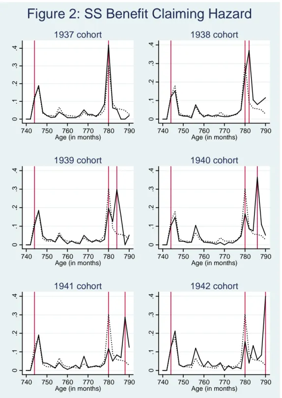
We start with graphical evidence on the timing of OASI benefit claiming across cohorts,
pooling men and women. Figure 2 displays average monthly claiming hazard rates for pre and
14 post-reform cohorts. The claiming hazard rate is defined as the probability of claiming at a given
age, conditional on not having claimed previously. Age is measured at a bimonthly frequency;
e.g. age 65 denotes age 65 0/12 to 65 1/1215 . In each graph of figure 1, the dotted line depicts the
claiming hazard for workers born between 1931 and 1936. As shown by previous studies, there
is a first spike in the hazard at or just after the early retirement age (62) and a second larger spike
at the FRA (65).16 About 20% of workers claim at the early retirement age, and 30% of those
who have not claimed before 65 claim at 65. For each cohort, the vertical lines indicate age 62,
age 65, and the FRA (if different from age 65). There is clear evidence that the spike in the
claiming hazard moves in lockstep along with the FRA. The spike at age 65 does not completely
disappear for the treated cohorts, but it becomes progressively smaller across cohorts. Very
similar patterns appear when men and women are disaggregated (not shown). These results
confirm the findings of Song and Manchester (2008), using administrative data.
Regression analysis is useful here to summarize the graphical evidence and to
quantify the impact of the FRA. We adopt the following difference-in-difference specification:
Piac =
θ
FRAiac +xiacγ
+β
a +δ
c +ε
iac (4.1) where Piac is an indicator variable equal to one if individual i born in cohort c claims at age a (inmonths), conditional on not having claimed previously. FRA is the indicator variable for age a
being his FRA, xiac is a set of individual controls, and full sets of cohort and age dummies are
15
One reason for measuring age at a bimonthly frequency is to make the graph easier to read. It is also useful because there is some arbitrariness in measuring the age at which an event occurs. If an individual reports leaving his job in April, it is not clear whether to classify his employment status in April as employed or not employed, without knowing the exact date.
16
The spike at age 62 is slightly after age 62 because benefits are payable beginning in the first month in which a person is 62 throughout the whole month, unless the person was born on the 1st or 2nd of the month (see Kopczuk and Song, 2008, for discussion).
15 included (
β
a,δ
c).The age 65 coefficient (one of theβ's) captures the part of the spike that is notexplained by the fact that 65 is the FRA for cohorts up to 1937. The parameter of interest θ is identified by the interaction of age and cohort, under the assumption that the control variables
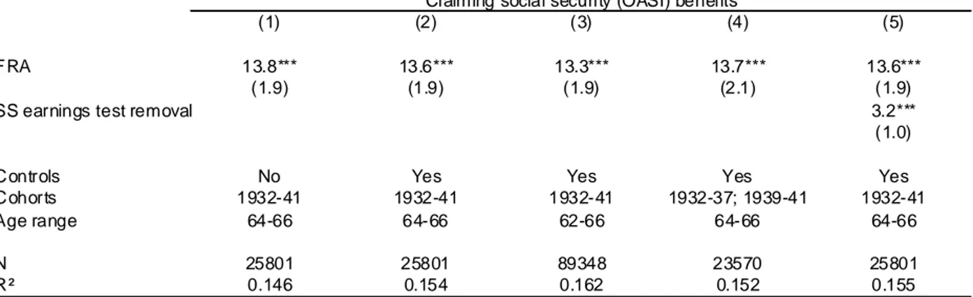
capture any non-FRA-related motives to claim at the FRA. Results are shown in table 1. The four
columns differ by the estimation sample or the controls. Column 1 has no controls other than age
and cohort effects, and restricts the analysis to ages 64 to 65 11/12. Reaching the FRA increases
the claiming hazard by 14 percentage points. The effect is statistically highly significant, and
robust to the inclusion of controls (socioeconomic characteristics, pension and job
characteristics, measures of cognitive ability, planning horizon and risk aversion) and to changes
in the estimation sample (columns 2 to 4). Column 4 drops the 1938 cohort since the graphical
analysis suggests that the effect of the FRA change might have been smaller for that cohort (with
a higher persistence of the old FRA spike), possibly due to a learning effect. This however makes
little difference in the estimation. Quantitatively, the estimated impact of the FRA is sizeable: the
claiming hazard at age 65 is around 30% for cohorts born between 1931 and 1937; more than
40% (14/30) of the claims occurring at that age for the control cohorts can therefore be explained
by the fact that 65 is their FRA.
Equation (4.1) relies on the identifying assumption that any change in the shape of the
claiming hazard can be attributed to the FRA increase. Other changes over the period may also
have affected the timing of claiming decisions17. In particular, the Social Security earnings test
for people who have reached their full retirement age was eliminated in 2000. The rule before
17
As noted above, the 1983 reform increased the Delayed Retirement Credit (DRC) as well as the FRA. An increase in the reward to claiming the benefit after the FRA could affect claiming behavior (and
16 2000 was the following: workers who have not reached the FRA have their earnings reduced by
$1 for every $2 earned beyond the earnings test threshold; workers who have reached the FRA
have their benefits reduced by $1 for every $3 earned beyond the earnings test threshold (see
Manchester and Song, 2008). Although this reduction is compensated by increased benefits at
older ages (making it more or less neutral in terms of SS wealth), it may be felt as a disincentive
to claim benefits by those who intend to continue working (Friedberg, 2000; Gruber and Orszag,
2003; Haider and Loughran, 2008). In 2000, the earnings test was eliminated for workers who
have reached the FRA. The earnings test was unchanged before the FRA. The introduction of
this discontinuity may generate a spike in the claiming hazard around the FRA, if some workers
delay claiming SS benefits until they reach the FRA, in order to avoid the earnings test.
Fortunately, the cohorts impacted by the increase in the FRA and the removal of the earnings test
do not fully overlap, making it is possible to separately identify the two effects (see Song and
Manchester, 2008, for details). It is therefore possible to extend equation (4.1) to separately
identify the impact of the earnings test removal:
Piac =θFRAiac +λETRiac +xiacγ +βa +δc +εiac, (4.2) where ETR is an indicator for the month in which the earnings test ceases to apply to iac
individual i. The results are given in column (5). The coefficient on the FRA remains unchanged.
The impact of the earnings test removal is positive and significant, as expected, suggesting that
part of the age 65 spike for some cohorts was due to the removal of the earnings test. However,
the impact of reaching the FRA itself is much larger.
does, according to Blau and Goodstein, 2010, and Pingle, 2006). But the DRC is cohort-specific, so its effects are absorbed by cohort dummies.
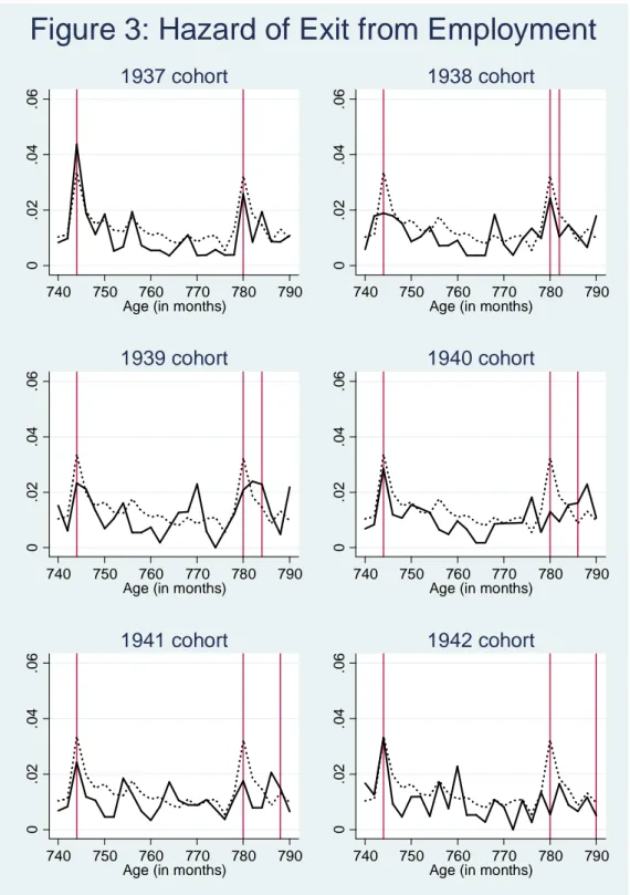
17 As shown by Coile et al. (2002) and Baker and Benjamin (1999), benefit claiming
behavior can significantly differ from labor force participation and retirement behavior. Before
interpreting the shift in the claiming spike from a behavioral perspective, it is therefore important
to check whether retirement and employment patterns are similar to claiming patterns. Figure 3
shows that the increase in the FRA resulted in a progressive fall in the age 65 spike in the labor
force exit hazard. However, there is no systematic evidence of new spikes at the FRA for cohorts
born after 1937.
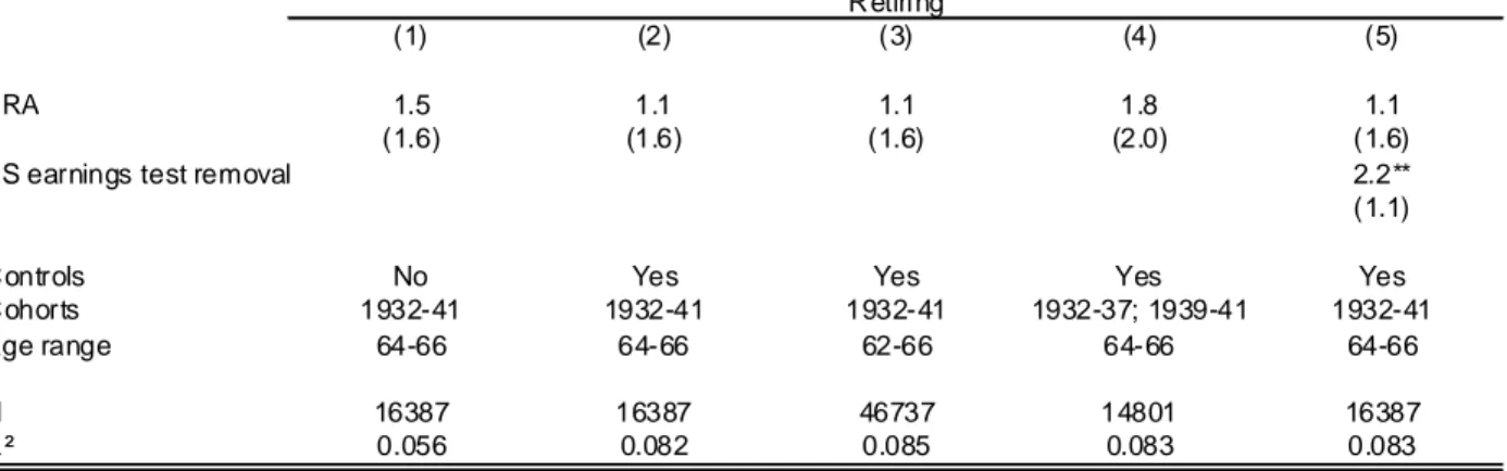
Columns 1 to 5 in table 2 use the same specifications as table 1. The impact of the FRA is
smaller than for claiming, but is positive and significantly different from zero. For cohorts born
before 1937, the monthly hazard of labor force exit at age 65 is about 4.6%. Roughly 20% of this
spike (0.9/4.6) can be explained by the fact that 65 is the FRA for these cohorts.18 The FRA
effect is again robust to inclusion of a control for elimination of the earnings test.
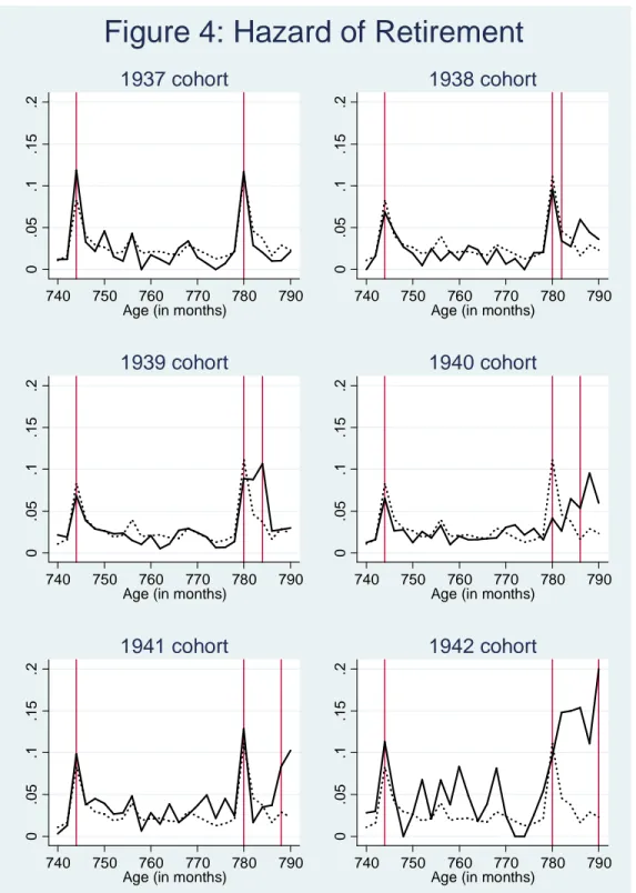
Figure 4 presents evidence on the monthly hazard of entry to self-reported retirement,
comparable to figures 2 and 3. The results are in between. There is some reasonably strong
evidence of a shift in the spike for cohorts born after 1939, consistent with an effect of the FRA
on retirement decisions. However, the spike at the old FRA (age 65) persists for some of these
cohorts. The regression results (table 3) are very imprecise. The point estimate implies a smaller
FRA impact than for claiming and exit from employment. The mean monthly retirement hazard
for the control cohorts at age 65 is around 13%. 10% of this spike (1.1/13) can be accounted for
by the fact that 65 is their FRA. The results are robust to controlling for the elimination of the
earnings test, but in this case the effect of the earnings test is larger than the effect of the FRA.
18
Results based on a smaller sample that eliminates temporary withdrawals from the labor force (three months or less) gave very similar results.
18
LEHD results
In this section, we describe evidence from the LEHD on how the change in the FRA has
affected the timing of labor force exit. The LEHD Infrastructure File system is based on state
Unemployment Insurance (UI) administrative files, with data available from 31 states covering
about 80% of the U.S. work force for the years 1990-2004, although the period covered varies by
state (Abowd, Haltiwanger, and Lane, 2004). Employers covered by UI file a quarterly report for
each individual who received any covered earnings in the quarter. UI covers about 96% of
private non-farm wage-salary employment, with lower coverage of agricultural and government
workers, and no coverage of the unincorporated self-employed. The UI records contain the
individual’s Social Security number, and an identification number and quarterly earnings for
each employer from which he has any covered earnings during the quarter. These data are
merged by the Census Bureau with the Census Personal Characteristics File, which contains the
exact date of birth, place of birth, sex, and a measure of race/ethnicity.19
The main advantage of the LEHD for our analysis is the very large sample size. The main
disadvantages are absence of information on hours of work, and lack of data after the third
quarter of 2004. Without data on hours of work, we must use changes in quarterly earnings to
infer changes in employment status. The absence of data beyond the third quarter of 2004 means
19
An extensive discussion of the construction and the content of these files is provided in Abowd et al. (2006). We use a subsample of the full LEHD files, consisting of workers who were employed at any employer at which a member of the 1990-2001 panels of the Survey of Income and Program
Participation (SIPP) worked. This is a very large subsample of the full LEHD, somewhat skewed toward large firms. See Blau and Shvydko (in press) for a description of the subsample. In order to reduce the number of quarterly observations from the hundreds of millions to the more manageable level of several
19 that only two of the “treated” birth cohorts (1938 and 1939) can be used to analyze changes in
labor force behavior around age 65..
The main outcome of interest is a binary indicator of zero earnings in a given quarter,
conditional on positive earnings in the previous quarter, which we interpret as the hazard of labor
force exit. We aggregate the data into cells defined by month and year of birth (January 1931
through December 1942), calendar quarter (1994:Q1 through 2004:Q3, although not all quarters
are represented for all cohorts), and age in quarters (62.0, 62.25, 62.5,..., 66.0), and conduct the
analysis using cell means, with no loss of information. Data are available for 2,400 cells, with
roughly 1,000 individual observations per cell on average. Men and women are pooled and
gender and state dummies (fractions, after aggregation) are included in the regression models.
The specification used in column 1 of table 4 is the same as in tables 2-4. Age and birth
year dummies are included, so that the effect of the FRA variable is identified from the
interaction of age and birth cohort.20 The results are consistent with reference dependence, with a
positive FRA effect on the exit hazard, significantly different from zero. Given the fact that the
data only has two post-reform cohorts, we check a new specification in column 2. The FRA
indicator is interacted with cohort dummies: so, the coefficient on the FRA*(coh=1938) variable
can be interpreted as the average impact of the FRA for cohort 1938, compared to individuals of
the same age in the 1931-37 cohorts, and accounting for cohort trends. The results are
million, we use data from only three states. Census Bureau guidelines prevent us from identifying the three states.
20
If a worker leaves employment at his FRA, his earnings will be positive in the quarter in which his FRA falls (unless he quits on the first day of the quarter), so zero earnings in the first calendar quarter after the quarter in which he reaches his FRA is the only reliable measure of exit at the FRA. Depending on birth month within a quarter, some cases do not provide any evidence on the impact of the change in the FRA. A more detailed discussion of which cases contribute to identification is available from the authors.
20 unexpected for the 1938 cohort: reaching the FRA decreases the hazard of exit. The effect for
cohort 1939 is small and statistically insignificant. The specification in column 2 has the
advantage of being less restrictive than in column 1, as it does not force the magnitude of the
FRA effects to be the same for all cohorts, but it also uses less information: in column 1, the
spike at the FRA observed in the 1931-37 cohorts and its decline afterwards contribute to the
identification of the FRA coefficient, whereas the estimate in column 2 only tests for the
emergence of spikes at the new FRAs.21
Summary
Overall, combining the information on labor force transitions from the LEHD and the
HRS as well as from self-reported retirement age from the HRS provides only mixed evidence
that the labor supply decisions of workers have been affected by the change in the FRA in a
manner consistent with a behavioral interpretation. Limited statistical power and measurement
error are issues with each of these data sources. However, their combination gives us some
confidence that labor supply decisions are affected, but only in a limited way.
An important question is whether the magnitudes of the changes in claiming, labor force,
and retirement behavior could be explained solely by wealth effects as a response to the benefit
cut implied by the increase in the FRA. We cannot directly address this question because we do
21
We constructed graphs like those in Figures 2-4 and estimated models with non-parametric specifications (like those in Mastrobuoni, but for hazards rather than levels). The results were similar to the HRS results in Figure 3, showing clear evidence of a decline in the hazard at 65, but less clear evidence of increases at other ages. We omit these results for brevity, but they are available on request. We also analyzed exit from employment in the HRS data using the same cohorts as in the LEHD data and interacting the FRA indicator with indicators for the 1938 and 1939 cohorts; estimates of the FRA impact go in the same direction: 0.5 (0.5) when pooling all sources of identification like in column 1 of table 4; -0.9 (0.8) and 1.6 (1.2) for the FRA indicator interacted with birth cohorts 1938 and 1939, respectively.
21 not estimate the wealth effect; rather, as in Mastrobuoni (2009), we estimate the total effect,
including the wealth effect and any “behavioral” effects. Several papers report estimates of the
elasticity of the hazard of labor force exit with respect to Social Security Wealth (SSW): (1)
Coile and Gruber (2007): the largest effects they find are 0.16 when evaluated at mean SSW, and
.075 when evaluated at median SSW. (2) Samwick (1998): approximately zero. (3) Day, Mullen,
and Wagner (2009) using Austrian administrative data: 0.40. The change in SSW wealth implied
by a change in the FRA from 65 to 66 is 6.67%. If we take the largest elasticity estimate, 0.4, this
would imply a 2.7% (not percentage point) decrease in the hazard of LF exit. Using the largest
estimate from Coile and Gruber, 0.16, implies a 1.07% decline in the hazard. These numbers
cannot be compared directly to the results reported in Figures 2-4, but the visual impression from
these figures is of effects much larger than 1-3%.
5. Who is behavioral?
Results from section 4 provide strong evidence that OASI benefit claiming behavior has
followed the increase in the FRA, and weaker evidence that the same is true of labor force
participation. As argued in section 2, this finding leaves behavioral factors as likely explanations.
Three leading candidates are reference dependence with loss aversion, “advice” from the SS
administration, and “social norms”. An indirect way to discriminate between alternative
behavioral explanations is to ask a simpler, descriptive question: which types of workers respond
most strongly to the FRA shift? This is interesting per se – indeed, the recent retirement literature
has stressed the fact that aggregate retirement behavior may hide considerable heterogeneity (e.g.
This contrasts with the claiming results, where the FRA impact is positive (and significant) in all specifications, as can be expected from figure 2.
22 see the discussions by Burtless, 2004; Liebman et al., 2008; and the empirical applications in
Coile et al., 2002, and Chan and Stevens, 2008). It may also shed light on the most likely
behavioral mechanism. For instance, if workers with lower cognitive skills respond more to the
FRA, this would point toward non-standard decision making (bounded rationality, for instance),
making an “advice” or social norm explanation plausible.
A simple way to look at this question is to compare the FRA impacts across
subpopulations. The corresponding regression model is:
iac iac c iac a c a iac iac iac
iac FRA FRA Type Type Type
P =θ1 +θ2 × +β1 +δ1 +γ1 × +ζ1 × +ε , (5.1)
where Type is an indicator variable that splits the population in two (for instance, Type is 1 for
individuals with higher numeracy, 0 otherwise). The estimate of
θ
2 reveals whether there is a different response to the FRA in the population characterized by the Type variable. The typevariable is also interacted with cohort and age dummies.
Table 5 displays estimates for OASI benefit claiming, using the HRS data. 18
stratification dimensions are considered separately; they can be grouped into 3 broad categories:
socioeconomic; pension and job characteristics; and cognition and behavior. The parameter of
interest
θ
2 is reported as the coefficient on the “FRA*interaction term” line. White workers tend to respond more than non-whites (+8 percentage points), although the difference is notstatistically significant. Differences in the impact of the FRA along other socioeconomic
dimensions – sex, marital status, education, and health – are small and/or statistically
insignificant. In the second panel, the type of pension and the level of wealth appear to matter:
the FRA impact is significantly lower among workers whose current job provides a defined
23 of cognitive ability shown in the last panel matter too: having a high TICS score increases the
response to the FRA by 9.6 pp; better memory and higher numeracy scores increase it by 5.7 pp
(not statistically significant) and 12.2 pp., respectively. Overall, this suggests that wealthier and
more cognitively skilled workers are “more behavioral” in the sense of following the FRA more
closely. This seems to go against a bounded rationality explanation whereby workers with lower
cognitive skills would follow the FRA as a default solution, or consider it as advice from the
SSA. It therefore tends to point in the direction of non-standard preferences – like reference
dependence and loss aversion – even though this still begs the question of why workers with
higher cognitive skills would more strongly display such non-standard preferences.22 The impact
of defined benefit pension coverage could reflect the fact that these pension plans maintain a
normal age of 65, reducing the salience of the change in the FRA.
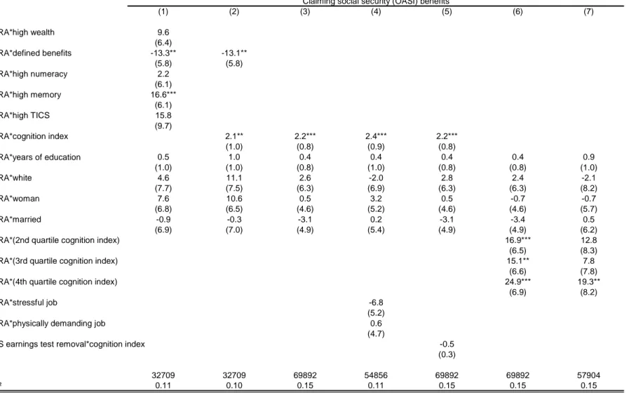
A limitation of model (5.1) is that it does not allow us to determine which of the many
interaction effects reported separately in table 5 are the most important. Interacting all 18
characteristics with the FRA indicator, the set of cohort dummies and the set of age dummies is
not feasible due to limited sample size and multicollinearity. A more parsimonious specification
introduces interactions with the most promising dimensions of heterogeneity, based on table 5:
pension characteristics, wealth, cognitive measures, and the basic socioeconomic variables. The
various specifications are given in table 6. Multicollinearity pushes the standard errors up, so that
few interaction terms remain significant. In column 1, where nine dimensions of heterogeneous
impact are considered simultaneously, the only significant effects are due to holding a defined
22
Benjamin, Brown, and Shapiro (2006) find that small-stakes risk aversion and short run discounting are less common among those with higher cognitive ability. These findings might conflict with our results, to the extent that non-standard preferences share a common component across domains.
24 benefit pension, and to high memory. The wealth effect shrinks somewhat, suggesting that it was
picking up in part the effect of cognitive ability. Combining the cognitive measures into a single
index confirms the positive impact of cognitive skills (column 2).23 Dropping the DB variable
(only available for a subsample of workers) does not significantly alter the results (column 3).
Of course, it may still be the case that these interaction effects are driven by unobserved
sources of heterogeneity. However, as noted above, a plausible causal interpretation of the DB
interaction effect is that the presence of a DB pension reduces the salience of the SS FRA, in
particular when the DB pension plan maintains a normal retirement age at 65. Accordingly, when
we restrict the sample to DB holders we find that the responsiveness to the SS FRA is lower for
those with a DB plan that has a normal retirement age at 65.24 By contrast, the negative impact of
low cognitive skills may seem harder to interpret causally. We first check that it is not capturing
the impact of stressful or otherwise demanding job characteristics (column 4), and that it is not
due to a lower sensitivity to the removal of the SS earnings test (column 5).25 Checking for non
linear effects, we find that most of the cognition effect is due to the lowest quartile, with smaller
differences among the upper three quartiles (column 6). Furthermore, the effect is weaker for
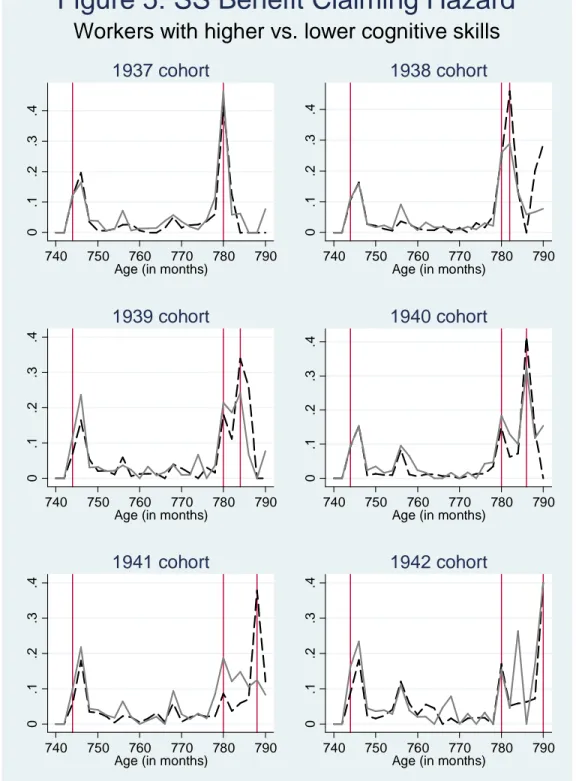
cohorts 1940+ compared to 1938-39 (column 7). This can be traced to the persistence of a large
age-65 spike for people with lower cognitive skills. As show by figure 5 (replicating figure 2 by
cognitive skill group), the age profiles of the hazard rate of claiming are very similar for people
with higher and lower cognitive skills born in 1937. Spikes at the new FRAs appear for cohorts
Their paper does not analyze reference dependence. Also, we do not find significant differences by levels of risk aversion.
23
See the Appendix for details on the cognition index.
24
The coefficient on FRA*(DB NRA=65) is -.095 (marginally significant with a standard error of.059).
25 born after 1938, but, for people with lower cognitive skills, the spike at the FRA is somewhat
smaller and the spike at age 65 persists. This suggests that people with lower cognitive skills
may be slower to learn about the change in the FRA and adapt it into their decision making.
Instead, they may use workers from earlier cohorts as a reference.2627
6. Implications of the results for framing Social Security reform
We interpret the empirical results presented above as suggesting that reference
dependence is a factor in claiming and retirement decisions. In this section, we introduce
reference dependence in a lifetime labor supply model in order to draw out its implications for
framing of Social Security reforms. Specifically, we derive conditions under which reference
dependence leads to a greater increase in employment in response to a benefit cut than would be
predicted by the wealth effect alone. The model echoes the way the SS administration frames
the retirement decision, as a tradeoff between income and “years to enjoy it”.
The set up is as simple as possible. Workers choose their optimal retirement and claiming
age (assumed to be the same for simplicity),28 by trading off years of leisure l against lifetime
consumption c. The age at death (T) is fixed and known, so choosing retirement age R is
25
Note that there is no significant difference across the two cognitive groups in the response to the removal of the SS earnings test.
26
This section has focused on claiming behavior, for which there is strong and robust evidence of responsiveness to the FRA. Analysis of employment exit and self-reported retirement indicates that there is little heterogeneity that can be detected in the FRA effect on these outcomes (results available from the authors).
27
Other explanations are possible. One would be that the two groups take the FRA as the claiming age recommended by the SSA, but only workers with higher cognitive skills read their statements and learn about the new FRA. We consider this explanation as less plausible given the care taken by the SSA not to imply any advice in their phrasing of the leisure / consumption tradeoff.
28
This assumption implies that we ignore the lower bound on claiming age. In the simulations described below, we account for it.
26 equivalent to choosing lifetime leisure: l =T−R(for convenience, we assume life begins at labor force entry). The budget constraint is: c=k+wR, where k+wR is a linear approximation
(in the vicinity of the FRA) of the lifetime income derived from retiring at age R; k (initial
wealth) and w (annual compensation, including the wage and the increment to the Social
Security benefit resulting from an additional year of work) are fixed parameters in this
approximation. This yields the standard static labor supply model, interpreted as a model of
lifetime labor supply:
). ( . . ) , ( max , l T w k c t s c l U l c − + = (6.1)
The SS rules and statements suggest a specific age, the FRA, as a reference. Let cFRA and
lFRA denote the levels of consumption and leisure from retiring and claiming at the FRA. Workers
may experience loss aversion with respect to either leisure or consumption or both: they may be
reluctant to reduce the number of “years to enjoy retirement” below the number implied by
retiring at their FRA, and they may be reluctant to consume less than the level implied by retiring
at the FRA. Following Tversky and Kahneman (1991), we incorporate reference dependence in a
two-good model with no uncertainty by specifying the payoff from choice (c,l) as:
), ( ) ( ) , (l c aR1 l R2 c UFRA = + (6.2) with FRA FRA FRA FRA l l if l u l u l R l l if l u l u l R > − = ≤ − = ) ( ) ( ) ( )) ( ) ( ( ) ( 1 1 1 λ and . ) ( ) ( ) ( )) ( ) ( ( ) ( 2 2 2 FRA FRA FRA FRA c c if c v c v c R c c if c v c v c R > − = ≤ − =λ 1
λ
andλ
2 are the coefficients of loss aversion, withλ
1,λ
2 >1 if there is loss aversion, and1 2 1=
λ
=27 0
>
a is an individual-specific parameter that allows for heterogeneity in the preference for
leisure.29
This specification captures an asymmetry in preferences with regard to losses and gains
around the FRA reference. Starting from the reference set by the FRA, the marginal utility of
increasing consumption by one dollar is v'(cFRA) whereas the utility loss from decreasing
consumption by one dollar is
λ
2v'(cFRA). Similarly, increasing leisure time by one day increases utility by au'(lFRA), whereas reducing it by one day decreases utility byaλ
1u'(lFRA). Both dimensions of loss aversion increase the likelihood that the FRA is the optimal retirement age.It is straightforward to show that the solution to problem 6.1 can be characterized by two critical
values of a: individuals with low preference for leisure (
) ( ' ) ( ' 1 FRA FRA l u c v w a
λ
< ) retire after the full
retirement age; those with high preference for leisure (
) ( ' ) ( ' 2 FRA FRA l u c v w
a> λ ) retire before the full retirement age; and workers with intermediate preferences for leisure
( ∈ ) ( ' ) ( ' ; ) ( ' ) ( ' 2 1 FRA FRA FRA FRA l u c v w l u c v w a
λ
λ
) retire exactly at the FRA. These three cases are illustrated infigure 6, which plots UFRA as a function of l, after substituting for consumption from the budget
constraint. UFRA has a kink at lFRA. This kink generates a mass point at the FRA in the distribution
of retirement ages. Let F denote the c.d.f. of a, and PFRA denote the fraction of workers retiring at
29
We introduce a as the only source of heterogeneity, and derive the distribution of retirement ages from the distribution of a. One could introduce other sources of heterogeneity, either in preferences –
1
λ
,λ
2, u(.) and v(.) may vary across individuals – or in budget constraints – variations in k, w or T. However, these other sources of heterogeneity have similar implications for the retirement age distribution: as long as they are continuously distributed (so that they do not generate a kink in28 the FRA. Then:
. ) ( ' ) ( ' ) ( ' ) ( ' 1 2 − = FRA FRA FRA FRA FRA l u c v w F l u c v w F P
λ
λ
(6.3)The fact that PFRA is strictly positive if
λ
1 >1 orλ
2 >1 shows that loss aversion in either of thetwo dimensions (loss of leisure or loss of benefits) is enough to generate the spike. However,
these two dimensions have opposite impacts on the rest of the retirement age distribution.
Starting from a situation without loss aversion (
λ
1 =λ
2 =1), an increase inλ
1 attracts workers who would otherwise work longer toward the FRA, thus reducing the average retirement age(see the model appendix for details). By contrast, an increase in
λ
2 attracts workers who wouldotherwise retire earlier toward the FRA, thus increasing the average retirement age. Overall, the
impact of reference dependence and loss aversion on the average retirement age is ambiguous a
priori.
Impact of the 1983 reform
The 1983 reform, as framed by the SSA, can easily be incorporated into the model as a
change in the reference age. In order to maintain the same level of benefits, workers born after
1937 must delay retirement by (FRA - 65 years). For instance, in order to receive 100% of the
primary insurance amount, workers born in 1937 must claim at age 65, whereas workers born in
1943 must delay claiming until age 66. In the model’s notation, the reform is such that ∆cFRA =0
and ∆lFRA <0. All other things equal, this has two effects on the retirement age distribution: First, the spike in the retirement hazard shifts to the new FRA. Second, the probability of retiring
29 before the FRA increases, whereas the probability of retiring after the FRA decreases. The
combined effect is an increase in the average retirement age. We now ask whether a different
framing of the reform would have yielded different results. Specifically, how does dE(R)/dk,
the response of the average retirement age R to a given shift in the intercept of the benefit
schedule dk, vary with the way the reform is framed? In all cases, we have
∫
− = − =T E l T l a f a da R E( ) ( ) *( ) ( ) , (6.4)where f is the density of a, and l*(a) is the level of leisure chosen by a worker given his
preference for leisure. The quantity we are interested in is
∫
− = f a da dk a dl dk R dE ) ( ) ( ) ( * . (7.5)The first framing option we consider is neutral: your benefit schedule is lower than the
schedule of your older peers, without reference to a specific age (see Figure 1). In this case the
response of *( )
a
l to the reform is simply given by differentiating the standard first order
conditions for an interior solution, yielding the standard wealth effect (see the model
appendix).30
Under the other two framing options, a reference point is explicitly given so that the
utility of a worker with preference for leisure a is described by equations 6.2 above, and
the optimal retirement age is characterized by solving the first order conditions for the cases in
which ) ( ' ) ( ' 1 FRA FRA l u c v w a
λ
< and ) ( ' ) ( ' 2 FRA FRA l u c v wa> λ ), and by setting l = lFRA if
hazard.
30
This only holds if there was no loss aversion and framing before the reform. Otherwise, it is unclear how a neutral framing of the reform would be perceived: would it cancel the initial reference? If
30 ∈ ) ( ' ) ( ' ; ) ( ' ) ( ' 2 1 FRA FRA FRA FRA l u c v w l u c v w a
λ
λ
. The two framing options differ by the fact that only the thirdframing option implies a change in the reference point.
In the second framing option, workers have the same reference point after the reform
(lFRA). However, SSA tells them that there is a cut in benefits for claiming at the FRA. In other
words, they still perceive that they meet a target if they retire at 65 after the reform, but the target
is now lower. This arises if the reform is framed as a change in the PIA (the benefit amount
available if claimed at the FRA) with no change in the FRA.
Finally, the third framing option is the one actually mandated by the reform: a change in
the FRA with no mention of a benefit cut. In this case, things remain as in the 2nd framing option
for workers with low and high preference for leisure. Things do however differ for workers with
intermediate preferences for leisure. The condition for claiming at the FRA is the same as under
the second framing option. However, the FRA itself changes, with 1 dk.
w dlFRA =
The model appendix shows that
2 3 ) ( ) ( > dk R dE dk R dE
, where the subscript indicates the
framing option. In the presence of reference dependence, the reform has a stronger impact if it is
framed as a change in the reference point than if it is framed as an equivalent change in the
benefit at the reference point. The comparison with
1 ) ( dk R dE
(neutral framing) is less
immediate; it depends on the parameters. However, empirical estimates suggest that
not, and if workers keep the initial reference point, the first framing option would be equivalent to the second option, described below.
31 1 3 ) ( ) ( > dk R dE dk R dE 31
. Indeed, Mastrobuoni (2009) finds that the average response to a 1 year
increase in the FRA (under the 3rd framing option, which is how it was framed by SSA) is a .5
year increase in the average retirement age. For workers at the FRA, loss aversion implies a 1 for
1 response. In this model, the .5 response must be a weighted average of 1 for people at the FRA
and δ (the average response for people above and below the FRA). This implies that δ <1. More precisely, the magnifying effect under the 3rd framing option is positively correlated with
the share of the population clustered at the FRA. Assuming that the response is roughly constant
for other workers, we have indeed
[
(1 )]
1[
( (1 )]
1 ) ( 3δ
δ
δ
+ =− + − − − ≈ FRA FRA FRA P w P P w dk R dE . (6.6)In sum, compared to a situation without a reference point (PFRA = 0), reference
dependence magnifies the impact of a reform if the reform is expressed as a change in the
reference point. This magnifying effect increases with the share of the population initially
clustered at the reference point. Figure 7 summarizes the main lesson of the model using
simulated data. We use CRRA specifications for u and v and assume that leisure preference a
follows a log-normal distribution with mean 1. We set w=1 and k=0, and simulate the model for
various values of the risk aversion coefficients in u and v and the variance of the log-normal
distribution. We select only those simulations that yield plausible distributions of the retirement
31
In our simulations discussed below,
1 ) ( dk R dE and 2 ) ( dk R dE
![[PDF] Formation générale pour programmer facilement avec le langage Java | Cours informatique](data:image/gif;base64,R0lGODlhAQABAIAAAP///wAAACH5BAEAAAAALAAAAAABAAEAAAICRAEAOw==)