Interstellar anatomy of the TeV gamma-ray peak in the IC443 supernova remnant★

(1)

HAL Id: hal-03037162

https://hal.archives-ouvertes.fr/hal-03037162

Submitted on 3 Dec 2020

HAL is a multi-disciplinary open access

archive for the deposit and dissemination of

sci-entific research documents, whether they are

pub-lished or not. The documents may come from

teaching and research institutions in France or

abroad, or from public or private research centers.

L’archive ouverte pluridisciplinaire HAL, est

destinée au dépôt et à la diffusion de documents

scientifiques de niveau recherche, publiés ou non,

émanant des établissements d’enseignement et de

recherche français ou étrangers, des laboratoires

publics ou privés.

IC443 supernova remnant�

P. Dell’ova, A. Gusdorf, M. Gerin, D. Riquelme, R. Güsten, A.

Noriega-Crespo, L. N. Tram, M. Houde, P. Guillard, A. Lehmann, et al.

To cite this version:

P. Dell’ova, A. Gusdorf, M. Gerin, D. Riquelme, R. Güsten, et al.. Interstellar anatomy of the

TeV gamma-ray peak in the IC443 supernova remnant�. Astronomy and Astrophysics - A&A, EDP

Sciences, 2020, 644, pp.A64. �10.1051/0004-6361/202038339�. �hal-03037162�

(2)

Astronomy

_&

Astrophysics

https://doi.org/10.1051/0004-6361/202038339

Interstellar anatomy of the TeV gamma-ray peak in the IC443

supernova remnant

?

P. Dell’Ova

1,2

_{, A. Gusdorf}

1,2

_{, M. Gerin}

2

_{, D. Riquelme}

3

_{, R. Güsten}

3

_{, A. Noriega-Crespo}

4

_{, L. N. Tram}

5,6

_{, M. Houde}

7

_,

P. Guillard

8

_{, A. Lehmann}

1,2

_{, P. Lesaffre}

1,2

_{, F. Louvet}

1,9

_{, A. Marcowith}

10

_{, and M. Padovani}

11

1_{Laboratoire de Physique de l’École Normale Supérieure, ENS, Université PSL, CNRS, Sorbonne Université, Université de Paris,}

75005 Paris, France

e-mail: pierre.dellova@ens.fr

2_{Observatoire de Paris, PSL University, Sorbonne Université, LERMA, 75014 Paris, France} 3_{Max-Planck-Institut für Radioastronomie (MPIfR), Auf dem Hügel 69, 53121 Bonn, Germany} 4_{Space Telescope Science Institute, 3700 San Martin Dr., Baltimore, MD 21218, USA}

5_{Stratospheric Observatory for Infrared Astronomy, Universities Space Research Association, NASA Ames Research Center,}

MS 232-11, Moffett Field, 94035 CA, USA

6_{University of Science and Technology of Hanoi, Vietnam Academy of Science and Technology, 18 Hoang Quoc Viet, Vietnam} 7_{Department of Physics and Astronomy, The University of Western Ontario, London, Ontario, N6A 3K7, Canada}

8_{Institut d’Astrophysique de Paris, CNRS UMR 7095, Sorbonne Université, 75014 Paris, France}

9_{AIM, CEA, CNRS, Université Paris-Saclay, Université Paris Diderot, Sorbonne Paris Cité, 91191 Gif-sur-Yvette, France}

10_{Laboratoire Univers et Particules de Montpellier (LUPM) Université Montpellier, CNRS/IN2P3, CC72, place Eugène Bataillon,}

34095, Montpellier Cedex 5, France

11_{INAF–Osservatorio Astrofisico di Arcetri, Largo E. Fermi 5, 50125 Firenze, Italy}

Received 4 May 2020 / Accepted 13 October 2020

ABSTRACT

Context. Supernova remnants (SNRs) represent a major feedback source from stars in the interstellar medium of galaxies. During the

latest stage of supernova explosions, shock waves produced by the initial blast modify the chemistry of gas and dust, inject kinetic energy into the surroundings, and may alter star formation characteristics. Simultaneously, γ-ray emission is generated by the interac-tion between the ambient medium and cosmic rays (CRs), including those accelerated in the early stages of the explosion.

Aims. We study the stellar and interstellar contents of IC443, an evolved shell-type SNR at a distance of 1.9 kpc with an estimated age

of 30 kyr. We aim to measure the mass of the gas and characterize the nature of infrared point sources within the extended G region, which corresponds to the peak of γ-ray emission detected by VERITAS and Fermi.

Methods. We performed 100_{× 10}0mapped observations of12CO,13CO J = 1–0, J = 2–1, and J = 3–2 pure rotational lines, as well as

C18_{O J = 1–0 and J = 2–1 obtained with the IRAM 30 m and APEX telescopes over the extent of the γ-ray peak to reveal the molecular}

structure of the region. We first compared our data with local thermodynamic equilibrium models. We estimated the optical depth of each line from the emission of the isotopologs13_{CO and C}18_{O. We used the population diagram and large velocity gradient assumption}

to measure the column density, mass, and kinetic temperature of the gas using12_{CO and}13_{CO lines. We used complementary data}

(stars, gas, and dust at multiple wavelengths) and infrared point source catalogs to search for protostar candidates.

Results. Our observations reveal four molecular structures: a shocked molecular clump associated with emission lines extending

between −31 and 16 km s−1_{, a quiescent, dark cloudlet associated with a line width of ∼2 km s}−1_{, a narrow ring-like structure associated}

with a line width of ∼1.5 km s−1_{, and a shocked knot. We measured a total mass of ∼230, ∼90, ∼210, and ∼4 M}

, respectively, for the

cloudlet, ring-like structure, shocked clump, and shocked knot. We measured a mass of ∼1100 Mthroughout the rest of the field of

observations where an ambient cloud is detected. We found 144 protostar candidates in the region.

Conclusions. Our results emphasize how the mass associated with the ring-like structure and the cloudlet cannot be overlooked when

quantifying the interaction of CRs with the dense local medium. Additionally, the presence of numerous possible protostars in the region might represent a fresh source of CRs, which must also be taken into account in the interpretation of γ-ray observations in this region.

Key words. ISM: supernova remnants – ISM: individual objects: IC443 – ISM: kinematics and dynamics – cosmic rays –

stars: formation

1. Introduction

The violent end of some stellar objects, a supernova (SN) explo-sion, is the beginning of an incredible sequence of energy injection in the surrounding interstellar medium (ISM). A SN

?_{The reduced datacubes are only available at the CDS via}

anony-mous ftp to cdsarc.u-strasbg.fr(130.79.128.5) or via http: //cdsarc.u-strasbg.fr/viz-bin/cat/J/A+A/644/A64

explosion ejects material with mass ranging from ∼1.4 to ∼20 M and a typical energy of 1050−52 erg (see, e.g.,Draine

2011) and drives fast shock waves about 104_{km s}−1_{ahead of the}

ejecta (the expelled stellar material) through the ISM. Already at early stages, SNe play a crucial, multifaceted role in the evolution of galaxies. The explosion and subsequent dispersion of matter is itself the most important source of elements heavier than nitro-gen in the gas phase (François et al. 2004). The fast shocks inject

(3)

kinetic energy that gradually decays in turbulence, which is a key process in the regulation of star formation on galactic scales (Mac Low & Klessen 2004). Fast shock fronts are also a rec-ognized site for the production of the bulk of cosmic rays, at least at gigaelectronvolt energies (CRs; see, e.g., Bykov et al. 2018;Tatischeff & Gabici 2018and references therein for recent reviews), although alternative origins are drawing more and more attention (such as superbubbles and Fermi bubbles; see, e.g.,Grenier et al. 2015;Gabici et al. 2019and references therein for recent reviews). Finally, the hot (106_–108 _{K) and relatively}

dense (1–10 cm−3_{) conditions in the ejecta could be favorable}

to the synthesis of cosmic dust up to hundred years after the explosion (see recent reviews byCherchneff 2014;Sarangi et al. 2018;Micelotta et al. 2018). After the first phases of expansion (free, then adiabatic), the temperature of the shock front drops to 106 _{K, allowing the gas to radiatively cool down. At this stage,}

the so-called supernova remnant (SNR) resembles a spherical shell of 10–20 pc radius, delimitated by regions in which shocks interact with the ambient medium.

This evolved SNR stage is also of fundamental importance to many aspects of galactic evolution. The fastest remaining shocks (between ∼30 and a few hundreds of kilometers per second) dis-sociate and ionize the pre- and post-shock medium and generate far-ultraviolet (FUV) photons (e.g.,Hollenbach & McKee 1989). More generally, shocks heat, accelerate, and compress the ambi-ent medium. They inject energy and trigger specific dust and gas-phase chemical processes (e.g.,van Dishoeck et al. 1993), hence significantly participating in the cycle of matter in galax-ies. Cosmic rays accelerated in the earlier stages of the explosion and trapped in the shock fronts now interact with the dense medium, producing observable X-ray to γ-ray photons (Gabici et al. 2009;Celli et al. 2019;Tang 2019and references therein). Cosmic rays of Galactic origin can also be reaccelerated in the shock regions (such as in W44, e.g.,Cardillo et al. 2016). Finally, evolved SNRs play a key role in star formation. Like all mas-sive stars, the progenitor of a SN explosion forms in a cluster in a dense and inhomogeneous environment, where lower-mass stellar companions have a greater life expectancy (Montmerle 1979). During its life on the main sequence, the progenitor drives stellar winds in the surrounding medium, possibly triggering a second generation of star formation in the neighboring molecu-lar clouds (e.g.,Koo et al. 2008). The compression and cooling caused by SNR shocks might also generate star formation (e.g.,

Herbst & Assousa 1977). In any case, the injection of energy exerted by SNRs in all possible forms (CRs, energetic photons, and shocks) likely alters locally the characteristics of all possible star formation events over significant spatial scales and times.

With the present study we aim to start characterizing as precisely as possible, and on fields as large as possible, the mechanisms of energy injection (shocks, photons, and CRs) exerted by an evolved SNR, and its effects on local star for-mation. Such a study must be performed on an evolved object, since energy injection effects can spread over the full dura-tion of the SNR phase, and are all the more visible when the SNR is old. In particular, we want to provide support for the study of CRs properties (acceleration, composition, and diffu-sion) in evolved SNRs. In these objects, CRs interact with the local medium through four processes that all generate γ-ray pho-tons: pion decay from the collision of hadronic CRs with the dense material, Bremsstrahlung from the interaction of leptonic CRs with the local dense medium, inverse Compton scattering of leptonic CRs with the local radiation field, and synchrotron emission of leptonic CRs gyrating around the local magnetic fields. Our first aim is to constrain the properties of the local

medium that is the target of these interactions: the mass and den-sity of all observed components, magnetic field structure, and radiation field structure.

Our second aim is to identify all possible sources of ongo-ing acceleration of “fresh” CRs additional to the “old” injection of CRs previously accelerated by the SNR. There can be two kinds of these sources: ionized regions in which kinetic energy is deposited and the magnetic field structure and ionization frac-tion make the accelerafrac-tion possible (such as [HII] regions; see

Padovani et al. 2019); or protostellar jets and outflows, where these conditions can be naturally combined. Our work can thus provide support for further studies of CR-related questions only if the study of local star formation is performed simultaneously. Indeed, Padovani et al. (2015, 2016) have shown that jets can accelerate low-energy CRs, which can be reaccelerated in the shock fronts of the remnant. Other studies have confirmed that supermassive star clusters neighboring SNRs can be a source of CRs (Hanabata et al. 2014). Conversely, an optimal charac-terization of CR action on the local formation is mandatory to better understand star formation in older galaxies. In fact, up to z ∼ 2 the star formation efficiency is higher (Madau & Dickinson 2014). The star formation regime observed in SNRs is reminis-cent of starburst galaxies, where SNe from a given generation of stars affect the next one.

The threefold and intertwined goals of our study (ISM, star formation, and CR) make the study of large fields mandatory. Cosmic ray studies rely on γ-ray spectra obtained with tele-scopes that only provide a limited spatial resolution, typically a few arcminutes. This extent is the minimum field for which we have to characterize the ISM and star formation as best as we can. This is why we have chosen to study a 100_{× 10}0_{field in the}

relatively evolved IC443 SNR (see Fig. 1). More particularly, with the present paper we investigate the physical conditions and dynamical structure of the molecular gas and its associa-tion with protostars in such a field located at the peak of γ-ray emission detected in the IC443 SNR, based on observations of the CO emission lines and its isotopologs. In Sect.2we present a summarized review of the source. In Sect.3, we present our observations and propose a description of the morphology and kinematics of the region, emphasizing three distinct molecular components. Section4focuses on the measure of the gas mass for these components. First we perform a local thermodynam-ical equilibrium (LTE) analysis of the 12_CO, 13_{CO, and C}18_O

emission lines and we build pixel-per-pixel, channel-per-channel population diagrams corrected for optical depth. Then we pro-pose a second method using a radiative transfer code based on the large velocity gradient (LVG) approximation. In Sect.5, we study the spectral energy distribution (SED) of point sources identified in infrared survey catalogs as well as the spatial dis-tribution of optical point sources detected with Gaia. Finally we summarize our findings in Sect.6.

Declination

[J2000]

γ-ray telescopes 50 IRAM 30m 12_CO(1_{− 0)} 22.500 50 1.5− 2.2 pc VLA 330 MHz

53

54

55

56

57

58

59

60 I

[MJy

· sr

− 1

]

Fig. 1.Spitzer/MIPS map (colors) of IC443 at 24 µm (Pinheiro Gonçalves et al. 2011;

Noriega-Crespo et al. 2009). In contours, the VLA emission map shows the mor-phology of the synchrotron emission at 330 MHz (Claussen et al. 1997). The white dot indicates the position of the PWN wind (Olbert et al. 2001b). The red box repre-sents one of the fields observed by Spitzer-IRS (Neufeld et al. 2004), corresponding roughly to the G region defined byHuang et al.(1986). The white box represents the 100_{× 10}0 _{field of our observations called}

“the extended G region”. The IRAM 30 m instrumental beam diameter corresponding to the12_{CO(1–0) transition and the size of}

the typical PSF of γ-ray telescopes (50_{) are}

indicated by white disks in the bottom left corner of the figure.

(Olbert et al. 2001a). The motion of the PWN is consistent with an age of 30 kyr for the SN event, and its detection strongly supports a core-collapse formation scenario for the SNR.

IC443 displays a shell morphology in radio, with two atomic sub-shells (shells A and B,Braun & Strom 1986). It is one of the most striking examples of a SNR interacting with neighboring molecular clouds. The most up-to-date and complete description of the structure and kinematics of both the atomic and dense molecular environment of the SNR was offered by Lee et al.

(2008, 2012). Their ∼1◦_{× 1}◦ _{map of the J = 1–0 transition of} 12_{CO allowed us to characterize both the incomplete}

molecu-lar shell interacting with shocks (toward the southern part of the SNR) and the molecular cloud that is associated with the remnant. Continuum radio emission in IC443 is partly corre-lated with the molecular shell and the secondary [HI] shell; see

Castelletti et al. (2011) for a detailed description of the low-frequency radio emission in IC443 at 74 and 330 MHz, and

Egron et al. (2017), Loru et al. (2019) for high and very-high frequency studies at 7 and 21.4 GHz, respectively.

CO emission was observed byDenoyer(1979a) toward the SNR, revealing three shocked CO clumps along the southern molecular ridge (labeled A, B, and C). Follow-up observations of CO J = 1–0 over a 500_{× 50}0_{field by}_{Huang et al.}₍₁₉₈₆_{) allowed}

the detection of new areas of shock-cloud interaction and to iden-tify five previously unknown CO clumps, extending the classifi-cation started byDenoyer(1979a) and providing the first mention of the G knot. The OH 1720 MHz line is a powerful diagnostic for the classification of SNRs interacting with molecular clouds

(Frail et al. 1996). Six masing spots were identified in IC443 byClaussen et al.(1997), all located in the G region delineated by Huang et al.(1986). The former authors proposed that OH masers spots could be promising candidates for the sites of CR acceleration.Lockett et al.(1999) improved the modeling of the shock origin for these maser lines, associated with moderate temperatures (50–125 K), local densities (∼105 _cm−3_{), and}

OH column densities on the order of 1016 _cm−2_{, then} _Wardle

(1999) added the effect of the dissociation of molecules by FUV photons in molecular clouds subject to CR and X-ray ionization (see Hoffman et al. 2003, Hewitt et al. 2006, 2008, 2009

for recent studies). From J = 1–0 12_{CO and HCO}+ _emission,

Dickman et al.(1992) measured a mass of 41.6 Mfor “clump

G”, and estimated that a total molecular mass of 500–2000 M

is interacting with the SNR shocks, which corresponds to 5–10% of the SN energy considering that the average velocity of the clumps is 25 km s−1_._{Zhang et al.}₍₂₀₁₀_{) showed that two distinct}

structures are resolved in region G, labeling G1 the strongest

13_{CO peak and G2 the previously mentioned shocked clump.}

Lee et al.(2012) measured a mass of 57.7 ± 0.9 Mfor the clump

G2. Oddly,Xu et al.(2011) measured a mass of 2.06 × 103 _M

for “cloud G”, which is much higher than the previous estimates. Several molecular shocks were mapped within the SNR using

12_{CO lines (e.g.,}_{White et al. 1987}_,_{Wang & Scoville 1992} _for

clumps A, B, and C). In particular, the kinematics of clump G were characterized in detail byvan Dishoeck et al.(1993), who presented observations of the rotational transition J = 3–2 of CO along the shocked molecular ring at a spatial resolution of

(5)

2000_–3000_{. In the last 10 yr, the large-scale molecular contents}

of IC443 have been scrutinized with increasing precision and completeness, since several authors have mapped the J = 1–0 transition of the isotopologs 12_CO, 13_{CO, and C}18 _{over large}

fields (from 400_{× 45}0_{to 1.5}◦_{× 1.5}◦_;_{Zhang et al. 2010}_,_{Lee et al.}

2012, Su et al. 2014). Several submillimeter observations of IC443 were performed to characterize the shocked molecular gas (e.g., van Dishoeck et al. 1993 for a study of the shock chemistry in the southern ridge toward the clumps B, C, and G). Notably, the ground state of shocked ortho-H2O was detected

toward the clumps B, C, and G (Snell et al. 2005).

The incomplete shell-morphology is also observed in the J, H, K bands observed by 2MASS (Two-Micron All-Sky Sur-vey; Rho et al. 2001), as well as in infrared and far-infrared observations by Spitzer-MIPS (Pinheiro Gonçalves et al. 2011;

Noriega-Crespo et al. 2009) and the Wide-field Infrared Sur-vey Explorer (WISE;Wright et al. 2010). Excitation by shocks was suggested as the most likely scenario for the emission lines detected in IR, instead of X-ray or FUV mechanisms (e.g., [OI],Burton et al. 1990).Rho et al. (2001) analyzed the emission of [OI] with shock models, suggesting a fast J-type shock (∼100 km s−1_{) in the NE atomic shell, and a C shock}

(vs=∼30 km s−1) propagating in the southern molecular ridge.

In an effort to study molecular shocks, H2pure rotational

transi-tions were mapped toward clump G by ISOCAM (ISO;Cesarsky et al. 1999) and compared to non-stationary shock models, as well as toward clumps C and G by Spitzer-IRS (Infrared Spectro-graph;Neufeld et al. 2007). Molecular clumps B, C, and G were also observed by Akari (Shinn et al. 2011) and by the Strato-spheric Observatory for Infrared Astronomy (SOFIA; Reach et al. 2019). All these studies were carried out in small fields (∼10_{× 1}0_{) and allowed to put constraints on the shock velocity}

(∼30 km s−1_{) and pre-shock density (∼10}4_cm−3_{), and to outline}

similarities with protostellar shocks in the southern ridge where we aim to focus on the extended G region.

The optical emission is well correlated with radio and [HI] features, reproducing shells A and B. In particular, the SNR displays bright, filamentary structures toward the northeastern part of the remnant (Fesen & Kirshner 1980;Alarie & Drissen 2019). IC443 was fully mapped by the Sloan Digital Sky Survey (SDSS;York et al. 2000). There are no bright features toward the extended G region, but optical studies offered constraints on the global characteristics of IC443.Ambrocio-Cruz et al.(2017) estimated an age of ∼30 kyr and an energy of 7.2 × 1051_erg

injected in the environment by the SNR from the comparison of observations of [Hα] with SNR models (Chevalier 1974).

The shell-like structure of IC443 in radio, centrally filled in X-rays, puts the remnant into the category of mixed-morphology SNRs (Petre et al. 1988; Rho & Petre 1998). Observations of the hard X-ray contents of IC443 (up to 100 keV) by BeppoSAX show hints of shock-cloud interaction (Bocchino & Bykov 2000). The X-ray Multi-Mirror mission (XMM-Newton) mapped IC443 in the ranges 0.3–0.5 and 1.4–5.0 keV with an unprecedented field of view and spatial resolution (Bocchino & Bykov 2003), and showed that the soft X-ray emission is partly absorbed by the nearby molecular cloud (Troja et al. 2006).Troja et al. (2008) reported the detection of a ring-shaped ejecta encircling the PWN, associated with a hot metal rich plasma for which the abundances are in agreement with a core-collapse scenario.

The CR content and γ-ray emission in IC443 have been scrutinized by multiple observatories. Fermi-LAT (Large Area Telescope) detected an extended γ-ray source in the 200 MeV– 50 GeV energy band (Ackermann et al. 2013).Abdo et al. 2010

showed that the spectrum is well reproduced by the decay of

neutral pions and pinpointed the clouds B, C, D, F, and G as targets of interaction.Tavani et al.(2010) reported the detection of γ-ray enhancement toward the NE shell in the 100 MeV– 50 GeV range observed by AGILE (Astro-Rivelatore Gamma a Immagini Leggero). In their hadronic model, cloud “E” is the suggested target for interaction with CRs. Interestingly, the loca-tion of the γ-ray peak differs between the lower energy detecloca-tions by Fermi and the Energetic Gamma Ray Experiment Telescope (EGRET,Esposito et al. 1996) and the very high energy detec-tions by the Major Atmospheric Gamma-ray Imaging Cherenkov Telescope (MAGIC) and the Very Energetic Radiation Imaging Telescope Array System (VERITAS, Albert et al. 2007). This tendency is also verified byTavani et al.(2010) who located the 100 MeV γ-ray peak close to the Fermi/EGRET position and further toward NE. Recently, VERITAS Collaboration (2015) presented an updated Fermi map where the position of the peak was shifted and consistent with VERITAS, exposing the uncer-tainty on the localization of the peak from the analysis of γ-ray observations. The choice of the region studied in this paper is based on the teraelectronvolt γ-ray significance map from

VERITAS Collaboration(2015), which emphasizes the extended G region as a favorable target of high-energy CR interaction with dense molecular gas.

Explicit magnetic field studies toward IC443 are scarce.

Wood et al.(1991) performed 6.1 cm polarimetric observations of the northeast rim of IC443. These authors found that the local magnetic field is rather correlated with the rim structure, but with no clear orientation (i.e., parallel or perpendicular) to it. OnlyHezareh et al.(2013) conducted a polarization study toward clump G. These authors observed circular and linear polarization of the CO (1–0) and (2–1) lines with the Institut de Radioas-tronomie Millimétrique 30 m antenna (hereafter IRAM 30 m), and linear polarization maps from the dust continuum with the Acatama Pathfinder EXperiment (hereafter APEX). Their study constituted a crucial step toward the characterization of the inter-action of CRs with the magnetic field in the extended G region.

Star formation in IC443 was the focus of a few studies, but early investigations lacked sufficient data to make clear find-ings. Recently,Xu et al.(2011) used color criteria for the point sources detected by the Infrared Astronomical Satellite (IRAS) and 2MASS to identify protostellar objects and young stellar object (YSO) candidates and showed their association to sev-eral regions of the SNR interacting with neighboring molecular structures, including clump G. Su et al. (2014) confirmed the shell structure of the distribution of YSO candidates using a selection method based on color-color diagrams inferred from WISE bands 1, 2, and 3 and 2MASS band K. Both studies con-cluded that the formation of this YSO population is likely to have been triggered by the stellar winds of the progenitor.

3. Observations, reduction, and dataset

3.1. Observations 3.1.1. APEX

A mosaic of the IC443G extended region was carried out with APEX1_{. The APEX observations toward IC443G were} conducted on September 11, 2018. The heterodyne receivers

1 _{This publication is partly based on data acquired under project}

M9508A_102 with the Atacama Pathfinder EXperiment (APEX). APEX is a collaboration between the Max-Planck-Institut für Radioas-tronomie (MPIfR), the European Southern Observatory, and the Onsala Space Observatory.

(6)

Table 1. Spectroscopic parameters corresponding to the observed lines. Specie Jup νi j(GHz) Ai j(s−1) gup Eup(K) 12_CO ₁ _115.2712018 _{7.203 × 10}−8 ₃ _5.53 12_CO ₂ _{230.5380000 6.910 × 10}−7 ₅ _16.6 12_CO ₃ _{345.7959899 2.497 × 10}−6 ₇ _33.19 13_CO ₁ _110.2013543 _{6.294 × 10}−8 ₃ _5.29 13_CO ₂ _220.3986841 _{6.038 × 10}−7 ₅ _15.87 13_CO ₃ _330.5879652 _{2.181 × 10}−6 ₇ _31.73 C18_O ₁ _109.7821734 _{6.266 × 10}−8 ₃ _5.27 C18_O ₂ _219.5603541 _{6.011 × 10}−7 ₅ _15.81

Notes. The quantity Jup is the rotational quantum number, νi jand Ai j

are the frequency and Einsten coefficient of the pure rotational transi-tion, respectively (3 = 0, where v is the vibrational quantum number). The quantities Eupand gupare the energy and degeneracy

correspond-ing to the upper level, respectively. The values given are taken from the Cologne Database for Molecular Spectroscopy (Müller et al. 2001,

2005; Endres et al. 2016) and Jet Propulsion Laboratory database (Pickett et al. 1998) and are the numeric values used for all our measures.

PI230 and FLASH345 (First Light APEX Submillimeter Het-erodyne receiver; Heyminck et al. 2006), operating at 230 and 345 GHz, respectively, were used in combination with the FFTS4G and the Max-Planck-Institut für Radioastronomie (MPIfR) fast Fourier transform spectrometer backend (XFFTS;

Klein et al. 2012). This setup allowed us to cover a total field of 100_{× 10}0 _{toward the center of the molecular region G. The}

observations were performed in position-switching and on-the-fly mode using APECS software (Muders et al. 2006). Table1

contains the spectroscopic parameters of the observed lines and Table2contains the corresponding observing setups2_.

The central position of all observations was α[J2000]= 6h16m37.5s, δ[J2000]= +22◦3500000. The off-position

used was α[J2000]= 6h17m35.8s, δ[J2000]= +22◦3300800, in the

inner region of the SNR. We checked the focus during the observing session on the stars IK Tau and R Dor. We checked line and continuum pointing every hour locally on V370 Aur, Y Tau, IK Tau, and R Dor. The pointing accuracy was better than ∼300 _{rms, regardless of which receiver we used. The}

absolute flux density scale was also calibrated on these sources. The absolute flux calibration uncertainty was estimated to be ≈15% during our observations. We used the GILDAS3 _package to calibrate and merge the data of all subfields to produce a mosaic, and extract the spectral bands containing the signal corresponding to the (2–1) rotational transitions of12_CO,13_CO,

C18_{O, and the (3–2) rotational transitions of} 12_{CO and} 13_CO.

The reduction included first order baseline subtraction, spatial, and spectral regridding. The final products of this reduction process are spectral cubes centered on the previously cited rotational lines with a resolution of 0.5 km s−1 _{to increase the}

signal-to-noise ratio (S/N), which is more than enough for the

2 _{APEX telescope efficiencies are taken from} _http://www.

apex-telescope.org/telescope/efficiency/index.php,

and IRAM telescope efficiencies are taken from https://www. iram-institute.org/medias/uploads/eb2013-v8.2.pdf

3 _{The Grenoble Image and Line Data Analysis Software is developed}

and maintained by IRAM to reduce and analyze data obtained with the 30 m telescope and Plateau de Bure interferometer. Seewww.iram.fr/ IRAMFR/GILDAS

expected line widths (nominal spectral resolutions are indicated in Table 2). The observed area is shown in the white box in Fig.1.

3.1.2. IRAM 30 m

The same mosaic of the IC443G extended region was carried out with the IRAM 30 m4_{. The IRAM observations toward} IC443G were conducted during one week, from February 20, 2019 to February 24, 2019. The heterodyne receiver Eight MIxer Receiver (EMIR; Carter et al. 2012), operating at 115 and 230 GHz simultaneously, was used in combination with the FTS200 and Versatile SPectrometer Array (VESPA) back-ends. This setup allowed us to cover the same total field of 100_{× 10}0 _{toward IC443. The observations were performed in}

position-switching and on-the-fly mode. Table 2 contains the corresponding observing setups.

The central position of all observations was the same as that used for APEX observations, α[J2000]= 6h16m37.5s,

δ[J2000]= +22◦3500000. The off-position used was α[J2000] =

6h₁₇m₅₄s_{, δ}_[J2000]_{= +22}◦₄₇0₄₀00 _{in the northeastern ionized}

region of the SNR. We checked the continuum pointing and focus every hour during the observing sessions on several bright stars. The pointing accuracy was better than ∼300_{rms. The}

abso-lute flux calibration uncertainty was estimated to be ≈15%. We also used the GILDAS package to calibrate and merge the data of all subfields to produce a mosaic, and extract the spectral bands containing the signal corresponding to the (1–0) rotational tran-sitions of12_CO,13_{CO, C}18_{O, and (2–1) rotational transition of} 12_{CO. The reduction process and final products are identical to}

what was presented in the previous subsection. The observed area is shown in the white box in Fig.1.

3.1.3. Comparison between the IRAM 30 m and APEX telescope data cubes

We estimated the systematic errors between the IRAM 30 m and APEX based on the data cubes corresponding to the observation of the rotational transition12_{CO(2–1) by both telescopes. For a}

visual comparison of the two data cubes, the channel maps are given in Figs.2(IRAM 30 m) andD.3(APEX). We found no evi-dence of systematic pointing error between the two data cubes. We also performed a quantitative comparison of the two spec-tral cubes. First, we resampled the data cubes to get the same spatial and spectral resolution. The spatial resolution was set to the nominal resolution of APEX θ = 28.700_{, and the spectral}

res-olution was set to the nominal resres-olution of the IRAM 30 M ∆3 =0.5 km s−1. Then, in each frequency channel and every sin-gle pixel of the mosaic we compared the signal detected by the two telescopes, for which the signal is greater than 3σ. The results of this complete investigation are represented on a TAPEX

mb

vs. T30 m

mb 2D histogram shown in Fig. 3. We determined the

best linear fit x 7→ a · x + b corresponding to the data disper-sion between the two telescopes. The parameters given by the χ2

minimization are a = 0.88; b = −0.35, indicating a slight over-estimate in the measurement of the flux by the IRAM 30 m with respect to APEX measurements, at least in the scope of our observations. Thus, our measurements are characterized by a systematic error of approximately 12%. This could be due

4 _{This work is based on observations out under project number 169-18}

with the IRAM 30 m telescope. IRAM is supported by INSU/CNRS (France), MPG (Germany) and IGN (Spain).

(7)

Table 2. Observed lines and corresponding telescope parameters for the observations of the extended G region of IC443.

Species 12_CO 12_CO 12_CO 12_CO 13_CO 13_CO 13_CO _C18_O _C18_O

Line (1–0) (2–1) (2–1) (3–2) (1–0) (2–1) (3–2) (1–0) (2–1)

Telescope IRAM 30 m IRAM 30 m APEX APEX IRAM 30 m APEX APEX IRAM 30 m APEX ν(GHz) 115.271 230.538 230.538 345.796 110.201 220.399 330.588 109.782 219.560

FWHM (00₎ _22.5 _11.2 _28.7 _19.2 _23.5 _30.1 _20.0 _23.6 _30.2

Sampling (00₎ _3.5 _3.5 ₆ ₆ _3.5 ₆ ₆ _3.5 ₆

Receiver EMIR EMIR PI230 FLASH345 EMIR PI230 FLASH345 EMIR PI230

Obs. dates 19-02-20 19-02-20 18-09-11 18-09-11 19-02-20 18-09-11 18-09-11 19-02-20 18-09-11 19-02-24 19-02-24 18-09-11 18-09-11 19-02-24 18-09-11 18-09-11 19-02-24 18-09-11 Feff 0.94 0.92 0.95 0.95 0.91 0.95 0.95 0.94 0.95 Beff 0.78 0.59 0.73 0.63 0.51 0.73 0.63 0.78 0.73 Tsys(K) 172 321 146 291 118 129 330 118 129 ∆3(km s−1) 0.5 0.5 0.1 0.1 0.5 0.1 0.1 0.5 0.1 rms (K) 0.035 0.039 0.069 0.066 0.025 0.084 0.080 0.022 0.130

Notes. ν is the frequency of the transition, FWHM corresponds to the full width at half maximum of the instrumental beam, Feff is the forward

efficiency, and Beffthe beam efficiency of the dish. The quantity Tsysis the average system noise temperature and ∆3 the nominal spectral resolution.

PWV is the precipitable water vapor, and rms is the standard deviation measured on the baseline resampled with a spectral resolution of 0.5 km s−1

to allow direct comparison between the data from the IRAM 30 m and APEX telescopes.

to inaccurate correction of telescope efficiencies and/or abso-lute flux calibration. Also, according to the dispersion around the instrumental linear model, our measurements are affected by a random error characterized by a standard deviation of 305 mK.

3.2. Morphology of the region

Our 100_{× 10}0_{, ∼10–30}00 _{resolution maps of}12_{CO and}13_{CO in}

the extended G region provide a detailed picture of the mor-phology of molecular clumps. Figure 4 (left panel) shows the emission in12_{CO(2–1) integrated between 3 = −40.0 km s}−1_and

3 = +30 km s−1_{mapped with the IRAM 30 m. This wide}

inter-val of velocity includes all the components of the signal that are detected within the bandpass of our observations toward the extended G region. This map reveals a structured region with two main molecular structures that are spatially separated. The first structure (bottom center in Fig.4) has a peak integrated inten-sity of 578 K km s−1_{, which is a magnitude higher than the peak}

integrated intensity of the second structure (top right in Fig.4) that is around 63 K km s−1_.

Figure2shows the channel maps corresponding to the IRAM 30 m observations of the12_{CO J = 2–1 transition, which gives}

the finest spatial resolution of all our observations: θ = 11.200_{, or}

∼0.1 pc at the adopted distance of 1.9 kpc. The channel maps cor-responding to other transitions of12_{CO and its isotopolog}13_CO

are also available in the appendix:

– 12_{CO(1–0) mapped with the IRAM 30 m (Fig.}_D.1_);

– 13_{CO(1–0) mapped with the IRAM 30 m (Fig.}_D.2_);

– 12_{CO(2–1) mapped with APEX (Fig.}_D.3_);

– 12_{CO(3–2) mapped with APEX (Fig.}_D.4_).

Several faint and sparse knots are detected over all the field of observations, especially around the systemic velocity of IC443 3LSR=−4.5 km s−1(Hewitt et al. 2006). These structures,

notice-able between 3 = −7.5 km s−1_{and 3 = −1.5 km s}−1_{, might either}

correspond to a slice of turbulent medium driven by the SN shockwave and/or belong to the ambient gas associated with the NW-SE molecular cloud in which IC443G is embedded

(Lee et al. 2012). Other than that, the description of the region probed by our observations can be divided into the following six distinct structures:

1. Cloudlet: in the upper part of the field we observe a large (∼50_{× 2}0_{, i.e., ∼2.8 × 1.1 pc) elongated cloudlet detected}

between 3 = −7.0 km s−1 _{and 3 = −5.5 km s}−1 _{(indicated by the}

letter “A” in Fig.2), which is also detected in12_{CO(3–2). This}

structure was labeled G1 byZhang et al.(2010), as part of the double-peaked morphology of the extended G region. The13_CO

J = 1–0 counterpart of this structure is much brighter than the other main structures in the field, and it is also detected in the transitions J = 2–1 and J = 3–2, and in C18_{O J = 1–0 and J = 2–1.}

This structure was also presented and characterized byLee et al.

(2012) who proposed the label SC 03, among a total of 12 SCs (of size ∼10_{) found in IC443.}

2. Ring-like structure: a ring-like structure seemingly lying in the center of the field (indicated by the letter “B” in Fig.2), appearing between 3 = −5.5 km s−1_{and 3 = −4.5 km s}−1_{and also}

detected in12_{CO(3–2). It has a semimajor axis of 1.5}0_{, or 0.8 pc.}

This structure might be spurious and is likely to be physically connected to the elongated cloudlet as both are spatially contigu-ous and their emission lines are spectrally close. It is partially detected as well in our observations of 13_{CO J = 1–0, J = 2–1}

and J = 3–2, and also has a faint, partial counterpart in C18_O

J = 1–0 and J = 2–1. To understand the nature of this region we searched for counterparts in Spitzer Multiband Imaging Pho-tometer (MIPS), WISE, DSS and XMM-Newton data; and in near-infrared and optical point source catalogs (Sect.5), without success. Owing to projection effects, this apparent circular shape could also be explained by an unresolved and clumpy distribution of gas.

3. Shocked clump: in the lower part of the field we iden-tify a very bright clump emitting between 3 = −31.0 km s−1_and

3 =16 km s−1. This structure of size ∼20_{× 0.75}0(∼1.1 × 0.4 pc), which is detected in the12_{CO(3–2) transition as well, belongs to}

the southwestern ridge of the molecular shell of the SNR and has been described as a shocked molecular structure by sev-eral studies (van Dishoeck et al. 1993; Cesarsky et al. 1999;

(8)

22◦400 350 300 0 5 10 15 20 22◦400 350 300 0 5 10 15 20 22◦400 350 300 0 5 10 15 6h17m00s 16m30s 22◦400 350 300

Right Ascension [J2000]

Declination

[J2000]

6h17m00s 16m30s6h17m00s 16m30s6h17m00s 16m30s 0 2 4 6 8

T

m

b

[K]

Fig. 2.Channel maps of the12_{CO(2–1) observations carried out with the IRAM 30 m telescope. Each panel represents the emission integrated over}

an interval of velocity along the line of sight. Velocity intervals are indicated on the top left corner of each panel. Velocity channels represented in this figure are between 3 = −24 km s−1_{and 3 = +12 km s}−1_{, covering all the spectral features detected toward the extended G region. Structures}

described in Sect.3.2are indicated with the corresponding letters.

Snell et al. 2005;Shinn et al. 2011;Zhang et al. 2010). The core of the shocked clump (indicated by the letter “C” in Fig.2) is also detected in13_{CO in the transitions J = 1–0, J = 2–1, and J = 3–2,}

and in C18_{O J = 1–0 and J = 2–1.}

4. Shocked knot: an additional shocked knot (indicated by the letter “D” in Fig.2) is also detected to the west of the previously described structure. This fainter and smaller structure is spatially separated from the main shocked clump.

5. At the same position as the shocked clump and extending southward and westward, we find a faint, elongated clump emit-ting between 3 = 5.0 km s−1 _{and 3 = 7.5 km s}−1_{. This structure}

(indicated by the symbol “*” in Fig.2) spatially coincides with the shocked clump, yet the peak velocity is not exactly the same (see developments on kinematics of the region in Sect.3.3). It has a faint counterpart in13_{CO(1–0). Observations of the}

ambi-ent molecular cloud byLee et al.(2012) indicate this structure as part of a faint NE-SW complex of molecular gas in the velocity range +3 km s−1_{< 3}_LSR_{< +10 km s}−1_.

6. Finally, the 13_{CO(1–0) map (Fig.} ₄_{, right panel and}

Fig. D.2) indicates a large clump of gas extending from the bottom center to the right end of the field, with a bright knot in the bottom right corner of the field. However, this structure has no bright, well-defined counterpart in any of the12_{CO transitions}

maps. It is spatially and kinematically correlated with the faint and diffuse12_{CO J = 1–0 and J = 2–1 emission seen in the}

veloc-ity range −5.5 km s−1_{< 3}_LSR_<_{−2 km s}−1_{. From the comparison}

with the12_{CO observations of}_{Lee et al.}₍₂₀₁₂_{) and}13_CO

obser-vations ofSu et al.(2014) toward the SNR, we conclude that this structure is part of the western molecular complex observed in the velocity range −10 km s−1_{< 3}_LSR_<_{0 km s}−1_.

3.3. Kinematics of the region

Using the nominal spectral resolution of 0.5 km s−1 _attained

with our IRAM 30 m12_{CO J = 2–1 observations, we identified}

(9)

5 15 25 T30m mb [K] 5 10 15 20 25 30 T APEX mb [K] 100 101 102 103 bin coun ts

Fig. 3. Two-dimensional histogram of TAPEX

mb vs. Tmb30m 2D

represent-ing the complete comparison between the data cubes obtained with the IRAM 30 m and APEX telescopes observations of the transition

12_{CO(2–1) in the extended G region. The two cubes were resampled to}

the same spatial and spectral resolution. Every spectral channel in every single pixel is compared and shown in the histogram. The dashed black line represents the 1:1 relation expected between the two spectral cubes if the data was identical. The solid black line represents the empirical relation that is measured by determining the best linear fit correspond-ing to the data dispersion, uscorrespond-ing a threshold of 1.5 K to best describe the high signal-to-noise bins.

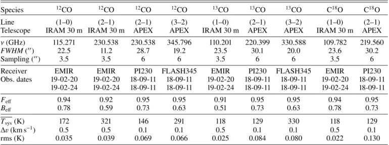
based on the determination of the first and second moment maps (Fig.5, left and center) of the12_{CO(2–1) data cube. We also}

pro-duced the moments maps of the12_{CO(3–2) data cube toward the}

ring-like structure (Fig. 5, right) to profit from the spectral resolution of 0.1 km s−1_.

1. The cloudlet has a mean velocity of about 3LSR=

−5.5 km s−1_{that is remarkably uniform throughout the structure.}

We measured 3LSR=−5.7 ± 0.3 km s−1from the centroid of the 13_{CO lines, contrasting with the velocity of IC443 in the local}

standard of rest by more than 1 km s−1_{. It is likely that this}

dis-crepancy is due to a distinct velocity component with respect to the rest of the molecular gas in the extended G region. If this is not the case, this velocity shift could correspond to a maximum displacement of the kinematic distance ∆d ≈ 300 pc (follow-ing Wenger et al. 2018). Yet, the velocity wings of the 12_CO

lines are still within the velocity range of the maser source in IC443G. The second moment map reveals a much lower veloc-ity dispersion within the cloudet than for the shocked clump. It varies between ∼5 and ∼7 km s−1_{, which is slightly higher}

than the velocity dispersion across the background field, around ∼4 km s−1_.

2. The apparent ring-like structure is further analyzed in the two right panels of Fig. 5, where the first and second moment maps are determined for the12_{CO(3–2) data cube obtained with}

APEX. The superior spectral resolution of the APEX data cube offers a better precision in the determination of the moment maps, at the cost of a lower spatial resolution. In the first moment map the mean velocity gradient within the ring sug-gests that the structure is rotating or expanding isotropically, as the mean velocity field varies between 3LSR=−4.7 km s−1 and 3LSR=−5.8 km s−1 from the western to the eastern arc of the

ring. This apparent velocity gradient could be also due to system-atic velocity variations between two or more distinct sub-clumps that are not well resolved by our J = 3–2 observations (θ = 19.200_,

∼0.2 pc). The velocity dispersion measured within the ring-like structure varies between 1 and 3 km s−1_{, with a positive gradient}

from the eastern part to the western part of the structure where it spatially connects to the cloudlet.

3. The shocked clump has a mean velocity varying between 3LSR=−6 km s−1 and 3LSR=−8.5 km s−1 throughout its struc-ture. We caution that these mean velocities are uncertain because the self-absorption and asymmetric wings characterizing the line emissions of12_{CO might bias the value of the centroid. In fact,}

careful measurement of the centroid of13_{CO lines using a single}

Gaussian function favors a velocity centroid of −4.4 ± 0.2 km s−1

for the shocked clump, which is consistent with the velocity vLSR=−4.5 km s−1of the maser in IC443G (Hewitt et al. 2006).

The second moment map represents important velocity disper-sions, spanning from ∼15 and up to ∼36 km s−1 _{within the}

shocked gas, increasing toward the center of the clump.

4. The shocked knot has a mean velocity v = −9 km s−1_that

is slightly shifted with respect to the shocked clump. The second moment map shows a uniform velocity dispersion of ∼25 km s−1_,

similar to the dispersion measured within the main shocked molecular structure.

The rest of the field of observation has a quasi-uniform mean velocity of ∼−4.1 to ∼−2.8 km s−1_{, which is slightly different}

than the mean velocity of IC443G in the local standard of rest but consistent with the ambient NW-SE molecular cloud in which IC443G is embedded (Lee et al. 2012). The velocity dispersion of this ambient gas spans from <1 to ∼10 km s−1_{in a few areas}

where the velocity dispersion is locally enhanced, with an aver-age of ∼4 km s−1_{. Excluding the contribution of the shocked}

structures and localized high-velocity dispersion knots, velocity dispersions measured from the12_{CO J = 2–1 line in the extended}

G field span a range of rms velocity σv=0.4–1.3 km s−1 in the

ambient gas, and σv=1.2 to 1.8 km s−1toward the cloudlet. At a

temperature of 10 K, the thermal contribution is σv=0.32 km s−1

and it is likely that small-scale motions within the complex of molecular gas contribute to the measured dispersion, hence the ambient cloud is mostly quiescent, with turbulent motions smaller than 1 km s−1_{. The velocity dispersion measured toward}

the cloudlet with the13_{CO lines is σ}

v=0.8 ± 0.1 km s−1, which is

consistent with typical molecular condensations (Larson 1981). Thus, we do not find any kinematic signature of interaction of the cloudlet nor the ambient cloud with the SNR shocks in the extended G region, except for the few localized high-velocity dispersion knots.

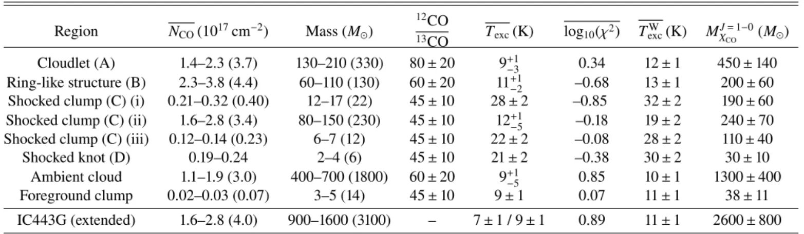
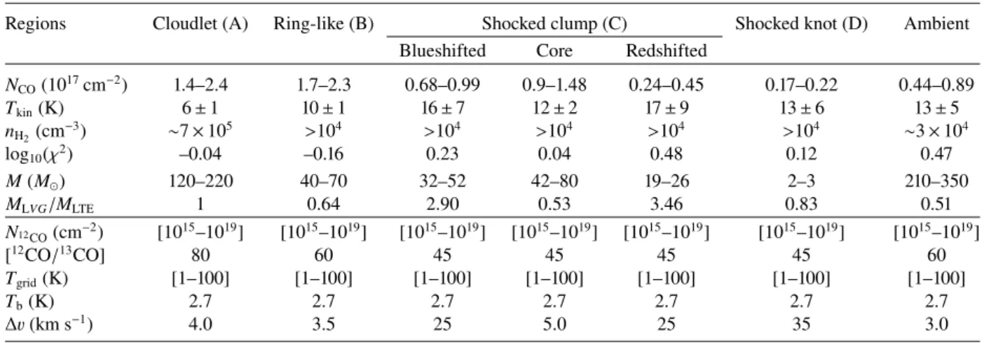
4. Column density and mass measurements

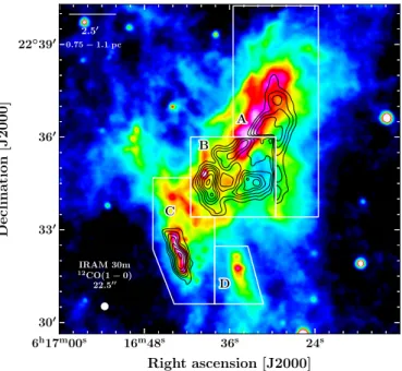
4.1. Spatial separation of spectrally uniform structures We aim to measure the mass associated with each molecular structures described in the previous section. We defined spatial boundaries enclosing these structures and independently studied the spectral data corresponding to each subregion of the field. The spatial boxes defined for the cloudlet (A), ring-like struc-ture (B), shocked clump (C), and shocked knot (D) are shown in Fig.6, and the average spectra obtained in these boxes are presented in Figs.8 and7 for every line from CO and its iso-topologs, which are available in our IRAM 30 m and APEX data cubes. The choice of the boundaries is based on our morpho-logical classification, but we carefully checked that the brightest

(10)

6h₁₆m₅₀s ₄₀s ₃₀s ₂₀s 22◦380 360 340 320

Right Ascension [J2000]

Declination

[J2000]

1 pc 101 102 R T m b d v [K · km · s − 1] 6h₁₇m₀₀s ₁₆m₄₈s ₃₆s ₂₄s 22◦₃₉0 360 330 300 Right Ascension [J2000] Declination [J2000]

Fig. 4.Left: 0th moment of the12_{CO(2–1) observations carried out with the IRAM 30 m over the extended G region. This map corresponds to the}

signal integrated in the velocity interval [−40; +30] km s−1_{. The color scale used to represent data is logarithmic to enhance the dynamic range and}

emphasize the fainter molecular cloudlet. Right: composite image of our field of observations in the extended G region, using an IRAM 30 m data cube as well as Spitzer-MIPS data;12_{CO(2–1) ([−40, +30] km s}−1_{as in the left panel) is coded in red, MIPS-24 µm in blue, and}13_{CO(1–0) [−4.0,}

−2.5] km s−1_{, corresponding to the emission spatially and kinematically associated with the ambient cloud described by}_{Lee et al.}₍₂₀₁₂_{) in green.}

Color scale levels are based on the minimum and maximum value of each map.

6h₁₇m₀₀s ₁₆m₄₈s ₃₆s ₂₄s 22◦390 360 330 300 Right Ascension [J2000] Declination [J2000] 6h₁₇m₀₀s ₁₆m₄₈s ₃₆s ₂₄s Right Ascension [J2000] 22◦360 350 340 6h₁₆m₄₀s ₃₆s ₃₂s 22◦360 350 340 R.A. [J2000] 0 10 20 30 4σv [km· s−1] −10 −5 0 v [km· s−1_] 0 1 2 3 4 σv [km · s − 1] −6.0 −5.5 −5.0 v [km · s − 1]

Fig. 5.Left: first moment map of the IRAM 30 m12_{CO(2–1) data cube. Center: second moment map of the same data cube. Right, top panel: zoom}

into the dashed box on the first moment map of the APEX12_{CO(3–2) data cube to enhance the spectral resolution. Right top and bottom panels:}

first and second moment maps of the APEX12_{CO(3–2) data cube into the dashed box shown in the right and middle panels, respectively. The color}

bar of the left figure is centered on the velocity of IC443 in the local standard of rest, 3LSR=−4.5 km s−1.

spectral features are coherent across the different boxes that we defined (coordinates of these boxes are given in TableA.1). We performed that selection manually, as the size of our sample is not large enough to apply statistical methods (e.g., clustering, see

Bron et al. 2018). Based on the analysis of the emission of12_CO, 13_{CO and C}18_{O lines, our description of these spectral features}

is the following:

1. Cloudlet: toward box A (Fig.7, left-panel), the line profile of 12_{CO and}13_{CO lines are similarly double peaked and best}

modeled by the sum of two Gaussian functions centered on the

systemic velocities 3LSR=−5.7 ± 0.3 km s−1 (associated with

the cloudlet) and 3LSR=−3.3 ± 0.1 km s−1 (associated with the

ambient cloud).

2. Ring-like structure: toward box B (Fig. 7, right-panel), the 12_{CO and} 13_{CO lines are double peaked as well. The use}

of two Gaussian functions to model the line profile yields the systemic velocities 3LSR=−5.6 ± 0.2 km s−1(associated with the

ring-like structure) and 3LSR=−3.3 ± 0.1 km s−1(associated with

the ambient cloud). The Gaussian decomposition is very simi-lar to that of the cloudlet, suggesting that the apparent ring-like

(11)

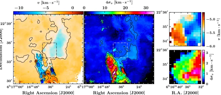
6h₁₇m₀₀s ₁₆m₄₈s ₃₆s ₂₄s 22◦₃₉0 360 330 300 Right ascension [J2000] Declination [J2000] 2.50 0.75− 1.1 pc IRAM 30m 12_CO(1_{− 0)} 22.500 3.

Fig. 6.Spitzer/MIPS map at 24.0 µm. In black contours, the emission of

12_{CO(2–1) observed with the IRAM 30 m is shown over different}

inter-vals of velocities: A [−7; −5] km s−1_{(cloudlet); B [−5.5; −4.5] km s}−1

(ring-like structure); and C and D [−40; +30] km s−1 _{(shocked clump}

and shocked knot). The white boxes represent the area where the sig-nal corresponding to each structure is integrated. The beam diameter of the IRAM 30 m observations of12_{CO(2–1) is shown in the bottom left}

corner.

structure might be incidental despite its remarkable features in the first moment map (Fig.5).

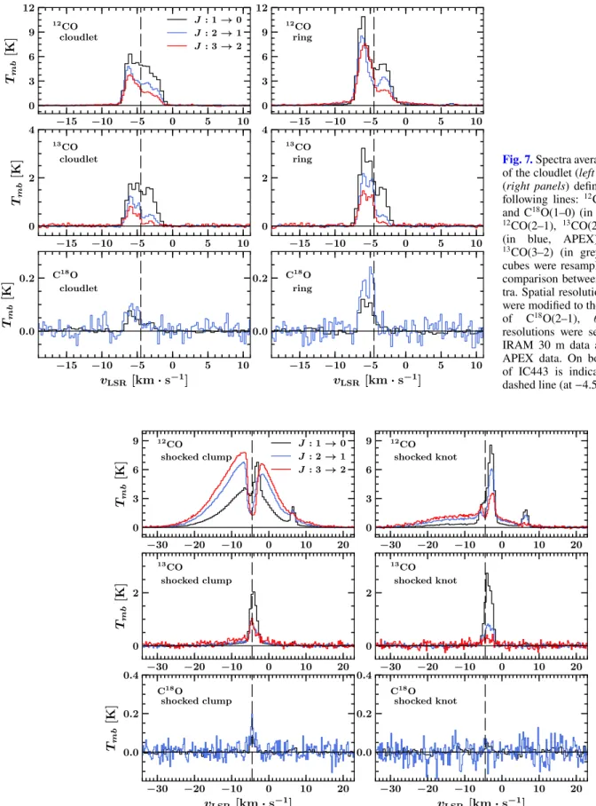
3. Shocked clump: considering the geometry of the SNR and the locally perpendicular direction of propagation of the SNR shockwave (van Dishoeck et al. 1993), the high-velocity emission arises from at least two shock waves, if not a col-lection of transverse shocks propagating along the molecular shell. In other words, the projection along the line of sight of several distinct shocked knots with distinct systematic veloci-ties could contribute to the broadening of the 12_{CO lines. We}

measure 3s ' 27 km s−1and 3s ' 21 km s−1 for the blueshifted

and redshifted transverse shocks, respectively. Except for the J = 1–0 spectrum for which the emission of the ambient gas con-tributes to the average spectra, all spectra of12_{CO lines exhibit}

a significant absorption feature around the 3LSR of IC443G,

suggesting that there is strong self-absorption of the emission lines. Evidence of line absorption is found in the velocity range −6 km s−1_{< v}_LSR_<_{−2 km s}−1_{, which is where we detect the}

spa-tially extended features associated with the NW-SE complex of molecular gas described byLee et al.(2012). Hence, it is pos-sible that the foreground cold molecular cloud is at the origin of the absorption of the12_{CO J = 1–0 and J = 2–1 lines. A faint}

and thin emission line is detected around 3 = 6.5 km s−1_{both in}

the 12_{CO and}13_{CO spectra. This signal is associated with the}

NE–SW complex of molecular gas described in Sect.3.2. 4. Shocked knot: the shock signature of this line is distinct from the shocked clump. As hinted by the moments map (Fig. 5), its fainter high-velocity wings are displaced toward negative velocities. A self-absorption feature is also observed in this structure. Between v = −5.5 km s−1 _{and v = −2 km s}−1

a bright and thin feature traces the ambient gas shown on the channel maps in Fig.2(second row from bottom; first, second and third panels from left).

The line width measured from the13_{CO line profiles when we}

consider only the spectral component that are physically asso-ciated with the cloudlet and ring-like structure (discarding the contribution of the ambient cloud) are 2.0 ± 0.3 km s−1 _and

1.6 ± 0.3 km s−1_{, respectively, measured by carefully defining}

much more constrained spatial boundaries around the struc-tures. From the average spectra presented in this section, there is no spectral evidence for the propagation of molecular shocks and/or outflows within these two structures, except for the faint wings displayed by the 12_{CO lines in the box associated with}

the ring-like structure. These extended wings arise from the contamination by the high-velocity emission of the shocked sub-structures that are contained in box B (Fig. 5). We measured the peak temperature, velocity centroid, FWHM, and area of the 12_{CO and}13_{CO lines J = 1–0, J = 2–1 and J = 3–2 in each}

average spectrum and report our results in Table3. 4.2. LTE method

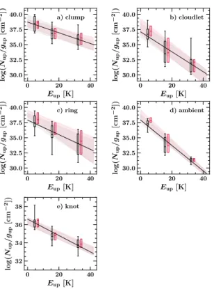
4.2.1. Two-dimensional histograms of CO data

In the next section, we aim to build population diagrams in which we correct the effect of optical depth on the column density of upper levels. To measure the optical depth of CO lines, we relied on several strong assumptions, in particular the adopted isotopic ratios and the identity of excitation temperature for12_CO

and13_{CO (see Sect.}_4.2.2_{for a description of our method, and}

Roueff et al. 2020for a complete discussion of the correspond-ing assumptions). To assess the validity of this approach and estimate the key parameters (isotopic ratios and excitation tem-perature ratios), we built 2D histograms from the12_{CO J = 1–0,}

J = 2–1, J = 3–2 data cubes, as well as13_{CO and C}18_{O J = 1–0}

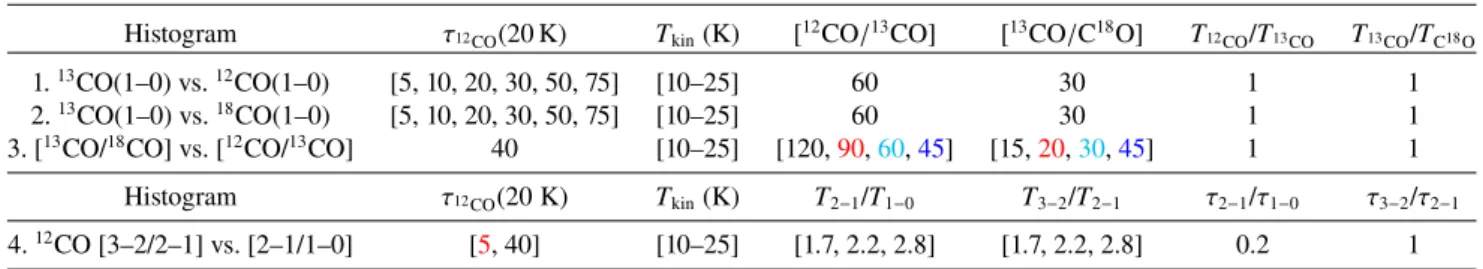
data cubes to compare the line intensity from different iso-topologs and rotational transitions of CO with modified LTE models (Bron et al. 2018). These assumptions are also discussed in Sect.4.2.3. We examined four different 2D data histograms:

1. J = 1–0 line intensity,13_{CO vs.}12_CO.

2. J = 1–0 line intensity,13_{CO vs. C}18_O.

3. J = 1–0 line intensity ratio, [13_CO/C18_{O] vs. [}12_CO/13_CO].

4. 12_{CO line intensity ratio, [3–2]/[2–1] vs. [2–1]/[1–0].}

In order to build the first three data histograms, we convolved all IRAM 30 m data cubes to the nominal spatial resolution of C18_{O(1–0) (i.e., 23.6}00_{) and to the nominal spectral resolution of}

the FTS backend (i.e., 0.5 km s−1_{). To build the fourth histogram,}

we resampled IRAM 30 m12_{CO(1–0), APEX}12_{CO(2–1), and}

APEX12_{CO(3–2) data cubes to the nominal spatial resolution}

of 12_{CO(1–0) (i.e., 22.5}00_{) and to the nominal spectral}

resolu-tion given by the FTS backend (i.e., 0.5 km s−1_{). We used a}

threshold of 3σ to select data points for which the signal is sig-nificantly above the noise level. The resulting 2D data histograms are shown in Fig.9.

Results. The first histogram is characterized by a high (S/N) ratio and represents a large statistical sample (n = 20 531). The13_{CO(1–0) vs.}12_{CO(1–0) relation presents at least two}

dis-tinct branches. The lower quasi-horizontal branch, tracing bright

12_{CO(1–0) emission associated with faint}13_{CO(1–0) line}

emis-sion (T13 <1 K km s−1). This branch is spatially correlated

with the shock structure and spectrally correlated with the high-velocity wings of the 12_{CO line, which have no bright} 13_CO

counterpart because of insufficient integration time. It is spa-tially correlated mainly with the quiescent molecular gas that is found within the cloudlet and ring-like structure and the ambient cloud.

(12)

−15 −10 −5 0 5 10 0 3 6 9 12 Tmb [K] 12_CO cloudlet J : 1→ 0 J : 2→ 1 J : 3→ 2 −15 −10 −5 0 5 10 0 2 4 Tmb [K] 13_CO cloudlet −15 −10 −5 0 5 10 vLSR [km· s−1] 0.0 0.2 Tmb [K] C18_O cloudlet −15 −10 −5 0 5 10 0 3 6 9 12 12_CO ring −15 −10 −5 0 5 10 0 2 4 13_CO ring −15 −10 −5 0 5 10 vLSR[km· s−1] 0.0 0.2 C18O ring

Fig. 7.Spectra averaged over the regions of the cloudlet (left panels) and the ring (right panels) defined in Fig.6for the following lines: 12_CO(1–0), 13_CO(1–0)

and C18_{O(1–0) (in black, IRAM-30m);} 12_CO(2–1), 13_{CO(2–1) and C}18_O(2–1)

(in blue, APEX); 12_{CO(3–2) and} 13_{CO(3–2) (in grey, APEX). Spectral}

cubes were resampled to allow a direct comparison between the different spec-tra. Spatial resolutions of all transitions were modified to the nominal resolution of C18_{O(2–1), θ = 30.2}00_{. Spectral}

resolutions were set to 0.5 km s−1 _for

IRAM 30 m data and 0.25 km s−1 _for

APEX data. On both panels, the 3LSR

of IC443 is indicated with a vertical dashed line (at −4.5 km s−1_).

−30 −20 −10 0 10 20 0 3 6 9 Tmb [K] 12_CO shocked clump J : 1→ 0 J : 2→ 1 J : 3→ 2 −30 −20 −10 0 10 20 0 2 Tmb [K] 13_CO shocked clump −30 −20 −10 0 10 20 vLSR[km· s−1] 0.0 0.2 0.4 Tmb [K] C18_O shocked clump −30 −20 −10 0 10 20 0 3 6 9 12_CO shocked knot −30 −20 −10 0 10 20 0 2 13_CO shocked knot −30 −20 −10 0 10 20 vLSR[km· s−1] 0.0 0.2 0.4 C18_O shocked knot

Fig. 8. Spectra averaged over the region of the shocked clump (left) and shocked knot (right) defined in Fig. 6 for the following lines:

12_CO(1–0),13_{CO(1–0) and C}18_{O(1–0) (in black, IRAM 30 m);}12_CO(2–1),13_{CO(2–1) and C}18_{O(2–1) (in blue, APEX);}12_{CO(3–2) and}13_CO(3–2)

(in grey, APEX). Spectral cubes were resampled to allow a direct comparison between the different spectra. Spatial resolutions of all transitions were modified to the nominal resolution of C18_{O(2–1), θ = 30.2}00_{. Spectral resolutions were set to 0.5 km s}−1_{for IRAM 30 m data and 0.25 km s}−1

(13)

Table 3. Summary of the spectral characteristics of the lines of12_{CO and}13_{CO within the boxes corresponding to each structures, defined in Fig.}₆_.

12_CO 13_CO

Region Ju− Jl T_mb∗ 30 3FWHM Area T_mb∗ 30 3FWHM Area

(K) (km s−1₎ _{(km s}−1_{) (K km s}−1₎ _(K) _{(km s}−1₎ _{(km s}−1_{) (K km s}−1₎ Cloudlet 1–0 6.1 ± 0.1 −5.8 ± 0.2 2.1 ± 0.3 15.5 ± 0.3 1.7 ± 0.1 −5.6 ± 0.2 2.0 ± 0.2 4.1 ± 0.1 α =6h16m30s 2–1 4.7 ± 0.1 −5.9 ± 0.3 1.9 ± 0.3 9.7 ± 0.2 1.1 ± 0.1 −5.7 ± 0.3 1.8 ± 0.2 1.7 ± 0.3 δ =22◦₃₆0₀₀00 _3–2 _{3.5 ± 0.1} _{−6.1 ± 0.2 1.6 ± 0.2 6.9 ± 0.2} _{0.8 ± 0.1 −5.8 ± 0.3 2.2 ± 0.3 1.2 ± 0.1} Ring 1–0 11.7 ± 0.2 −6.0 ± 0.2 1.6 ± 0.2 20.1 ± 0.3 3.5 ± 0.1 −5.7 ± 0.2 1.7 ± 0.2 5.8 ± 0.2 α =6h₁₆m₃₆s _2–1 _{9.5 ± 0.1} _{−6.1 ± 0.1 1.4 ± 0.2 14.3 ± 0.2} _{2.8 ± 0.1 −5.5 ± 0.2 1.6 ± 0.2 3.6 ± 0.1} δ =22◦3404000 3–2 9.5 ± 0.1 −5.7 ± 0.3 1.9 ± 0.2 15.0 ± 0.3 1.8 ± 0.1 −5.5 ± 0.3 1.7 ± 0.3 2.5 ± 0.1 Shocked clump 1–0 7.1 ± 0.1 −6 ± 1 19 ± 1 49.7 ± 0.4 2.5 ± 0.1 −3.8 ± 0.1 2.1 ± 0.1 6.5 ± 0.1 α =6h₁₆m₄₂s _2–1 _{5.2 ± 0.1} _{−7 ± 1} _{23 ± 1} _{71 ± 1} _{0.8 ± 0.1 −3.8 ± 0.2 2.4 ± 0.2 3.5 ± 0.1} δ =22◦3200000 3–2 4.9 ± 0.1 −7 ± 1 24 ± 1 80 ± 1 0.7 ± 0.1 −4.4 ± 0.2 1.4 ± 0.2 4.5 ± 0.2 Shocked knot 1–0 8.8 ± 0.1 −8 ± 2 17 ± 1 18.8 ± 0.2 2.4 ± 0.1 −3.7 ± 0.1 2.4 ± 0.1 7.5 ± 0.1 α =6h₁₆m₄₂s _2–1 _{6.0 ± 0.1} _{−9 ± 2} _{21 ± 1} _{21.1 ± 0.3} _{0.7 ± 0.1 −3.5 ± 0.2 2.6 ± 0.3 3.2 ± 0.1} δ =22◦3200000 3–2 3.4 ± 0.1 −9 ± 2 22 ± 1 24.4 ± 0.4 0.3 ± 0.1 −3.9 ± 0.3 1.9 ± 0.3 1.3 ± 0.5 Notes. T∗

mbis the peak temperature of the line, 30is the centroid, and vFWHMthe line width. The quantity Tmb∗ and the area are directly measured

from reading the spectral data. The quantities vFWHMand 30are measured by modeling the line either by a single or double Gaussian function that

best fits the data. When two Gaussian functions are needed to model the sum of the signal emitted by the ambient cloud and structure of interest, we discard the contribution of the ambient cloud and only take into account the parameters 30and 3FWHMassociated with the broad component. The

asymmetric high-velocity wings of12_{CO lines corresponding to the shocked clump require two Gaussians, thus we measure 3}

0=(c1+c2)/2 and

3FWHM=p((2.355 σ1)2+(2.355 σ2)2), where c1, c2, σ1, and σ2are the centroids and standard deviations corresponding to each Gaussian function,

respectively. 0 10 20 12_CO(1_{− 0) [K · km/s]} 0 2 4 6 8 13 CO(1 − 0) [K · km / s] 1. τ = 5 τ = 10 τ = 20 τ = 30 τ = 50 τ = 75 Tkin= 10− 25 K [12_CO]/[13_{CO] = 60} [13_CO]/[C18_{O] = 30} 0.0 0.2 0.4 0.6 C18_O(1_{− 0) [K · km/s]} 0 2 4 6 8 10 13 CO(1 − 0) [K · km / s] 2. 510 20 30 50 75 Tkin= 10− 25 K [12_CO]/[13_{CO] = 60} [13_CO]/[C18_{O] = 30} 100 ₁₀1 12_CO/13_CO 100 101 13 CO / C 18 O 3. Tkin= 10− 25 K τ = 40 [12_CO]/[13_CO] = 120, 90, 60, 45 [13_CO]/[C18_O] = 15, 20, 30, 45 − −− − −− 0 2 4 6 12_{CO[J = 2}_{− 1/J = 1 − 0]} 0 2 4 6 12 CO[ J = 3 − 2 /J = 2 − 1] 4. 1.7 2.2 2.8 Tkin= 10− 25 K τ = 5 τ = 40− T2−1/T1−0 = 1.7, 2.2, 2.8 T3−2/T2−1 = 1.7, 2.2, 2.8 100 101 102 100 101 100 101 100 101 102 103

Fig. 9. Data histograms and LTE models of the emission of the rotational transitions of12_{CO and its isotopologs mapped in the extended G}

field with the IRAM 30 m and APEX: 1.13_{CO(1–0) vs.}12_{CO(1–0); 2.}13_{CO(1–0) vs. C}18_{O(1–0); 3. [}13_{CO(1–0)] / [C}18_{O(1–0)] vs. [}12_CO(1–0)]

/ [13_{CO(1–0)]; and 4.}12_{CO(3–2) /}12_{CO(2–1) vs.}12_{CO(2–1) /}12_{CO(1–0). The color map corresponds to the amount of data points (line of sight}

and velocity channels) that fall into a given bin of the histogram. The curves represent families of models of the LTE intensity as a function of the kinetic temperature of13_{CO. The arrows indicate the direction in which the kinetic temperature grows along a given curve. Control parameters of}

the LTE models are given in Table4for each histogram. The dashed black lines represent the 3σ detection level for each axis (histograms 1 and 2).

The13_{CO(1–0) vs. C}18_{O(1–0) histogram has a much smaller}

number of bins determined with a good (S/N) (n = 833) due to the faint emission of C18_{O(1–0) that is hardly detected at a 3σ}

confidence level within our data cube. Still, we find evidence of at least one statistically significant branch. As a result of to the small size of the sample, it is not possible to identify any spatial or spectral correlation with certainty.

The third histogram has a poor statistical sample for the same reason as the second one (n = 833). The [13_CO(1–0)]/

[C18_{O(1–0)] ratio vs. [}12_CO(1–0)]/[13_{CO(1–0)] relationship is}

localized in an area with little dispersion. Hence, for high signal-to-noise measurements the isotopic ratios are almost uniform in the field of observations. Nonetheless, the lower signal-to-noise data bins display a statistically well-defined comet-shaped