HAL Id: hal-02394984
https://hal.archives-ouvertes.fr/hal-02394984
Submitted on 11 Dec 2019
HAL is a multi-disciplinary open access archive for the deposit and dissemination of sci-entific research documents, whether they are pub-lished or not. The documents may come from teaching and research institutions in France or abroad, or from public or private research centers.
L’archive ouverte pluridisciplinaire HAL, est destinée au dépôt et à la diffusion de documents scientifiques de niveau recherche, publiés ou non, émanant des établissements d’enseignement et de recherche français ou étrangers, des laboratoires publics ou privés.
OBSERVATIONS AND NUMERICAL MODEL
RESULTS OF MORPHODYNAMIC FEEDBACK
OWING TO WAVE-CURRENT INTERACTION
J Hopkins, M de Schipper, M Wengrove, F de Wit, B. Castelle
To cite this version:
J Hopkins, M de Schipper, M Wengrove, F de Wit, B. Castelle. OBSERVATIONS AND NUMERICAL MODEL RESULTS OF MORPHODYNAMIC FEEDBACK OWING TO WAVE-CURRENT INTER-ACTION. Coastal Sediments’19, May 2019, Tampa, United States. �10.1142/9789811204487_0049�. �hal-02394984�
1
OBSERVATIONS AND NUMERICAL MODEL RESULTS OF MORPHODYNAMIC FEEDBACK OWING TO WAVE-CURRENT
INTERACTION
J. Hopkins1, M.A. de Schipper1, M. Wengrove2, F. de Wit1, B. Castelle3 1Delft University, [email protected], [email protected], F.p,[email protected] 2Oregon State University, [email protected]
3University of Bordeaux [email protected]
Abstract: Predicting the evolution of mound formations in the nearshore, both natural (e.g. bars) and man-made (e.g. nourishments) requires an understanding of mixed wave-current flow on sediment transport. MODEX (Morphological Diffusivity EXperiment) used a wave-current-sediment flume to capture detailed spatial and temporal observations of sand mound evolution in shallow water. Imposed flow included waves-alone, currents-alone, and combined wave-currents. MODEX provides a test bed for understanding the impact of currents on waves around submerged bedforms and the feedback with morphology. Here, a wave-resolving model SWASH is used to simulate flow patterns around the mound as it diffuses, showing the impact of wave-current interaction on both mound evolution and scouring observed around the mound. Further, simulations initialized with a diffused mound show the feedback between 3D bed deformation and wave-current flow structures. The results provide a framework for understanding and implementing intra-wave sediment transport in wave-resolving models. Extensions of the results to field conditions with mixed wave-current energy will be explored.
Introduction
The accurate characterization of nearshore sediment transport around a mound is critical to predict the fate of foreshore nourishments, which can inform better management practices for sandy coastlines. To date, the evolution of submerged nearshore mounds (or bars) has been investigated on a variety of scales, with field studies observing the behaviour of bathymetric perturbations in a range of conditions (Gallagher et al., 1998; Ruessink et al., 2000; Ruggiero et al., 2009, among others) and laboratory studies investigating the detailed physical processes underlying the movement of sand in wave and current conditions (Drake et al., 1992; Grant & Madsen, 1982; Yuan & Madsen, 2014, among others). Both approaches have advanced our ability to design nourishments (field) and calculate sediment transport under waves and currents (laboratory) yet each has limitations. Large-scale field studies require intensive observations to capture and untangle the complex interplay of forcing and response of a submerged mound. Small-scale
2
laboratory studies investigating boundary layer effects give insight into the shear stress generated by specific wave and current conditions but are difficult to scale up to the field.
Field studies focused on observing full-scale nourishments tend to capture the general behavior (accrete, erode, move shoreward or not) shown to have reasonable agreement with water depth and wave height [Hands et al., 1997; Boers, 2005] and can broadly inform the choice of future nourishment locations. An experiment at Duck, NC which monitored the inverse problem of a mound, the evolution of holes dug into the surf zone, linked morphological evolution to gravity-driven slope effects [Moulton et al., 2014] and calculated a diffusion parameter for downslope transport to be used in wave-averaged models such as Delft3D and XBeach [Lesser
et al., 2004; Harter and Figlus, 2017]. Further, the parametrization of down-slope
sediment transport was found critical to model the morphodynamics of sandbars in the surfzone [Dubarbier et al., 2017].
In an attempt to link this general behavior to sediment dynamics, laboratory studies investigating the evolution of artificial mounds in wave flumes have been conducted in a narrow range of hydrodynamic wave conditions, the results of which show reasonable agreement with wave-averaging numerical models [Stansby et al., 2009;
Smith et al., 2017; Ruol et al., 2018]. To expand the hydrodynamic range and better
characterize the diffusive behavior of a submerged nearshore mound, MODEX (Morphological Diffusivity EXperiment) was conducted in Summer 2018 to monitor in detail the evolution of a single mound under a variety of wave, current, and combined forcing conditions.
The seven-week flume experiment was designed to capture the diffusion of a Gaussian mound with fine spatial and temporal resolution, monitoring how waves and currents transform over the mound as well as the 3D evolution of the mound over time. In this paper, we explain the method for collecting temporally dense bathymetry data of the mound evolution, and use this data to force a wave-resolving model SWASH (Simulating WAves till SHore) to capture the hydrodynamic transformation as the mound evolves. The choice of this model allows for simulations of the detailed feedback between mound shape and hydrodynamic conditions such as wave refraction and vertical velocity structure under individual waves, which in turn inform predictions of how this mound and similar ones in the field will evolve over time.
3
This paper introduces preliminary validation and results from model-data simulations. Accompanying papers in this proceedings (see de Schipper et al., 2019
and Lee et al., 2019) give more detail into the complete MODEX experiment and
associated hydrodynamic observations.
Methods
Experiment Setup
MODEX took place in a 6x12m flume in the Total Environment Simulator in Hull, UK. The experiment (Figure 1) began with a 1.5m diameter, 20cm high sandy mound placed in the middle of a bed of sand 10cm deep. The flume was filled with 40cm of water and a sequence of waves and currents, either alone or combined, were run over the mound until the mound height was approximately half its original.
Figure 1: (a) side view and (b) top view of experimental design, where (a) 10cm of sand covers the bed
of the flume with 40cm of water above and (b) a 1.5m diameter mound 20cm high is placed in the center of the flume equidistant from the wave maker (to the right in (a) and (b)).
4
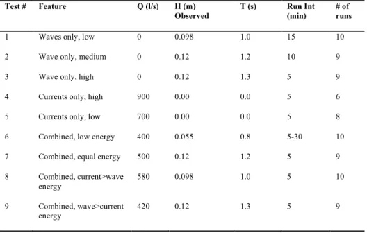
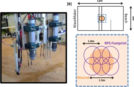
Nine hydrodynamic conditions were tested over identical sandy mounds, including three with waves alone, two with currents alone, and four with mixed wave and current conditions (Table 1). The morphodynamic evolution of the mound was tracked using an innovative system of Marine Electronics ripple profiling scanners (RPS), capable of capturing the 3D bathymetric evolution of the mound (Figure 2). Two RPS were mounted above the mound on a moving gantry. During flow, the RPS were raised above the water level to minimize disturbance to the waves and currents. The flow was stopped every 5-15 minutes for the two RPS to be lowered into the water. Each instrument had a meter diameter footprint owing to the shallow water depth (Figure 2), so the gantry was moved along the length of the flume to allow for the full mound footprint to be captured. Once a set of RPS scans completed, the RPS were raised out of the water and the flow was run again for another 5-15 minutes.
Table 1: List of test runs and associated hydrodynamic conditions, including flow rate (Q), wave height
(H), wave period (T), and run time for the flow between RPS scanning intervals.
Test # Feature Q (l/s) H (m) Observed T (s) Run Int (min) # of runs
1 Waves only, low 0 0.098 1.0 15 10
2 Wave only, medium 0 0.12 1.2 10 9
3 Wave only, high 0 0.12 1.3 5 9
4 Currents only, high 900 0.00 0.0 5 6
5 Currents only, low 700 0.00 0.0 5 8
6 Combined, low energy 400 0.055 0.8 5-30 10
7 Combined, equal energy 500 0.12 1.2 5 9
8 Combined, current>wave energy
580 0.098 1.0 5 10
9 Combined, wave>current
5
Figure 2: (a) Image of the two ripple profiling scanners used to track bed level through a series of scans
with (b) 1m footprints. This resulted in six scans (three per instrument) over the mound achieved by moving a gantry (two parallel lines in (b) top image) along the flume in 50cm increments. The timing of the scans depended on the strength of the flow conditions. Low energy flow required 15 minutes of waves and currents between scans to see changes in mound morphology. High energy flow evolved rapidly, so scans were done every 5 minutes. This resulted in roughly nine sets of RPS scans for each test, with each set consisting of six individual RPS footprints.
The bed level from the footprints was determined from the highest return value in the RPS backscatter data [Wengrove et al., 2018]. Post-processing consisted of stitching the six individual footprints into one complete image of the mound. Each RPS was rotated slightly off the long axis of the flume. This was corrected and the footprints overlaid to form a snapshot of the mound (Figure 3). Since the water level was shallow, the highest return value did not always correspond to the bed, so the final scans had to be cleaned for outliers. The result from one test was a complete set of scans showing mound diffusion at regular intervals (Figure 4).
6
Figure 3: Image of the mound from the start of Test 1 stitched together using six RPS scans.
Color scale is depth in meters for visual aid of mound height.
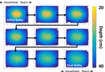
Figure 4: Sequence of RPS scans taken over the course of Test 2 (Table 1) from the initial bathymetry
(top left) following the black arrows every 10 minutes to the final bathymetry (bottom right). Colored contours represent depth in centimeters.
7
SWASH Model Setup
The bathymetry scans were used to initialize the wave-resolving SWASH model to test the feedback between morphology and flow structure around the mound. SWASH is a hydrodynamic model which solves the nonlinear shallow water equations with non-hydrostatic pressure, and includes a 𝜅 − 𝜖 turbulence model [Zijlema et al., 2011]. The model can simulate individual wave crests as well as currents in the water column. As such, it is a reasonable choice for the dynamics of the combination of forcings used in MODEX.
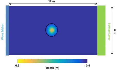
The MODEX SWASH model is initialized with the mound bathymetry in the flume (Figure 5) scanned by the RPS. At one end of the model domain is a wave maker (and current generator), at the other end is a sponge layer (for waves) or outflow (currents). The along-flow sides of the flume are periodic to prevent non-physical wave reflection in the domain. The model is run with default settings outside of the bathymetry and boundary conditions. The grid resolution is 3cm in the horizontal and results are shown here for a model with one vertical layer.
Figure 5: Model domain, including the bathymetry used to initialize the SWASH model. The mound is
outlined in black and located in the center of the model (as it was in the center of the flume). The mound shape (colored contours) is adapted from RPS scans. This image shows the mound at the beginning of a
8
Model bathymetry are constructed from RPS scans taken over the course of a test (Figure 4) to track how the flow conditions change in response to the mound shape. Three types of conditions are simulated: wave-only, current-only, and wave-current combined. For waves alone, the boundary conditions are a wave maker which imposes linear sinusoidal waves uniformly on one side of the domain (light blue bar in Figure 5) with a prescribed wave period and height (directed in the long axis of the flume) and a sponge layer extending the domain back 6m (green bar, not to scale, in Figure 5). For currents alone, the boundary conditions are discharge on the wave maker side of the flume (light blue bar in Figure 5) and a radiation boundary condition on the outflow side (light green bar in Figure 5). The water depth is set by the imposed bathymetry.
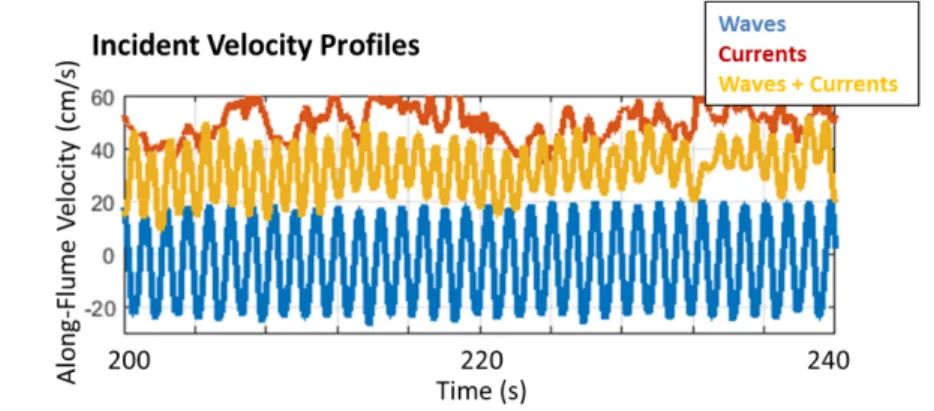
Wave-current combined tests require some finesse with the boundary conditions. At present, SWASH does not allow two boundary conditions to be simultaneously imposed on one side of the domain. To feed the model both waves and currents, we constructed time series of velocity based on observed wave-current conditions in the flume before the mound (Figure 6, orange line). These observed conditions capture wave-current interaction effects such as elongating and shortening of waves owing to a following current. The opposite boundary condition was set to a discharge equal to a moving average of velocity taken (window length 10s) from the input conditions.
Figure 6: Along-flume velocity measured before the flow encountered the mound for (blue line) waves
alone, Test 2, (red line) currents alone, Test 5, and (orange line) wave-currents combined, Test 8. Note that the discharge in Test 5 (red line) is higher than Test 8 (orange line).
9
Preliminary Results
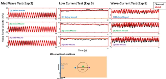
Figure 7: Observed (black) vs. modelled (red) along-flume flow velocity for instruments located (a,d,g)
before the mound (blue dot in the inset mound map), (b,e,h) above the mound (green dot), and (c,f,i) behind the mound. Simulations of (a,b,c) waves alone and (d,e,f) currents alone agree well with observed results. Simulations of (g,h,i) wave-current interaction have reasonable agreement, though the model does not fully capture the wave transformation (i) behind the mound in terms of adjustments to wave period
and skewness.
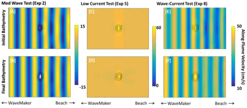
SWASH reproduces wave and current conditions in the flume (Figure 7, compare black and red lines) with velocities in the range observed during experimental runs (Figure 6, Figure 7 black lines). Further, the spatial density of model output (Figure 8) shows flow reacting to the presence of the mound both through wave refraction (Figure 8a,c) and flow contraction (Figure 8b,d). These effects diminish as the mound diffuses (compare Figure 8a,c to 8b,d). For the wave-current tests (Figure 8e,f) flow conditions again appear more uniform as the mound diffuses, with stronger refraction and skewness behind the mound seen in the initial bathymetry (Figure 8e) as compared to the final bathymetry (Figure 8f).
10
Figure 8: Along-flume velocity (colored contours) output from SWASH for (a,b) wave conditions from
Test 2 (see Table 1), (c,d) current conditions from Test 5 (see Table 1) and (e,f) wave-current conditions from Test 8 (see Table 1) both (a,c,e) during the first test run and (b,d,f) during the final run of the experiment. The model shows how flow conditions around the mound change as the mound diffuses. In the wave-alone case (a,b) show less refraction owing to mound diffusion, while in the current-alone case (b,d,) the velocity field becomes more uniform as the mound diffuses. For the wave-current case (e,f,) wave refraction and skewness are evident as wave troughs deepen behind the mound. Black contour lines
indicate mound bathymetry (contour ever 10cm) and location.
These model simulations will be used to determine the feedback between mound bathymetry and wave-current effects, tracking how the hydrodynamics respond to mound diffusion and, as a result, how drivers of sediment transport change over a test run. Model runs will cover a range of wave-current conditions to determine how the balance of these forcings influences mound diffusion.
Concluding Remarks
Detailed 3D scans of a sandy mound subject to wave and current forcing show mound diffusion at fine temporal resolution. These scans are used in a wave-resolving model to explore the feedback between waves, currents, combined conditions, and the mound shape as it evolves. Initial model results show how flow structure becomes more uniform as the mound evolves, with more complex initial structure (wave refraction and skewness) apparent in combined wave-current cases. Model results will be extended to three-dimensions and used to show how varying ratios of wave-current energy force mound evolution, determining thresholds at which each begin to dominate the eventual mound smoothing and planform shape.
11
Acknowledgements
This research was made possible by the excellent team at the Total Environment Simulator (TES) in Hull, UK. Stuart McClelland, Brendan Murphy, Hannah Williams, and Laura Jordan were instrumental in experimental set up and smooth execution. Scientific contributions from visitors Anne Baar and Seok-Bong Lee were crucial to understand flow data and capture more precise measurements.
References
Boers, M. (2005), Overview of historical pits, trenches and dumpsites on the NCS, in SANDPIT: Sand transport and morphology of offshore sand mining pits, edited by L. C. van Rijn, R. L. Soulsby, P. Hoekstra, and A. G. Davies, Aqua Publications, the Netherlands.
Drake, D. E., D. A. Cacchione, and W. D. Grant (1992), Shear stress and bed roughness estimates for combined wave and current flows over a rippled bed,
J. Geophys. Res., 97(C2), 2319.
Dubarbier, B., B. Castelle, G. Ruessink, and V. Marieu (2017), Mechanisms controlling the complete accretionary beach state sequence, Geophys. Res.
Lett., 44(11), 5645–5654.
Gallagher, E. L., S. Elgar, and R. T. Guza (1998), Observations of sand bar evolution on a natural beach, J. Geophys. Res., 103(C2), 3202–3215.
Grant, W. D., and O. S. Madsen (1982), Movable bed roughness in unsteady oscillatory flow, J. Geophys. Res., 87(C1), 469.
Hands, E. B., J. P. Ahrens, and D. T. Resio (1997), Predicting Large-Scale, Cross-Shore Sediment Movement from Orbital Speeds, in Coastal Engineering
1996, pp. 3378–3390, American Society of Civil Engineers, New York, NY.
Harter, C., and J. Figlus (2017), Numerical modeling of the morphodynamic response of a low-lying barrier island beach and foredune system inundated during Hurricane Ike using XBeach and CSHORE, Coast. Eng., 120(April 2016), 64–74.
12
Lesser, G. R., J. A. Roelvink, J. a. T. M. van Kester, and G. S. Stelling (2004), Development and validation of a three-dimensional morphological model,
Coast. Eng., 51, 883–915.
Moulton, M., S. Elgar, and B. Raubenheimer (2014), A surfzone morphological diffusivity estimated from the evolution of excavated holes, Geophys. Res.
Lett., 41(13), 4628–4636.
Ruessink, B., I. M. van Enckevort, K. Kingston, and M. Davidson (2000), Analysis of observed two- and three-dimensional nearshore bar behaviour, Mar. Geol.,
169(1–2), 161–183.
Ruggiero, P., D. J. R. Walstra, G. Gelfenbaum, and M. van Ormondt (2009), Seasonal-scale nearshore morphological evolution: Field observations and numerical modeling, Coast. Eng., 56(11–12), 1153–1172.
Ruol, P., L. Martinelli, C. Favaretto, and D. Scroccaro (2018), Innovative Sand Groin Beach Nourishment With Environmental, Defense and Recreational Purposes, in The 28th International Ocean and Polar Engineering
Conference, International Society of Offshore and Polar Engineers, Sapporo.
Smith, E. R., M. C. Mohr, and S. A. Chader (2017), Laboratory experiments on beach change due to nearshore mound placement, Coast. Eng., 121, 119–128. Stansby, P. K., J. Huang, D. D. Apsley, M. I. García-Hermosa, A. G. L. Borthwick,
P. H. Taylor, and R. L. Soulsby (2009), Fundamental study for morphodynamic modelling: Sand mounds in oscillatory flows, Coast. Eng.,
56(4), 408–418.
Wengrove, M. E., D. L. Foster, T. C. Lippmann, M. A. de Schipper, and J. Calantoni (2018), Observations of Time-Dependent Bedform Transformation in Combined Wave-Current Flows, J. Geophys. Res. Ocean., 123(10), 7581– 7598.
Yuan, J., and O. S. Madsen (2014), Experimental study of turbulent oscillatory boundary layers in an oscillating water tunnel, Coast. Eng., 89, 63–84.
13
domain code for simulating wave fields and rapidly varied flows in coastal waters, Coast. Eng., 58(10), 992–1012.