Nonstationarity of strong collisionless quasiperpendicular shocks: Theory and full particle numerical simulations

HAL Id: insu-02928445

https://hal-insu.archives-ouvertes.fr/insu-02928445

Submitted on 2 Sep 2020

HAL is a multi-disciplinary open access

archive for the deposit and dissemination of

sci-entific research documents, whether they are

pub-lished or not. The documents may come from

teaching and research institutions in France or

abroad, or from public or private research centers.

L’archive ouverte pluridisciplinaire HAL, est

destinée au dépôt et à la diffusion de documents

scientifiques de niveau recherche, publiés ou non,

émanant des établissements d’enseignement et de

recherche français ou étrangers, des laboratoires

publics ou privés.

Nonstationarity of strong collisionless

quasiperpendicular shocks: Theory and full particle

numerical simulations

Vladimir Krasnoselskikh, Bertrand Lembège, P. Savoini, V. V. Lobzin

To cite this version:

Vladimir Krasnoselskikh, Bertrand Lembège, P. Savoini, V. V. Lobzin. Nonstationarity of strong

col-lisionless quasiperpendicular shocks: Theory and full particle numerical simulations. Physics of

Plas-mas, American Institute of Physics, 2002, 9 (4), pp.1192-1209. �10.1063/1.1457465�. �insu-02928445�

Physics of Plasmas 9, 1192 (2002); https://doi.org/10.1063/1.1457465 9, 1192

© 2002 American Institute of Physics.

Nonstationarity of strong collisionless

quasiperpendicular shocks: Theory and full

particle numerical simulations

Cite as: Physics of Plasmas 9, 1192 (2002); https://doi.org/10.1063/1.1457465

Submitted: 05 June 2001 . Accepted: 09 January 2002 . Published Online: 21 March 2002 V. V. Krasnoselskikh, B. Lembège, P. Savoini, and V. V. Lobzin

ARTICLES YOU MAY BE INTERESTED IN

Shock front instability associated with reflected ions at the perpendicular shock

Physics of Plasmas 14, 012108 (2007); https://doi.org/10.1063/1.2435317

Whistler waves, core ion heating, and nonstationarity in oblique collisionless shocks

Physics of Plasmas 14, 072103 (2007); https://doi.org/10.1063/1.2748391

Nonstationarity of a two-dimensional quasiperpendicular supercritical collisionless shock by self-reformation

Nonstationarity of strong collisionless quasiperpendicular shocks:

Theory and full particle numerical simulations

V. V. Krasnoselskikha)

LPCE/CNRS, Orle´ans, France

B. Lembe`ge and P. Savoini

CETP/CNRS, Velizy, France

V. V. Lobzinb)

LPCE/CNRS, Orle´ans, France

共Received 5 June 2001; accepted 9 January 2002兲

Whistler waves are an intrinsic feature of the oblique quasiperpendicular collisionless shock waves. For supercritical shock waves, the ramp region, where an abrupt increase of the magnetic field occurs, can be treated as a nonlinear whistler wave of large amplitude. In addition, oblique shock waves can possess a linear whistler precursor. There exist two critical Mach numbers related to the whistler components of the shock wave, the first is known as a whistler critical Mach number and the second can be referred to as a nonlinear whistler critical Mach number. When the whistler critical Much number is exceeded, a stationary linear wave train cannot stand ahead of the ramp. Above the nonlinear whistler critical Mach number, the stationary nonlinear wave train cannot exist anymore within the shock front. This happens when the nonlinear wave steepening cannot be balanced by the effects of the dispersion and dissipation. In this case nonlinear wave train becomes unstable with respect to overturning. In the present paper it is shown that the nonlinear whistler critical Mach number corresponds to the transition between stationary and nonstationary dynamical behavior of the shock wave. The results of the computer simulations making use of the 1D full particle electromagnetic code demonstrate that the transition to the nonstationarity of the shock front structure is always accompanied by the disappearance of the whistler wave train within the shock front. Using the two-fluid MHD equations, the structure of nonlinear whistler waves in plasmas with finite beta is investigated and the nonlinear whistler critical Mach number is determined. It is suggested a new more general proof of the criteria for small amplitude linear precursor or wake wave trains to exist. © 2002 American Institute of Physics. 关DOI: 10.1063/1.1457465兴

I. INTRODUCTION

Shock waves in plasmas as well as in gases and other media are usually considered to be nonlinear waves that cause changes of state of the media and are stationary in some reference frames. Indeed, numerous theoretical papers are devoted to finding stationary solutions to the set of equa-tions describing the plasma dynamics共for a review, see, e.g., Refs. 1–3兲. However, in the very beginning of the collision-less shock physics, the hypothesis was suggested that high Mach number shocks can be nonstationary共see, e.g., Refs. 4, 5兲. As far as we know, the first unambiguous evidence of the shock wave nonstationarity was obtained by Morse et al.6in the laboratory experiments with a plasma-wind-tunnel de-vice. They revealed that in the fast mode Mach number range

Mf⯝4 –8 the shock wave oscillates with a frequency

com-parable to the upstream ion gyrofrequency.

In the early 1980s, in the response both to new observa-tions of the Earth bow shock and a great progress both in computational sciences and computer hardware, the interest to the problem concerned is considerably increased. In the

Earth bow shock, the low frequency oscillations of the ion flux were observed.7–9 Later similar phenomenon was also found in the uranium bow shock.10 These observations can easily be interpreted as a manifestation of the shock front nonstationarity.11,12In addition, Leroy et al.13,14modeled the dynamics of a perpendicular shocks with the use of a hybrid code. Simulations with the parameters typical for the Earth bow shock共in particular, for M_A⫽8 and␤_e⫽␤_i⫽0.6, where

M_A is the Alfve´n Mach number,␤_e,iis the ratio of the ther-mal and magnetic pressures兲 showed that the shock structure varies with time, for example, the maximum value of the magnetic field exhibits temporal variations with a character-istic time of the order of ion gyroperiod, the magnitude of these variations being about of 20%. The amplitude of the oscillations increases with the Mach number and decreasing

␤i. The oscillations of the fraction of reflected ions,␣, are

more pronounced than that of the magnetic field overshoot or the maximum value of electric potential. For M_A⫽10 and

␤⫽0.1 the ion reflection was bursty, ␣ oscillating between 0% and 70%–75%, although the magnetic field and electric potential overshoot can be considered as quasistationary on the average because their relative amplitudes of oscillations do not exceed 10%–15%.

For the first time, modeling of high Mach number

per-a兲_{Electronic mail: vkrasnos@cnrs-orleans.fr}

b兲_{Permanent address: IZMIRAN, Troitsk, Moscow Region, Russia.}

1192

pendicular shocks ( M_A⫽22, ␤⫽0.1) was carried out by Quest.15 He found that in the absence of the electron resis-tivity the ion reflection process is periodic, the stages with 100% ion reflection alternating with the stages of 100% ion transmission. As a result, a periodic shock front reformation was observed rather than a stationary structure. Quest16 ex-tended these preliminary simulations to perform a systematic study of high Mach number perpendicular shocks. For ␤

⫽0.1 he revealed that the found previously14 _{tendency for a}

shock to become increasingly time-dependent as M_A in-creases was also observed for M_A⭓10 and resulted in the cyclical wave breaking for M_A⭓20. In addition, for ␤⫽1 and M_A⭓10 a non-trivial dependence of the shock front structure on the resistivity was found. Nonstationarity was observed both for low and high resistivity ␩ while for mod-erate␩the shocks were stationary up to MA⫽60. In

conclu-sion, Quest16 argued that a fundamental question concerned with a physical mechanism that controls the stability of the shocks has not been resolved yet.

In addition, it is worth noting that in numerical simula-tions the intrinsic shock front instability can be obscured by a number of unphysical effects such as an artificial dissipa-tion, dispersion, and/or instability of the computational algorithm.11

Analyzing the major achievements of collisionless shock physics by the end of 1984 and reviewing the conceptual issues of the subject, Kennel et al.17 argued that the shock front nonstationarity does exist and they suggested to intro-duce the so-called third critical Mach number corresponding to the transition between the stationary shocks and nonsta-tionary ones.

Krasnoselskikh18and Galeev et al.19suggested the theo-retical models describing the shock front instability due to domination of the nonlinear effects over the dispersion and dissipation. This instability results in a gradient catastrophe within a finite time interval and nonstationarity of the shock wave. Later Galeev et al.20 showed that the nonlinear whis-tler wave train can be observed within the front of the qua-siperpendicular shock wave under some conditions and they argued that the role of this wave train should be taken into account when analyzing the problem concerned. To confirm the hypothesis of shock front nonstationarity, Galeev et al.11 presented the results of analysis of the experimental data obtained onboard Prognoz-8 and Prognoz-10 for several crossings of the Earth bow shock. The manifestation of the shock front nonstationarity in the ion distribution function was also discussed.12Later, the presence of the nonstationary whistler wave trains in the front of strong quasiperpendicular shock waves was also confirmed by direct observations of the Earth bow shock onboard Intershock-Prognoz-10 and AMPTE UK spacecrafts.21

Lembe´ge et al.22also observed the cyclic reformation of the exactly perpendicular low-beta nonresistive shock waves in 1D full particle simulations, where the ratio of electron and ion masses was ␮⫽me/mi⫽0.01. They argue that very

high Mach numbers are not necessary for the reformation to exist; in these simulations the reformation was also observed for relatively low Mach numbers MA⫽2 –3 corresponding

however to supercritical regimes. In the 2D full particle

simulations with the mass ratio ␮⫽0.024, Lembe´ge et al.23 found that the cyclic reformation of the front takes place also for oblique shock waves within the same Mach number range even when the finite resistivity effects due to cross-field-current instabilities are self-consistently included. The reformation cycle was found to be of the order of the mean ion gyroperiod measured in the shock ramp. Furthermore, the shock front appeared to be rippled rather than uniform. However, the discussion of these two-dimensional effects is beyond the scope of the present paper.

The present paper is organized as follows: In Sec. II, the model suggested in Ref. 19 is briefly outlined. We believe that this model describes not only shock front formation for moderate Mach numbers but the nonstationary reformation of strong shocks as well. Several aspects of the model are developed in further detail and more rigorously. In particular, we analyze a model equation describing the dynamics of the shock wave front with large gradients, when a characteristic length of the plasma flow within the front is typical for tler waves. This analysis shows that the dispersion of whis-tler waves is not sufficient to prevent the breaking of strong disturbances. On the basis of this analysis, we put forward an argumentation that a nonlinear whistler critical Mach num-ber, above which the nonlinear whistler wave train cannot stand within the shock front, is approximately equal to the critical Mach number corresponding to the transition from stationary shock waves to nonstationary ones. In Sec. III we present the results of the computer simulations making use of the 1D full particle electromagnetic code. In order to obtain more reliable results concerned with the role of whistler waves in the shock front nonstationarity, we take a smaller ratio of electron and ion masses, ␮⫽0.005, than used previously.22,23 To distinguish between the transient pro-cesses during formation of a stationary shock and the intrin-sic nonstationarity of strong shocks, in the present simula-tions the total run time covers about 4 ion gyroperiods calculated with the use of upstream magnetic field

共previously22,23

the duration of the runs did not exceed 0.5–1 ion gyroperiods兲. The results obtained demonstrate that the transition to the nonstationarity is always accompanied by the disappearance of the phase-standing whistler wave train within the shock front. Some auxiliary facts and results are presented in the Appendices. In particular, Appendix B con-tains a new more general proof of the criteria for small-amplitude precursor or wake wave trains to exist. In Appen-dix C the structure of nonlinear whistlers in plasmas with finite␤ and adiabatic equation of state for electrons is inves-tigated using two-fluid MHD equations.

II. GRADIENT CATASTROPHES AND INSTABILITY OF STATIONARY SHOCK FRONT STRUCTURE

A. A multistage process of the formation of a strong shock wave

As opposed to hydrodynamic shocks, shock waves in collisionless plasmas usually have much more complicated structure. For example, a typical magnetic field profile for a quasiperpendicular supercritical shock is shown in Fig. 1 taken from Ref. 24. It consists of a foot or pedestal, ramp,

and overshoot–undershoot oscillations. This large-scale structure is closely related to the dynamics of reflected ions. A fraction of the incoming ions is reflected from the ramp, where the gradient of the magnetic field intensity is the larg-est, then they are magnetically deflected, accelerated by the flow electric field, and pass the ramp on the second encoun-ter thereby forming the ring distribution in the overshoot– undershoot region. Assuming that the ions are specularly re-flected from the ramp, the foot thickness can be estimated as25

Lfoot⫽0.68

U0 ␻Bi

sin␪Bn,

where U0 is the plasma velocity along the shock normal in

the shock frame,␻Biis the upstream ion gyrofrequency, and

␪Bn is the angle between the shock normal and the upstream

magnetic field. The distance between the overshoot and un-dershoot has the same order of magnitude.26 The ramp is significantly thinner, it follows from some observations that it can be of the order of several electron skin depths c/␻_pe, where c is the speed of light and␻pe is the electron plasma

frequency. The dispersion length c兩cos␪Bn兩/␻pi, where␻piis

the ion plasma frequency, determines the ‘‘ramp’’ thickness for oblique subcritical shock waves. Although not explicitly presented in the large-scale structure, there is a number of other scales, which are closely related to the physical pro-cesses within the shock front. For instance, the Debye length electrostatic fluctuations due to the ion-sound instability are believed to provide an anomalous resistivity. The length of the order of several c/␻pe is believed to be typical

wave-length of whistler waves observed within the front and upstream.20,21 The thermal electron gyroradius, ␳e

⫽vTe/␻Be, where vTe is the electron thermal velocity and

␻Be is the electron gyrofrequency, determines the boundary

between two regimes of electron heating, i.e., if the charac-teristic length of the plasma flow is much larger than␳e, the

electron component obey an adiabatic equation of state, oth-erwise the nonadiabatic heating takes place.

Since some of the scales within this hierarchy differ from others by several orders of magnitude, the theoretical analysis of the shock formation is a very complicated prob-lem. However, we can model different stages of the shock

formation with the use of simplified sets of equations, where the main features of the stage considered are taken into ac-count.

To begin with, let us consider the dispersion relation for fast magnetosonic waves. Indeed, there exists a multiform relationship between the structure of shock waves and the properties of the corresponding linear waves.1,2In particular, when considering the evolution and structure of high Mach number shocks, the dispersion relation for fast magnetosonic waves is of particular importance. In the case of the cold plasma, the frequency dependence of the refraction index

N⫽kc/␻can be easily written in the analytic form共see, e.g., Ref. 27兲. However, this form of the dispersion relation is rather cumbersome and inconvenient to analyze. Instead of it, in the following we use an approximate relationship sug-gested by Krasnoselskikh et al.,28

␻2_⫽ ␻Be 2

1⫹␻2_pe/k2_c2

冉

cos2 ␪

1⫹␻_pe2 /k2_c2

冊

where␻ and k are the frequency and the wave number, re-spectively, ␪ is the angle between the wave vector and the magnetic field, and␮ is the ratio of electron and ion masses,

␮⫽me/mi. Although this equation is approximate, it

de-scribes all the relevant features of the exact dispersion rela-tion. Indeed, for the waves propagating perpendicularly to the magnetic field (␪⫽90°) from Eq. 共1兲 we get

␻2_⫽ k 2_v A 2 1⫹k2c2/␻pe 2 . 共2兲

It is easily seen from Eq. 共2兲 that the phase velocity of the waves is approximately equal to Alfve´n velocity vA for

kc/␻_peⰆ1 and decreases to zero as the wave number k is

increased and the frequency approaches the low hybrid fre-quency,␻→(␻_Be␻_Bi)1/2. For long waves, the characteristic dispersion length is c/␻pe. For oblique propagation, cos2␪

Ⰷ␮, the long waves have the same velocity vA, but the

phase velocity increases with the increase in k, and the char-acteristic dispersion length is equal to c兩cos␪兩/␻pi,

␻2_⯝k2_v A 2

冉

冊

The last equation describes also the low frequency whistlers with ␻Ⰶ␻Be兩cos␪兩. Finally, for kc/␻peⰇ1 the oblique

waves are electrostatic with the frequency␻⯝␻Be兩cos␪兩 and

small phase velocity.

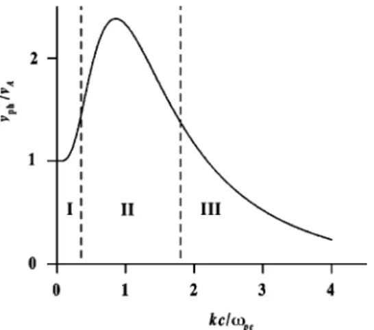
Figure 2 shows the dependence of phase velocity vph

⫽␻/k upon the wave number in the case of oblique propa-gation, cos2␪Ⰷ␮. As it was noted above, the range of wave numbers can be split into three parts corresponding to 共I兲 long waves, kⰆ␻pi/c兩cos␪兩, 共II兲 whistler waves with a

characteristic wavelength of about c/␻pe, and 共III兲

quasielectrostatic oscillations, respectively.

When considering a shock wave formation from a smooth initial disturbance of the plasma flow, we can imag-ine that a point representing the characteristic scale length of the disturbance moves along the dispersion curve shown in Fig. 2. Thereby the evolution of the disturbance resulting in

FIG. 1. The magnetic field profile for a typical supercritical quasiperpen-dicular shock wave obtained in numerical simulations 共from Ref. 24 with kind permission from Kluwer Academic兲. The foot, ramp, and overshoot are indicated.

the shock formation can be considered as a three-stage pro-cess, each stage corresponding to a particular part of the dispersion relation.

In this paper we consider the problem of the formation of oblique shocks such that cos2␪Ⰷ␮.

B. Large scale phenomena and evolution of the MHD type system

Consider a one-dimensional plasma flow such that ini-tially it is plane-polarized and consists of three regions, namely, two regions of approximately steady flow with con-siderably different velocities and the third region between the two. Suppose further that the gradients in the third region are small enough, i.e., a characteristic length of the disturbance corresponds to the region I on the dispersion curve共see Fig. 2兲, i.e., this length is much greater than the characteristic lengths related to both dispersion and dissipation. Choose a reference frame such that the only nonvanishing components of the initial disturbance of the magnetic field and plasma velocity are Bx,yand Vx,y, respectively. Such a flow is

gov-erned by the well-known equations of magnetohydrodynam-ics of an ideal medium 共see, e.g., Refs. 29, 30兲,

⳵␳ ⳵t ⫹ ⳵ ⳵x共␳Vx兲⫽0, ⳵Vx ⳵t ⫹Vx ⳵Vx ⳵x ⫽⫺ cs 2 ␳ ⳵␳ ⳵x⫺ By 4␲␳ ⳵By ⳵x , ⳵Vy ⳵t ⫹Vx ⳵Vy ⳵x ⫽ Bx 4␲␳ ⳵By ⳵x , ⳵By ⳵t ⫹Vx ⳵By ⳵x ⫽Bx ⳵Vy ⳵x ⫺By ⳵Vx ⳵x ,

where␳ is the plasma density, cs is the sound velocity, and

Bx⫽const. This is the hyperbolic quasilinear system of

equa-tions. The properties of such systems are studied in detail

共see, e.g., Refs. 29, 31兲. It is well-known that for a multitude

of initial disturbances the corresponding smooth solutions to these equations exist only during finite time intervals. At the end of such an interval a gradient catastrophe occurs, i.e.,

infinite gradients develop. Then the plasma flow overturns resulting in the formation of a multiflow region. We illustrate this phenomenon by an example of a so-called simple waves. Using a standard technique,29 we find that the magnetic field in a simple wave obeys the equation,

⳵By

⳵t ⫹Vf共By兲

⳵By

⳵x ⫽0,

which has a solution,

x⫺Vf共By兲 t⫽F共By兲, 共3兲

where F(By) is an arbitrary function of the magnetic field.

The plasma density and velocity can be easily found using the Riemann invariants, which are constant in a region occu-pied by a simple wave. Since the thermal effects do not change the qualitative features of the phenomenon, they can be neglected for simplicity. In this case the Riemann invari-ants are R1⫽ 共Bx 2_⫹B y 2_兲1/2 ␳ , 共4兲 R2⫽Vx⫾

冉

冊

冉

冊

冕

The phase velocity of the wave is given by

Vf⫽R2⫿ 3 2

冉

冊

Choose the lower signs in Eqs. 共5兲–共7兲 to consider a wave, which propagates with respect to the plasma in the positive direction of the x-axis. From Eq.共3兲 it follows that an infinite gradient of the magnetic field共as well as the gradients of the other parameters describing the plasma flow兲 develops for the first time at

t⫽minF

⬘

⬘

This gradient catastrophe could happen if the dispersion would not counteract to prevent it. These effects cannot be described by the magnetohydrodynamic equations. When characteristic lengths become shorter than c/␻_pi, one should change the model equations to take into account the disper-sion due to two-fluid nature of the plasma.

C. Dispersion effects and whistler-type precursor wave trains

If the characteristic length of the flow becomes compa-rable with the dispersion length, the system goes to the re-gion II on the dispersion curve共see Fig. 2兲, where its evolu-tion is governed by a more complicated system of the two-fluid magnetohydrodynamics.

If the initial disturbance has a small amplitude, its steep-ening will stop when the characteristic length of the region with the largest gradients attains the dispersion length

FIG. 2. The dependence of phase velocity of the oblique fast magnetosonic waves on the wave number.

c兩cos␪兩/␻pi共as it was stated above, here and in the following

we assume that the dissipation is weak, i.e., the dissipation results in the large scale variations of the plasma parameters, but it does not influence considerably the fine structure of the front兲. In this case the equations describing the evolution of the shock wave structure can be simplified by neglecting the electron inertia 共see, e.g., Refs. 1, 32兲. Thereby we obtain32

dV dt ⫽ 1 4␲␳关rot B⫻B兴, rot B⫽4␲ne c 共V⫺Ve兲, ⳵B ⳵t ⫽rot 关V⫻B兴⫺ mic e rot dV dt ⫹ mec e rot dVe dt ,

where V⫽(meVe⫹miVi)/(me⫹mi) is the bulk plasma

ve-locity, Ve,i are the fluid velocities of the electron and ion

components.

Then we can introduce two small parameters,

␧1⫽ ␤ vAl2 Ⰶ1, ␧2⫽ By⫺B0 sin␪ B0 Ⰶ1, where ␤⫽v_Ac2 _cos2_␪/2␻ pi 2 _{, l is a characteristic length of}

the disturbance, B₀is the unperturbed magnetic field,␪is the angle between the unperturbed magnetic field and the direc-tion of the wave propagadirec-tion.

Retaining the terms up to the second order with respect to these parameters, and considering only the waves propa-gating in the positive direction, after some algebra we obtain32 ⳵b ⳵t ⫹

冉

冊

where b⫽B_y⫺B₀ sin␪. This equation is equivalent to Korteweg–de Vries equation, describing nonlinear waves with a positive dispersion. It is well-known that all solutions to Korteweg–de Vries equation have no sharp crests and do not break. This means that the dispersion of short waves is strong enough to prevent the growth of gradients due to non-linear effects. However, this equation is valid only for small and smooth disturbances.

To analyze the evolution of large-amplitude distur-bances, we should at least begin with the equations of two-fluid magnetohydrodynamics, where the effects of electron inertia are also taken into account. It is generally believed that under some conditions these equations have no smooth solutions. In particular, it is well-known that stationary solu-tions can have sharp crests共see, e.g., Refs. 1, 2兲. In addition, we should expect that these equations describe also the wave breaking of the hyperbolic kind with the development of the vertical slope共a gradient catastrophe兲 and a multivalued pro-file. Up to now the rigorous proof of the corresponding math-ematical theorem has not been obtained yet. However, we can suggest several arguments confirming this statement.

From the set of equations of the two-fluid magnetohy-drodynamics, after a cumbersome but straightforward alge-bra of the reductive perturbation method33we obtain a model equation, ⳵u ⳵t ⫹u ⳵u ⳵x⫹

冕

This equation was proposed by Whitham34 as the sim-plest equation which combines two important factors, the typical hydrodynamical nonlinearity and dispersion of the arbitrary type. Indeed, the phase speed of the linear waves is given by the Fourier transform of the kernel of the integral operator,

vph共k兲⫽

冕

⫺⬁ ⫹⬁

K共x兲exp共⫺ikx兲 dx,

and vice versa,

K共x兲⫽ 1

2␲

冕

⫹⬁

vph共k兲exp共ikx兲 dk. 共10兲

Later35it was realized that the energy dissipation and pump-ing can also be described by Eq. 共9兲. Because the main goal of the paper is to study the role of the dispersion in the formation and breaking of the shock front, we neglect the dissipation in order to simplify the problem considered.

Whitham34 formulated the conjecture that Eq. 共9兲 with the kernel K_g(x) describing the dispersion of water waves,

vph共k兲⫽

冋

g

ktanh共kh0兲

册

1/2

,

where g is the gravitational acceleration and h0 is the depth

of the water, has stationary solutions with sharp crests as well as breaking nonstationary solutions. He proved that peaking of stationary solutions takes place if K(x) behaves like兩x兩⫺␣ as x→0, where␣⬎0. Since in the vicinity of the origin the normalized kernel corresponding to g⫽h0⫽1 has

the asymptotics K_g(x)⬃(2␲x)⫺1/2, the first part of the con-jecture is thereby proved. The rigorous proof of the second part requires quite ingenious arguments and was given by Naumkin and Shishmarev.35,36Moreover, they proved a more general theorem that a solution of the Whitham equation does break if the slope of the profile of an initial disturbance is sufficiently large and negative at some point and at the origin of coordinates the kernel of the integral operator has a singularity, which is weaker than兩x兩⫺␣, where 1/2⭐␣⬍3/5

共the exact statement of the theorem can be found in Ref. 35

and is also given in Appendix A兲.

It seems to be quite natural that the order of singularity of the kernel is of particular importance. Indeed, breaking as well as peaking are small scale phenomena corresponding to large wave numbers. On the other hand, it is the short-wave part of the dispersion relation that determines the behavior of the kernel in the vicinity of the coordinate origin. The Korteweg–de Vries equation 共8兲 takes vph⫽vA⫹␤k2 and

K共x兲⫽vA␦共x兲⫺␤␦

⬙

关here␦(x) is the Dirac delta-function兴 and is known to have neither peaking nor breaking solutions. In other words, the

dispersion of short waves is sufficiently strong to prevent developing infinite gradients due to nonlinearity. On the con-trary, if the kernel has no singularity at the origin and is a monotone decreasing function of兩x兩, Seliger37proved that in this case the Whitham equation does have breaking solutions

共see also Ref. 38兲. Since nonsingular integrable kernels

sat-isfy the conditions of the above-mentioned theorem proved by Naumkin and Shishmarev, this theorem should be consid-ered as a substantial generalization of the Seliger result.

Taking into account these considerations, in the follow-ing we use a simplified dispersion relation,

vph⫽

兩cos␪兩

␮1/2

兩␬兩

1⫹␬2, 共11兲 which is valid for kc/␻piⰇ1. Here vph⫽␻/kvA is the

di-mensionless phase velocity and␬⫽kc/␻peis the

dimension-less wave number. Substituting Eq. 共11兲 into Eq. 共10兲, after some straightforward calculations we obtain

K共x兲⫽⫺ 1

2␲

兩cos␪兩

␮1/2 关exp共⫺x兲Ei共x兲⫹exp共x兲Ei共⫺x兲兴,

where Ei(x) is the exponential integral. Using the asymptoti-cal expansion39

Ei共x兲⬃C⫹ln兩x兩⫹x⫹••• as x→0, we can easily obtain

K共x兲⬃⫺1

␲

兩cos␪兩

␮1/2 关C⫹ln兩x兩⫹o共x兲兴,

where C is the Euler constant. Since ln兩x兩/兩x兩⫺␣→0 as x→0 for all ␣⬎0, the condition 1 of the theorem is satisfied 共see Appendix A兲. It is easily seen that the condition 2 is also satisfied. Thus, nonlinear waves, which are described by the model Eq.共9兲 with the dispersion typical for whistler waves, do break like hyperbolic waves provided the initial distur-bance is sufficiently steep共see condition 3 of the theorem in Appendix A兲.

Although the Whitham equation with the whistler disper-sion relation is model rather than exact, it can qualitatively describe the gradient catastrophes within the front of the su-percritical nonstationary shock waves. It is worth noting that the description of this system is quite similar to that of shal-low water waves, for which similar theoretical conclusions were approved by direct experimental results.

Let us now proceed to more moderate disturbances that are not steep enough to satisfy the condition 3 of the Naumkin–Shishmarev theorem. Suppose further that in the system there exists some kind of dissipation provided by, for example, an anomalous resistivity. To take the dissipation into account, we can modify the kernel of the Whitham equa-tion共see Ref. 35 and Appendix A for details兲. In this case the disturbance can asymptotically approach some shock-like so-lution with a steady profile. Because for oblique propagation the dispersion of the fast magnetosonic wave is positive, weak shocks have a wave-train precursor damping out upstream.1,2To determine the wave number of these

oscilla-tions far upstream of the shock ‘‘ramp,’’ we should equate the upstream plasma velocity to the phase velocity given by the dispersion relation and solve the equation obtained. There exists an additional condition for a precursor to exist, namely, the group velocity should exceed the corresponding phase velocity 共see Appendix B兲. Using Eq. 共11兲 it can be easily shown that this condition is satisfied for all wave vec-tors within the range 0⭐␬⭐1. The whistler phase velocity is the highest for ␬⫽1, the corresponding Mach number is called the whistler critical Mach number17and is given by

Mw⫽

兩cos␪Bn兩

2␮1/2 .

It is well-known that the whistler precursor wave train is an essential part of the oblique subcritical shocks.1,2The very similar precursors were also evidenced for the supercritical shocks.20,21We suggest a new proof of the criteria for exis-tence of the precursor and wake wave trains 共see Appendix B兲. From this proof it is evident that these criteria are quite general, in particular, they hold not only for subcritical shock waves but for supercritical shocks as well, because a small fraction of reflected ions does not change considerably the dispersion relation for the whistler waves 共see Appendix B for more details兲.

The precursor wave train predecelerates the plasma flow upstream of the ramp of the shock and makes the contribu-tion to the energy dissipacontribu-tion. Karpman et al. suggested that this dissipation can be related to the parametric instability of the whistler waves40and/or wave-particle interaction.41If the Mach number exceeds Mw, this mechanism is switched off

and the other components of the shock front structure共e.g., the ramp兲 should provide stronger plasma flow deceleration and dissipation. This leads to the growth of gradients and as a result, the ramp of the shock is replaced by a soliton-like nonlinear whistler wave train with a characteristic wave length of about several c/␻pe. These waves were observed

within the Earth and Uranian bow shocks.10,21 Using two-fluid MHD equations, we analyze the properties of these waves in the plasma with cold ions, finite␤_e, and adiabatic equation of state for electrons 共see Appendix C兲. It was shown that the amplitude of these waves increases with Mach number and can significantly exceed the value of the magnetic field ahead of the shock. However, when Mach number exceeds the critical value Mnw, such waves do not

exist anymore. For cold plasma the corresponding Mach number, which can be referred to as a nonlinear whistler critical Mach number, is given by

Mnw⫽

兩cos␪Bn兩

共2␮兲1/2 .

As it was shown above, the critical Mach number Mnw

cor-responds also to the characteristic Mach number above which an initial disturbance resembling the quasistationary whistler wave train becomes unstable with respect to a gra-dient catastrophe, which takes place within a finite time in-terval. Thereby we come to the conclusion that M_nwcan be

taken as the estimate of the critical Mach number Mns

cor-responding to the transition between stationary and nonsta-tionary behavior of the shock front.

When Mnw is exceeded, the dispersion and dissipation

due to reflected ions and anomalous resistivity are no longer sufficient to stop the wave steepening due to nonlinear ef-fects and an additional mechanism of the energy dissipation is required. The additional dissipation can be provided by several effects accompanying the shock front nonstationarity. Indeed, a nonstationary shock should emit the whistler wave trains thereby evacuating the energy from the ramp. How-ever, when the Mach number exceeds the value,

Mgr⫽ 兩cos␪Bn兩 8

冉

冊

corresponding to the maximum group velocity of the whis-tler waves, the evacuation of the energy far upstream be-comes impossible. The short nonstationary whistler ‘‘precur-sor’’ can still exist in the foot, where the plasma flow is slightly decelerated, however, this wave train cannot propa-gate far upstream.

In the next section we present the results of full particle numerical simulations that give strong support to our state-ment that the transition from stationary to nonstationary be-havior of the shock waves takes place when the Mach num-ber becomes larger than M_nw.

Lastly, we briefly dwell upon the role of reflected ions in the shock wave structure and dynamics. It is well-known that the behavior of the reflected ions determines the large scale structure of the quasistationary supercritical shock waves and supply the major part of the dissipation required 共see, e.g., a review, Ref. 17兲. On the other hand, it is the ion dynamics that determine the time scale for quasiperiodic overturning of the high Mach number shocks. However, since the fraction of the reflected ions usually does not exceed 10%–20% for quasistationary shock waves, as a first approximation, we can neglect its contribution when deriving the criterion for transition between stationary and nonstationary shocks. In-deed, the corresponding critical Mach number is determined first of all by dispersion and nonlinearity of the fast magne-tosonic waves and these properties are predominantly deter-mined by the bulk particle populations.

FIG. 3. The stackplot for the component Bzof the

mag-netic field in the shock wave with␪Bn⫽57° and MA

III. TRANSITION FROM STATIONARITY TO NONSTATIONARITY OF THE SHOCKS: NUMERICAL SIMULATIONS

Present simulations have been performed by use of 1D fully electromagnetic relativistic particle code, where both electrons and ions are treated as particles. Standard finite-size particle techniques are used.42,43All three velocity com-ponents for all particles are taken into account but the prob-lem considered is one-dimensional, all the variables depending on x. The field components are separated into two groups, namely, the transverse components, Ey ,z and By ,z,

and longitudinal components, Ex and Bx. To find the

trans-verse components, the full set of Maxwell’s equations is solved. Longitudinal component of the magnetic field Bx is

constant and the corresponding component of the electric field obeys Poisson’s equation.

Initial and boundary conditions are similar to those al-ready described previously.22,23In short, the simulation box is separated into two adjacent parts, there is a vacuum in one of them and plasma in the another one. The latter box is bounded by reflecting walls preventing the plasma from pen-etrating into the former box. To drive a shock, a magnetic

piston is generated by applying an external current pulse in the vacuum near the boundary between the boxes.

The spatial grid is uniform. All the quantities in the code are normalized. In particular, the length is measured in the spatial grid increments a, that is, the width of the cell. In the figures in the following, shown are the normalized differ-ences between the z component of the magnetic field and its upstream value. The normalization was performed by multi-plying the differences by the factor e/me␻pe

2 _{a, where e is the}

proton charge. It is worth noting that for brevity we shall speak in the following about the magnetic field rather than the normalized difference. The ion momentum is normalized by dividing it by me␻pea. More details related to the code

can be found elsewhere.22

The present simulations are performed under the follow-ing conditions. Size of the simulation box containfollow-ing the plasma is L˜⫽8192. Initially, there are n˜e,i⫽10 particles in

each cell. The ratios of the electron and ion temperatures and masses are Te/Ti⫽1.58 and ␮⫽me/mi⫽0.005,

respec-tively. The ratio of thermal and magnetic pressures is ␤

⫽0.028.

In the simulations performed by Leroy13 it was shown

FIG. 4. The stackplot for the component Bzof the

mag-netic field in the shock wave with␪Bn⫽57° and MA

that a self-sustained shock is formed after a transitory period lasting about several ion gyroperiods calculated with the use of downstream magnetic field. In the present simulations the total run time covers about 4 ion gyroperiods calculated with the use of upstream magnetic field.

As it was noted above, there exists a close relationship between the properties of linear waves and the structure of the shock waves in plasmas.1,2 In particular, the dispersion relation influences the shape of the subcritical shock waves. In numerical modeling, a special care should be taken to avoid the distortion of the dispersion relation due to the finite-difference approximation of the equations solved.11 Because the role of whistler waves in the formation of shock wave structure is of special interest, the discretization should not distort the dispersion relation for fast magnetosonic waves with the wave numbers within the range 0⭐kc/␻pe

⭐3. Note that the phase velocity of the waves is maximum

at k⯝␻pe/c. To estimate the influence of the

finite-difference approximation on a dispersion relation, one can multiply the phase velocity by a factor sin(ka)/ka, where a is the grid increment.11,44 In the present paper we choose a

⫽c/3␻pe. The direct calculations show that these effects in

the range mentioned above can be considered as nonsignifi-cant in this case.

Two series of runs were performed, where the angle␪_Bn between the shock normal and the magnetic field upstream of the shock is equal to 57° and 80°, respectively, and Mach number varies in the wide range from about 1.6 to 8.6 in the both series. Using the simulation results, we describe the evolution of the shock wave structure as the Mach number increases.

We begin the analysis from the␪Bn⫽57° shock waves.

In this case the first critical Mach number is Mcr⬇2.54, the

linear and nonlinear whistler critical Mach numbers are Mw

⬇3.85, Mnw⬇5.45, respectively.

In the stackplot shown in Fig. 3 we observe the evolu-tion of the magnetic field profile of the supercritical shock,

MA⯝2.7. Although the shock is supercritical, the critical

Mach number is only slightly exceeded and the fraction of reflected ions, which are responsible for a typical structure of supercritical shocks, is quite small in the case considered. The quasisteady ‘‘ramp’’ is formed at the very beginning of the computational run. However, the wave train precursor expands upstream up to at least t⬎2␲/␻Bi with a higher FIG. 5. The stackplot for the component Bzof the

mag-netic field in the shock wave with␪Bn⫽57° and MA

speed than that of the shock ramp. This result is quite natural because the critical whistler Mach number is not exceeded and the stationary shock wave should have a wave train pre-cursor standing upstream of the ramp.

The next example is a quite typical supercritical shock of Alfve´n Mach number MA⯝3.3. In the stackplot for Bz

com-ponent of the magnetic field we can clearly see the formation of the ramp, overshoot, and undershoot 共see Fig. 4兲. The other characteristic feature of supercritical shocks, the foot, is also observed when analyzing the magnetic field profiles. In the foot region of the shock there is a wave train, which modulates the mean ion velocity and predecelerates the in-coming flow. It is worth noting that in the case considered both linear and nonlinear whistler critical Mach numbers are not exceeded and the shock front structure is almost station-ary.

For higher Mach numbers, MA⯝5.5 and 8.6, when both

the first critical Mach number and the nonlinear whistler Mach number are exceeded, the shock waves are nonstation-ary. For the shock wave with MA⯝5.5, stackplot is shown in

Fig. 5. Similar nonstationarity of the shock front is also evi-denced for higher Mach numbers. Figure 6 illustrates the cycle of the reformation of the magnetic field structure with the emission of the whistler wave train towards the upstream flow. During the cycle, a new ramp is formed at the forward edge of the precursor wave. Here a small-amplitude pertur-bation grows up and becomes larger than the old shock front. Now we proceed to shock waves with␪_Bn⫽80°. In this case the first critical Mach number is Mcr⬇2.74, the whistler

linear and nonlinear critical Mach numbers are Mw⬇1.23

and Mnw⬇1.74.

The stackplot in Fig. 7 shows the evolution of the mag-netic field profile for shock wave with a relatively low Mach number, MA⯝1.6. Since MA⬍Mcr, this shock is subcritical

and the fraction of reflected ions is negligible. We observe that the ‘‘ramp’’ can be considered as almost stationary for

t⬎0.2•2␲/␻Bi. Because the whistler critical Mach number

is exceeded, there is no stationary wave train upstream of the ramp. However, the maximum group velocity of whistler waves is greater than the velocity of shock wave propaga-tion, thus, a nonstationary wave precursor may be observed upstream of the ramp, at least, at the first stages of the shock formation.

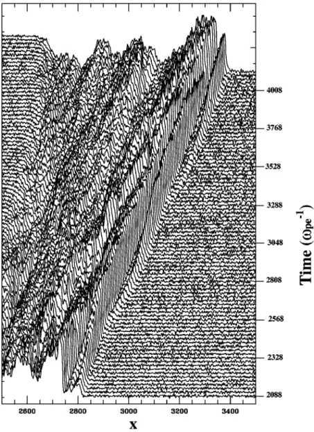
In the next example we consider the supercritical shock with MA⯝3.5. In Fig. 8 presenting the evolution of the

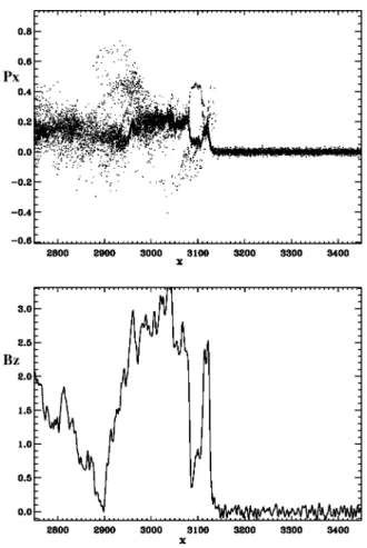
mag-netic field profile, it is easily seen that the shock is nonsta-tionary and a quasiperiodic reformation of the shock front is observed. The scenario of the reformation is essentially the same as for high Mach number shocks with␪_Bn⫽57°. At the first stage shown, the shock has a clearly defined ramp and upstream of the ramp there is a leading ‘‘wave train’’ of a small amplitude 共see also Fig. 9兲. A population of reflected ions is observed between the ramp and the peak of the lead-ing wave train共see the ion phase space display in Fig. 9兲. In this case the whistler precursor consists of only one peak

FIG. 6. The magnetic field profiles for a shock wave with␪Bn⫽57° and

MA⫽5.5 at 共a兲 t⫽2496␻pe⫺1,共b兲 t⫽2808␻pe⫺1,共c兲 t⫽3096␻pe⫺1, and共d兲

because in the simulation the whistler phase velocity along the magnetic field has the same order of magnitude as the thermal speed of electrons, so that the damping of the whis-tlers is considerable. The amplitude of the leading wave train is gradually increasing. At some time a new population of reflected ions appears upstream of the precursor 共see Fig. 10兲. When its amplitude becomes comparable with that of the ramp and, finally, exceeds it, thereby a new ramp and a new precursor are formed 共see Figs. 11 and 12兲. The pro-cesses described are repeated quasiperiodically.

Finally, the results of the simulations for both chosen values of␪Bn confirm our statement that the transition from

stationary to nonstationary behavior of the quasiperpendicu-lar shock occurs when nonlinear whistler critical Mach num-ber is exceeded.

IV. CONCLUSION

In the present paper we study the problem of the nonsta-tionarity of quasiperpendicular high Mach number shocks. Previously, Kennel et al.17 introduced a critical Mach num-ber Mns above which shock waves become nonstationary.

However, up to now the estimates of Mns were not

sug-gested. In the present paper, Mns is determined for oblique

quasiperpendicular fast magnetosonic shock waves.

Theoretical analysis and experiments show that the whistler waves are an intrinsic feature of the oblique colli-sionless shock waves. For supercritical shock waves, the ramp region, where an abrupt increase of the magnetic field occurs, can be treated as a nonlinear whistler wave of large amplitude. In addition, oblique shock waves can possess a linear whistler precursor. There exist two critical Mach num-bers related to the whistler components of the shock wave, the first is known as a whistler critical Mach number intro-duced by Kennel et al.,17 Mw, and the second can be

re-ferred to as a nonlinear whistler critical Mach number, M_nw. It is worth noting that Mw⬍Mnw. When the whistler critical

Much number is exceeded, a stationary linear wave train cannot stand ahead of the ramp. Above the nonlinear whistler critical Mach number, the stationary nonlinear wave train cannot exist anymore within the shock front. In this case the dispersion cannot prevent steepening of the shock front due to nonlinear effects and a gradient catastrophe occurs. As a result, the shock wave becomes nonstationary. Using model

FIG. 7. The stackplot for the component Bzof the

mag-netic field in the shock wave with␪Bn⫽80° and MA

equation description, we carried out the analysis of the dy-namics of oblique shock waves and found that this equation does describe the wave breaking of the hyperbolic kind with the development of the vertical slope and a multivalued pro-file.

To obtain the ␤- and ␪Bn-dependencies of Mnw

corre-sponding to the transition between the stationary and nonsta-tionary behavior of the shock wave, in the framework of the two-fluid magnetohydrodynamics we study the structure of nonlinear whistlers in plasmas with finite electron beta and adiabatic equation of state 共see Appendix C兲.

In accordance with the results of the theoretical analysis, numerical simulations making use of the 1D full particle electromagnetic code demonstrated that the transition to the nonstationarity is always accompanied by the disappearance of the stationary whistler wave train within the shock front, i.e., the nonlinear whistler critical Mach number Mnw is

closely related to Mns. The simulations show that front of

the high Mach number shocks overturns quasiperiodically and the dynamics of the whistler wave trains within the front are of particular importance as was supposed previously.11,20 Recent experimental observations45 of the nonstationary

whistler waves in the vicinity of the Earth bow shock con-firm this model of the shock front nonstationarity.

In addition, we suggested a new proof of the criteria for small-amplitude linear precursor or wake wave trains to exist

共see Appendix B兲. It was also shown that these criteria are

quite universal and can be considered as necessary and suf-ficient conditions that turn out to be independent on both the nature of the waves and dissipative effects provided the me-dium far ahead and far behind the shock is stable and the dissipation is weak enough for weakly damping waves to exist.

ACKNOWLEDGMENTS

The authors would like to acknowledge the International Space Science Institute 共Bern, Switzerland兲 for the financial support and the welcome of the working group ‘‘Multi-dimensional aspects of particle dynamics through the Earth’s collisionless shock.’’ V.V.L. is grateful to the administration of the Region Centre of France for financial support during his stay at LPCE 共Orle´ans, France兲. He also acknowledges the warm hospitality of LPCE.

FIG. 8. The stackplot for the component Bzof the

mag-netic field in the shock wave with␪Bn⫽80° and MA

All present numerical simulations have been performed on supercomputers of IDRIS center共Orsay, France兲.

APPENDIX A: GRADIENT CATASTROPHE FOR THE WHITHAM EQUATION

Consider the Whitham equation,

⳵u

⳵t ⫹u

⳵u

⳵x⫹Ku⫽0,

whereK is a linear pseudodifferential operator. This operator can be written in two forms,

Ku⫽

冕

冕

冕

and Kˆ is called a symbol of the operatorK. Let Kˆ1⫽R(Kˆ) and Kˆ2_{⫽I(Kˆ). If only real solutions to the Whitham}

equa-tion are considered, Kˆ1and Kˆ2are called the dissipative and conservative parts of the symbol Kˆ , respectively.

For the Whitham equation Naumkin et al.35 proved the following:

Theorem: Suppose that

共1兲 the kernel K(x) satisfies the conditions

K共x兲苸C1共R1\0兲艚L1共R1兲, 兩K共x兲兩⭐c兩x兩⫺␣,

兩K

⬘

冕

⬘

where

␣⫽3/5⫺␥, ␥苸共0,1/10兴, c⬎0, a苸共0,1兴;

共2兲 the integral operator is dissipative, i.e., the symbol of the

operator satisfies the inequality

Kˆ1共p兲⭓0 for 兩k兩⭓h⬎0;

共3兲 the initial perturbation u¯(x) belongs to the Sobolev space

H⬁(R1) and has a sufficiently large steepness m0

⫽兩minx苸R₁¯u

⬘

冑

冉

冊

FIG. 9. The magnetic field profile共bottom panel兲 and Px– x phase space

共top panel兲 for a shock wave with␪Bn⫽80° and MA⫽3.5 at t⫽2860␻pe⫺1.

FIG. 10. The magnetic field profile共bottom panel兲 and Px– x phase space

b⫽ sup 兩k兩⭐h共0,⫺Kˆ 1_{共k兲兲, u} 1⫽ max x苸R₁ 兩u¯

⬘

冕

冉

冊

Then there exists a solution u(t,x)

苸C⬁_(关0,T

0);H⬁(R1)) breaking at the moment of time T0.

The following two-sided inequalities hold for T₀:

m0⫺1共1⫹␥兲⫺1⭐T0⭐m0⫺1共1⫺␥兲⫺2.

APPENDIX B: PRECURSORS AND WAKES

Suppose that the dissipation is negligible and the waves considered have a dispersion relation ␻⫽␻(k). Then the phase and group velocities are

vph⫽ ␻

k, vgr⫽

⳵␻ ⳵k,

respectively. When considering a precursor 共wake兲, suppose further that the velocity of the plasma far ahead共behind兲 the shock is U1,2in the frame where the shock is at rest. Then a

steady precursor 共wake兲 wave train can stand in the flow provided there exists a wave number k0 such that

␻ k

冏

冏

冏

for a precursor and

⳵␻ ⳵k

冏

冏

for a wake. The condition共B1兲 is trivial—the phase velocity of the waves considered equals the velocity U0 of the flow.

The second criterion 共B2兲 also becomes obvious if we con-sider a formation of a shock wave from a discontinuity sat-isfying the Rankine–Hugoniot conditions and to this end choose a reference frame where the shock is stationary. When emitting the waves both upstream and downstream, this step-like disturbance will be transformed into a steady shock with a precursor and/or wake wave trains. Since the wave number like the energy of the waves is transferred with the corresponding group velocity 共see, e.g., Ref. 34兲, the waves can penetrate upstream and form a precursor if their group velocity exceeds the flow velocity ahead of the shock. To be convected downstream thereby forming a wake, the waves should have the group velocity which is less than that of the flow behind the shock.

It appears that criteria for a steady wave train precursor or wake of the shock wave to exist were developed for the

FIG. 11. The magnetic field profile共bottom panel兲 and Px– x phase space

共top panel兲 for a shock wave with␪Bn⫽80° and MA⫽3.5 at t⫽3624␻pe⫺1.

FIG. 12. The magnetic field profile共bottom panel兲 and Px– x phase space

first time by Tidman et al.46To prove the criteria, they con-sider a model shock wave, which was represented by an infinite plane discontinuity, and a model dispersion relation in the form,

D共␻,k兲⫽

兿

i 关␻⫺␻i共k兲⫹i␧兴,

where a small positive␧ describes a weak dissipative effects. They suppose that the electric current within the shock tran-sition oscillates periodically, and using the linearized Vlasov–Maxwell equations, calculate the electromagnetic field generated by this current. The relationships obtained are rather cumbersome, but the above mentioned criteria follow from them immediately. Perez et al.47 carried these calcula-tions further using the exact dispersion relation for a cold plasma.

As was shown above, the criteria共B1兲 and 共B2兲 are easy to understand from the physical point of view and can be considered as necessary conditions for a precursor and/or wake to exist for shock waves in a plasma as well as in other media. However, the question remains as to the correspond-ing sufficient conditions. Indeed, uscorrespond-ing a stationary point analysis ahead and behind the shock waves in the dissipative magnetohydrodynamics, Coroniti48showed that the different dissipative effects 共resistivity, thermoconductivity, and vis-cosity兲 are not equivalent in the formation of the shock waves, e.g., the viscosity alone cannot form a fast MHD shock wave but the resistivity can. On the other hand, the criteria 共B1兲 and 共B2兲 does not contain any information about dissipation. One can suggest the two possibilities. First, these criteria are universal and sufficient for a precur-sor 共wake兲 to exist upstream 共downstream兲 the dispersive shock wave no matter what kind of waves is considered and what kind of dissipation is significant. Second, these criteria are only necessary and in each case Eq. 共B2兲 should be re-placed by a more strong condition, which is characteristic for a particular kind of the waves and/or dissipation. It can be easily shown that valid is the first statement.

To begin with, suppose that all parameters describing a wave depend upon time and coordinates like f⫽ f0

⫻exp(⫺i␻t⫹ikx) and the dispersion relation for these waves

is

D共␻,k兲⫽0. 共B3兲 If the dissipation is present but weak for the waves consid-ered, Eq.共B3兲 can be written approximately as

D0共␻,k兲⫹D1共␻,k兲⫽0, 共B4兲

where D0(␻,k) is a function which determines the

disper-sion relation ␻⫽␻0(k) when the dissipation is absent and

the dissipation is responsible for the second term D1(␻,k)

the absolute value of which is much smaller than that of the first term. For plasma waves, the term D0(␻,k) is

deter-mined by the Hermitian part of the dielectric tensor and the term D1(␻,k) depends on both Hermitian and

anti-Hermitian parts of the tensor 共see, e.g., Ref. 27兲. Equation

共B4兲 can be solved by means of a perturbation method. At

the first step, the dissipation is neglected, and from the

equa-tion D₀(␻,k)⫽0 we obtain an approximate dispersion rela-tion␻⫽␻₀(k) giving the real part␻₀of the wave frequency,

␻⫽␻0⫹i␥, 共B5兲

where ␥ is the increment. Substituting Eq. 共B5兲 into Eq.

共B4兲, in the next approximation the increment is obtained,

␥⫽⫺ D1 ⳵D₀/⳵␻

冏

(␻₀(k), k)

. 共B6兲

If medium is in a stable state as we suppose to be the case far ahead and far behind the shock, all disturbances should damp,␥⬍0. Hence,

D1 ⳵D₀/⳵␻

冏

(␻₀(k), k)

⬎0.

Suppose that in the reference frame, where the unper-turbed plasma is at rest, the shock wave is moving along the

x axis in the positive direction. Then in the shock frame both

the precursor and wake are stationary,␻⫽0, and the velocity of the medium upstream and downstream of the shock is negative, U1,2⬍0. Using the formulas for the nonrelativistic

Doppler effect, we find that in the reference frame, where the medium upstream or downstream is at rest, the precursor and wake waves have real frequencies,

␻⫽kU1,2, 共B7兲

respectively, but the corresponding wave numbers will be complex, k⫽k0⫹i␬, where ␬ is an imaginary part of the

wave number. Substituting Eq.共B7兲 into the dispersion rela-tion 共B4兲 and making use of the technique utilized above when finding the increment, we obtain

␬⫽ D1 U1,2 ⳵D0 ⳵␻ ⫺ ⳵D0 ⳵k

冏

Using Eq.共B6兲 and the definition of the group velocity, this relationship can be rewritten as

␬⫽ ␥

vgr⫺vph

冏

.

If the group velocity exceeds the velocity of the flow, we see that ␬⬎0 and the amplitude of the waves will vanish as x

→⫹⬁ as should be the case for the precursor. For the wake

wave trains, which vanish as x→⫺⬁, the opposite condition should hold. The criteria共B2兲 are thereby proved.

Finally, it is worth noting that the well-known criteria for existence of the precursor and wake wave trains in the vicin-ity of a dispersive shock are quite universal and can be con-sidered as necessary and sufficient conditions that turn out to be independent on both the nature of the waves and dissipa-tive effects provided the medium far ahead and far behind the shock is stable and the dissipation is weak enough for weakly damping waves to exist.

APPENDIX C: NONLINEAR WHISTLER WAVES IN A PLASMA WITH HOT ELECTRONS

Oblique nonlinear whistler waves in a cold plasma were studied for the first time by Kazantsev.49If ions are cold and electrons are ‘‘warm’’ and isothermal, the similar problem was solved by Kakutani et al.50 In this appendix, we extend these results for electrons with an adiabatic equation of state. For one-dimensional flows, the two-fluid MHD equa-tions can be written as follows:

⳵n ⳵t⫹ ⳵ ⳵x共nVx兲⫽0, 共C1兲 ⳵Vx ⳵t ⫹Vx ⳵Vx ⳵x ⫽ e 共me⫹mi兲c 关共 Viy⫺Vey兲Bz⫺共Viz⫺Vez兲By兴 ⫺ 1 n共me⫹mi兲 ⳵p ⳵x, 共C2兲 ⳵V˜i ⳵t ⫹Vx ⳵V˜i ⳵x ⫽ e mi E ˜_⫹i e mic共Vx B ˜_⫺V˜ iBx兲, 共C3兲 ⳵V˜e ⳵t ⫹Vx ⳵V˜e ⳵x ⫽⫺ e m_eE˜⫺i e m_ec共VxB˜⫺V˜eBx兲, 共C4兲 1 c ⳵E˜ ⳵t ⫽i ⳵B˜ ⳵x⫺ 4␲ne c 共V˜i⫺V˜e兲, 共C5兲 1 c ⳵B˜ ⳵t ⫽⫺i ⳵E˜ ⳵x, 共C6兲 B_x⫽B₀ cos␪⫽const, 共C7兲 ⳵p ⳵t⫹Vx ⳵p ⳵x⫹␥p ⳵Vx ⳵x ⫽0, 共C8兲

where␥ is the specific heat ratio for electron component. We assume that quasineutrality holds and for both electrons and ions n denote the number density. The x-components of the fluid velocity of electrons and ions are approximately equal and denoted by Vx. For brevity, we introduce the following

complex parameters: transverse electric field E˜⫽Ey⫹iEz,

transverse magnetic field B˜⫽By⫹iBz, and transverse fluid

velocities V˜⫽V_y⫹iV_z of electron and ion components. In addition to the continuity Eq.共C1兲, the system 共C1兲–

共C8兲 has the following conservation relations for momentum

and energy: ⳵ ⳵t

冋

册

冋

册

冋

册

冋

册

再

冋

册

冎

再

冋

册

冎

For a stationary solution, we can choose a reference frame such that the time derivatives vanish. Then from Max-well equations it follows that E˜⫽const and we can let Ey

⫽0. Assume further that at infinity the plasma is

undis-turbed. Here we can let V˜e,i⫽0. Then electric and magnetic

field components are

Bx⫽B0 cos␪, By⫽B0 sin␪, Bz⫽0,

Ey⬅0, Ez⬅⫺

Vx0

c B0 sin␪,

respectively. For definiteness, in the following we assume that ␥⫽2.

After some straightforward algebra we can easily obtain

y2⫹z2⫽sin2 ␪⫹2M_A2共1⫺v兲⫹␤

冉

v2

冊

y

⬙

⬘

共C10兲

z

⬙

⬘

where y⫽By/B0 and z⫽Bz/B0 are the dimensionless

mag-netic field components, MA is the Alfve´n Mach number, ␤

⫽8␲p0/B0

2_{, ⍀⫽(␮}1/2_⫹␮⫺1/2_{)cos␪, and}

v is the

x-component of the dimensionless plasma velocity

normal-ized to its unperturbed value at infinity. The primes denote the derivatives with respect to the dimensionless coordinate introduced by

d␰⫽ eB0

共memi兲1/2vc

dx.

At infinity we havev⫽1, y⫽sin␪, z⫽0, and first and sec-ond derivatives of the magnetic field vanish. Equations

共C10兲–共C11兲 can be written in the following form:

y

⬙

⬘

⬙

⬘

2_⫺cos2 _{␪兲y sin ␪, 共C14兲}

and r2⫽y2⫹z2. It is convenient to write the addend␺(r) in terms of the plasma velocity,