HAL Id: hal-00299506
https://hal.archives-ouvertes.fr/hal-00299506
Submitted on 2 Apr 2008
HAL is a multi-disciplinary open access
archive for the deposit and dissemination of
sci-entific research documents, whether they are
pub-lished or not. The documents may come from
teaching and research institutions in France or
abroad, or from public or private research centers.
L’archive ouverte pluridisciplinaire HAL, est
destinée au dépôt et à la diffusion de documents
scientifiques de niveau recherche, publiés ou non,
émanant des établissements d’enseignement et de
recherche français ou étrangers, des laboratoires
publics ou privés.
upper Rhine catchment
S. Jaun, B. Ahrens, A. Walser, T. Ewen, C. Schär
To cite this version:
S. Jaun, B. Ahrens, A. Walser, T. Ewen, C. Schär. A probabilistic view on the August 2005 floods in
the upper Rhine catchment. Natural Hazards and Earth System Science, Copernicus Publications on
behalf of the European Geosciences Union, 2008, 8 (2), pp.281-291. �hal-00299506�
www.nat-hazards-earth-syst-sci.net/8/281/2008/ © Author(s) 2008. This work is licensed under a Creative Commons License.
and Earth
System Sciences
A probabilistic view on the August 2005 floods in the upper Rhine
catchment
S. Jaun1, B. Ahrens2, A. Walser3, T. Ewen1, and C. Sch¨ar1
1Institute for Atmospheric and Climate Science, ETH Zurich, Switzerland
2Institute for Atmosphere and Environment, Goethe-University Frankfurt a.M., Germany 3MeteoSwiss, Zurich, Switzerland
Received: 24 October 2007 – Revised: 21 February 2008 – Accepted: 5 March 2008 – Published: 2 April 2008
Abstract. Appropriate precautions in the case of flood
occur-rence often require long lead times (several days) in hydro-logical forecasting. This in turn implies large uncertainties that are mainly inherited from the meteorological precipita-tion forecast. Here we present a case study of the extreme flood event of August 2005 in the Swiss part of the Rhine catchment (total area 34 550 km2). This event caused tremen-dous damage and was associated with precipitation amounts and flood peaks with return periods beyond 10 to 100 years. To deal with the underlying intrinsic predictability limita-tions, a probabilistic forecasting system is tested, which is based on a hydrological-meteorological ensemble prediction system. The meteorological component of the system is the operational limited-area COSMO-LEPS that downscales the ECMWF ensemble prediction system to a horizontal reso-lution of 10 km, while the hydrological component is based on the semi-distributed hydrological model PREVAH with a spatial resolution of 500 m. We document the setup of the coupled system and assess its performance for the flood event under consideration.
We show that the probabilistic meteorological-hydrological ensemble prediction chain is quite effective and provides additional guidance for extreme event forecasting, in comparison to a purely deterministic forecasting system. For the case studied, it is also shown that most of the benefits of the probabilistic approach may be realized with a comparatively small ensemble size of 10 members.
Correspondence to: S. Jaun
(simon.jaun@env.ethz.ch)
1 Introduction
During the period from 19 to 23 August 2005, Switzerland and neighbouring countries were hit by a heavy precipita-tion event. Because of a predisposed hydrological situaprecipita-tion, the soils were already saturated and could not absorb the additional intense rainfall of up to 300 mm within 48 h (cf. Fig. 1). As a consequence, the water levels in rivers and lakes rose dramatically, causing flooding in many regions. In areas with steep terrain, landslides and mudflows occured and many people had to be evacuated. Several fatalities re-sulted and the total financial losses reached approximately 3 billion Swiss Francs (MeteoSchweiz, 2006; Bezzola and Hegg, 2007).
In order to plan appropriate measures to mitigate the ef-fects of such extreme precipitation events, hydrological fore-casts with long lead times (>24 h) are needed. For the horizontal scales considered, such forecasts are only pos-sible with the use of coupled hydrometeorological models, driven by quantitative precipitation forecasts (QPF). Long lead times are accompanied by larger uncertainties, espe-cially for meteorological forecasts. As it would be impru-dent to simply ignore these uncertainties (Pappenberger and Beven, 2006), probabilistic forecasts can be applied. Prob-abilistic forecasts in terms of ensemble forecasts are estab-lished for operational meteorological forecasts and are now more frequently used for hydrological problems (e.g. Pap-penberger et al., 2005; Roulin and Vannitsem, 2005; Siccardi et al., 2005; Rousset et al., 2007; Komma et al., 2007; Ver-bunt et al., 2007).
In general, the output uncertainty of a hydrological model is affected by several components. The main sources of uncertainty consist of the initialization uncertainty (i.e. the
Fig. 1. Estimates of observed precipitation [mm] for 21–22 August
derived from radar and rain gauge data (Figure: C. Frei, published in MeteoSchweiz (2006)). C1 C2 C3 C4 C5 C6 C7 C8 C9 C10 C11 C12 C13 C14 C15 C16 C17 C18 C19 C20 C21 C22 C23 N 100 km
Fig. 2. Catchment overview, showing the defined catchments with
respective identifier (C1, ..., C23) upstream of the Rheinfelden gauge (cf. Table 1).
initial state of the model), the model uncertainty (uncertainty from parameters and the conceptualization) and the input un-certainty (unun-certainty from the meteorological data used to drive the model) (Vrugt et al., 2005). In this work, the main focus will be on the input uncertainty, as forecasted meteo-rological data is regarded as the most uncertain component (Todini, 2004).
Meteorological ensemble prediction systems (EPSs) are operationally available at the global scale from, e.g. the US National Center for Environmental Predictions (NCEP, Toth and Kalnay, 1997), the European Centre for Medium Range Weather Forecasts (ECMWF, Molteni et al., 1996) and the Meteorological Center of Canada (MSC, Houtekamer et al., 1996). The spread of the ensemble members represents mainly the initialization uncertainty of the meteorological model, which is considered as the main source of uncertainty for large scale atmospheric patterns in forecasts up to 3–5 days (Buizza, 2003). As these large scale numerical
mod-Table 1. Catchment identifiers with names of the respective rivers
and gauges as well as the size of the catchments.
identifier river gauge size [km2]
C1 Hinterrhein Furstenau 1575
C2 Vorderrhein Ilanz 776
C3 Rhine Domat-Ems 3229
C4 Landquart Felsenbach 616
C5 Ill Gisingen (A) 1281
C6 Rhine Diepoldsau 6119 C7 Rhine Neuhausen 11 887 C8 Thur Andelfingen 1696 C9 Rhine Rekingen 14 718 C10 Aare Ringgenberg 1129 C11 Aare Thun 2490 C12 Aare Hagneck 5128 C13 Aare Brugg-Agerten 8217 C14 Emme Wiler 939 C15 Aare Brugg 11 750 C16 Linth Weesen 1061 C17 Limmat Zurich 2176 C18 Limmat Baden 2396 C19 Reuss Seedorf 832 C20 Reuss Luzern 2251 C21 Reuss Mellingen 3382 C22 Aare Untersiggenthal 17 625 C23 Rhine Rheinfelden 34 550
els are not accurate at modeling local weather, because local sub-grid scale features and dynamics are not resolved, dy-namical downscaling methods are applied by use of a limited area model (e.g. COSMO-LEPS, nested into the ECMWF ensemble, described in the following section). In terms of computational time, a dynamical downscaling is expensive and thus it is not feasible to downscale the full global ensem-ble for everyday operational applications. Therefore the en-sembles are normally reduced and only a subset of its mem-bers is used.
In an earlier study, the effect of this reduction of ensemble size on spread was investigated for a coupled meteorological-hydrological ensemble system (Verbunt et al., 2007). Here, we investigate the reprensentativeness of the reduced ensem-ble by means of quantitative statistics and discuss proensem-blems associated with its interpretation. This complementary ap-proach was chosen in order to analyse all the information contained in the ensemble, as spread alone indicates only the expected uncertainty of the forecast, and not its actual skill. This is an important question with regard to the usability of a probability forecast during an extreme event.
This paper investigates the benefit of using a coupled meteorological-hydrological ensemble approach for extreme flood forecasting, using the August 2005 event as a case study. In addition to selected gauges, the full extent of the study area is considered, which consists of the upper Rhine
basin down to the gauge Rheinfelden, encompassing an over-all area of 34 550 km2. To account for inhomogeneities in topography, atmospheric processes and runoff regimes, the domain is further divided into 23 subcatchments (cf. Fig. 2), based on the setup described in Verbunt et al. (2006).
2 Methods
2.1 Deterministic forecasting system
The deterministic hydrological forecasts were driven by the operational weather forecast model aLMo (recently renamed to COSMO-7). This model is the MeteoSwiss implemen-tation of the COSMO model (Consortium for Small-scale Modeling, Steppeler et al., 2003), using a horizontal grid-spacing of 0.0625 degrees (7 km) and 45 model levels. Six meteorological surface variables (temperature, precipitation, humidity, wind, sunshine duration derived from cloud cover, global radiation) are downscaled to 500 m grid-spacing (bi-linear interpolation, temperature adjusted according to ele-vation by adopting a constant lapse rate of 0.65◦C/100 m), to meet the grid size requirements of the hydrological model.
The semi-distributed hydrological model PREVAH (Vivi-roli et al., 2007) is then applied with hourly time steps, re-sulting in a deterministic 72 h hydrological forecast (sub-sequently referred to as HALMO). PREVAH (Preciptation Runoff EVApotranspiration Hydrotope) uses hydrologic re-sponse units (HRUs, Fl¨ugel, 1997) and the runoff genera-tion module is based on the concepgenera-tion of the HBV-model (Bergstr¨om and Forsman, 1973; Lindstr¨om et al., 1997), adapted to a spatially distributed application. Further infor-mation on the model physics, structure, interpolation meth-ods and parameterisations can be found in Gurtz et al. (1999), Gurtz et al. (2003) and Zappa (2002). The initial conditions of the hydrological model are obtained from a continuous reference simulation driven by meteorological observations (HREF).
2.2 Ensemble prediction system
The meteorological ensembles originate from the operational global atmospheric EPS of ECMWF with 51 members. The global atmospheric model is run with a horizontal resolution of T255 (equivalent to about 80×80 km2) using 40 vertical model levels. The generation of the ensemble is based on singular vectors to create optimally perturbed initial states (Buizza and Palmer, 1995). This information is downscaled by the limited-area EPS COSMO-LEPS (Marsigli et al., 2005; Montani et al., 2003). Due to computational con-straints, the operational COSMO-LEPS refines a subsample of 10 representative ensemble members, selected by a clus-ter analysis (Molteni et al., 2001). Prior to the clusclus-tering analysis, the preceding EPS simulation from the previous day is combined with the actual forecast. Hence the clus-tering is applied to a recombined ensemble consisting of 102
members. This procedure, using ’old’ forecast information, generally results in a widening of spread of the reduced en-semble. The clustering identifies similar circulation patterns based on the analysis of wind, geopotential and humidity on three pressure levels (500 hPa, 700 hPa, 850 hPa) for two lead times (96 h, 120 h).
From the resulting 10 clusters, the respective represen-tative cluster members (RM) are selected and dynamically downscaled over a domain covering central and southern Eu-rope. These ensemble members are run on a rotated spherical grid with a horizontal grid-spacing of 0.09◦×0.09◦, equiv-alent to about 10×10 km2, and 32 model levels (LEPS10). They are run up to 132 h with a three-hourly output interval. The resulting high-resolution meteorological ensemble forces a hydrological ensemble prediction system (HEPS10). The treatment of the meteorological variables is analogous to the treatment of the aLMo variables. The cluster sizes can optionally be used to weight the RMs of HEPS10 (HEPS10w). No additional perturbations were realised at the level of the hydrological model, e.g. for consideration of ini-tialization uncertainties.
For the period of the case study considered and in distinc-tion to the operadistinc-tional COSMO-LEPS, the full 51-member EPS was downscaled by using the LEPS methodology, nest-ing the COSMO model on each EPS member. The resultnest-ing full ensemble (HEPS51) will be used to assess the potential loss in forecast skill associated with the reduction of the en-semble size through cluster techniques.
2.3 Set-up of simulations
For the quantitative analysis we focus upon a 60-h time win-dow (cf. Fig. 3) covering the event period (21 August 2005, 12:00 UTC – 23 August 2005, 24:00 UTC). Forecast perfor-mance will be assessed for three different overlapping fore-cast periods, with forefore-casts initialized at 00:00 UTC on 19, 20 and 21 August (corresponding to maximum lead times of 120 h, 96 h, 72 h, respectively). For each of these forecast periods consideration is given to the HALMO, HEPS10 and HEPS51 forecasts.
The meteorological EPS forecasts are initialized at 12:00 UTC and span 132 h. The first 12 h are not considered for the hydrological coupling, resulting in a forecast range of 120 h. This cutoff considers the temporal availability of the operational forecasts.
As the forecast of HALMO only spans 72 h, it was ex-tended to the 120 h forecast range of HEPS10 and HEPS51 by using persistence for all meteorological variables, except precipitation, which was set to zero. This is justified for the HALMO simulation starting on 20 August, as the forecast range contains most of the precipitation leading to the event, but bears some simplification for the HALMO simulation starting on 19 August.
H EPS H AL MO 1 9 .8 .0 5 2 0 .8 .0 5 2 1 .8 .0 5 2 2 .8 .0 5 2 3 .8 .0 5 2 4 .8 .0 5 2 5 .8 .0 5
Fig. 3. Defined event period (red, 21 August 2005 12:00 UTC – 23
August 2005 24:00 UTC) with overlapping simulation ranges. The bars indicate the forecast periods of the ensembles (HEPS, 120 h) and the deterministic run (HALMO, 72 h). The dashed lines indi-cate the extension of the deterministic simulations to 120 h (see text for details).
2.4 Validation methodology
Event discharges were estimated for the defined event period of 60 h, in order to assess the representation of runoff vol-umes by the model chain.
Exceedance probabilities were calculated for the afore-mentioned 60-h time window (cf. Fig. 3) for an event size corresponding to a 10 year recurrence period. For each of the 23 catchments considered, the corresponding discharge thresholds were taken from estimates of the Swiss Federal Office for the Environment (published on the internet, see http://www.bafu.admin.ch/hydrologie). This analysis targets the occurrence of flood peaks, but does not assess the timing of the forecast.
To perform a probabilistic verification of the time series within the time window considered, we use the Brier skill score (BSS) described in Wilks (2006). This score is widely used for the evaluation of probabilistic forecasts in meteoro-logical sciences (e.g. Nurmi, 2003). In deterministic hydro-logical applications, the Nash-Sutcliffe coefficient (E, Nash and Sutcliffe, 1970) is widely used for evaluation purposes (Legates and McCabe, 1999; Ahrens, 2003). By briefly in-troducing both scores (BSS and E), it will be demonstrated that the BSS can be regarded as a probabilistic analogue of E.
The usual formulation of E is given by E = 1 − Pn t =1(ot−yt)2 Pn t =1(ot − ¯o)2 =1 − MSE MSEref . (1)
Here yt and ot denote the forecasted and observed time se-ries, respectively, and ¯othe mean of the observations over the forecast period. The right-hand side of Eq. (1) shows that E may be interpreted as the skill score associated with the mean squared error (MSE). As any skill score, it measures the im-provement of a forecast relative to a reference forecast (here
taken as a forecast of the correct mean discharge ¯o). This is consistent with the interpretation of E as the coefficient of determination (representing the fraction of variability in ot that is contained in yt).
The BSS is based on the Brier score (BS) where BS = 1 n n X t =1 (pyt−pot)2. (2)
It represents the mean squared error of the probability fore-cast, where pytdenotes the forecasted probability for the oc-currence of the event, and pot describes the observation at the corresponding time step t (with n denoting the number of time steps). If the event is observed (not observed) at time t, we have pot=1 (pot=0). The BS is bounded by zero and one. While a perfect forecast would result in BS=0, less ac-curate forecasts receive higher sores. A comparison of the BS against the mean squared error (MSE) shows the anal-ogy between the two measures. The two scores only differ in that the squared differences are taken from the effective value of the forecasted variable in the case of the MSE, while for the BS they are taken from the forecast probabilities and the subsequent binary observations (Wilks, 2006). The BSS is finally obtained by relating the BS of the forecast to the BS of a reference forecast according to
BSS = 1 − BS
BSref. (3)
The BSS can take values in the range −∞≤BSS≤1. Whereas BSS>0 indicates an improvement over the refer-ence forecast, a forecast with BSS≤0 lacks skill with respect to the reference forecast.
In meteorological applications, the reference forecast is usually taken as the climatological event frequency. Here in-stead we use the observed event frequency as reference, i.e. BSref= 1 n n X t =1 ( ¯po − pot)2, (4)
where ¯po denotes the frequency of observed occurrence of the event in the n time steps considered. Comparing Eq. (3) and Eq. (4) with Eq. (1), an analogy between BSS and E (consistent with the above argumentation regarding BS and MSE) emerges and E can be interpreted in the same way as BSS for probabilistic forecasts. E can take values in the range −∞≤E≤1, with E>0 indicating an improvement over fore-casting the observed event mean, while E≤0 shows no ad-ditional skill. As a consequence, BSS as defined above, can be regarded as the probabilistic representation of E. We use the observed event frequency during the respective forecast period for three main reasons: (a) to resolve the temporal evolution of the runoff peak also for catchments not reaching extreme runoff values (catchment and event specific thresh-olds), (b) to circumvent the sometimes uncertain statistics of recurrence period calculations for extreme events and (c) to
(a) (b) 0 20 40 60 80 100 120 0 .5 1 .0 1 .5 2 .0 2 .5 hours ru n o ff [ mm/ h ] HQ2 HQ20 HQ200 runoff measured runoff HREF runoff HALMO runoff HEPS10 runoff HEPS51 HEPS10w median HEPS51 median HEPS10w IQR HEPS51 IQR 5 2 .5 0 p re ci p it a ti o n [ mm/ h ] 0 20 40 60 80 100 120 0 .5 1 .0 1 .5 2 .0 hours ru n o ff [ mm/ h ] HQ2 HQ20 HQ200 runoff measured runoff HREF runoff HALMO runoff HEPS10 runoff HEPS51 HEPS10w median HEPS51 median HEPS10w IQR HEPS51 IQR 5 2 .5 0 p re ci p it a ti o n [ mm/ h ]
Fig. 4. Hydrological hindcasts, starting on 20 August for gauge (a) Hagneck (C12, 5170 km2) and (b) Mellingen (C21, 3420 km2) in the Aare and the Reuss watersheds. HEPS10w (red) is shown with corresponding IQR and median, the same for HEPS51 (blue). The varying thickness of the red lines corresponds to the weight of the respective RM. Additionally, the deterministic run HALMO (black), measured runoff (dark blue) and the reference simulation HREF (green) are shown. Spatially interpolated observed precipitation (catchment mean) is plotted from the top.
gain the possibility to directly compare the validation of fore-casted runoff to the validation of forefore-casted areal precipita-tion.
The same score as for runoff (BSS) is also calculated for observed spatially interpolated precipitation used to drive HREF and the respective quantitative precipitation forecasts (from aLMo, LEPS10 and LEPS51), aggregated over the catchment areas. The time window for precipitation analy-sis (60 h, cf. Fig. 3) was shifted backwards by 6 h, consider-ing the retardconsider-ing effect of the hydrological system, therefore slightly reducing the maximum forecast lead times.
In this paper we chose the median of HREF (for precip-itation the median of the observation) during the event pe-riod as the threshold for event occurrence, and thus define the ’observed’ event frequency as 0.5. We substitute the runoff observations with HREF to eliminate the additional uncer-tainties introduced by the hydrological model. This allows us to concentrate on the ensemble properties of the forecasts.
The worst possible forecast (in terms of BSS) would be one that misses all occurring events, while forecasting events at all time steps with no event occurrence in the reference run. With the given reference event occurrence probability of 0.5, this would result in a BSS=−3.
3 Results and discussion
3.1 Analysis in selected catchments
Figure 4 allows us to discuss important features of a prob-abilistic hydrologic forecast. Hydrological hindcasts forced by the presented meteorological systems are shown, starting on 20 August for selected gauges. The forecasts correspond to the 96 h maximum forecast lead time, as defined in Fig. 3. The deterministic simulation HALMO shown in Fig. 4a performs quite well, but does not allow for any quantification of the uncertainty in operational mode. For extreme events,
HEPS51 HEPS10w HEPS10 HALMO 1 9 .0 8 .2 0 0 5 2 0 .0 8 .2 0 0 5 2 1 .0 8 .2 0 0 5 N 100 km
Fig. 5. Simulated runoff exceeding HQ10 during the defined event
period for three different lead times (120 h, 96 h, 72 h). Red framed boxes mark stations where the measured runoff reached HQ10. The darker the grey tones, the bigger the fraction of the respective en-sembles reaching the threshold (black and white for the determinis-tic HALMO run).
forecast systems cannot be evaluated a priori due to a lack of statistical data regarding similar situations. The need for this is evident, as shown in Fig. 4b, where HALMO strongly overpredicts the event, reaching values of the most extreme HEPS10w ensemble member. This demonstrates the abil-ity of the ensemble to classify a corresponding deterministic forecast in terms of occurrence probability, i.e. whether the deterministic forecast is likely or not. Therefore the spread of the ensemble can be interpreted as the uncertainty of the de-terministic simulation, given that the dede-terministic and prob-abilistic runs are based on the same model chain. In a strict probabilistic view, the deterministic simulation would actu-ally be only an additional ensemble member, which could po-tentially be given more weight taking into account its higher resolution.
In Fig. 4a the median of the full ensemble almost perfectly captures the observed runoff peak. The use of the ensemble median or mean is sometimes proposed in order to reduce the complexity of an ensemble interpretation, and thereby con-verting the ensemble into a deterministic simulation. This is discouraged however (Collier, 2007), because such a re-duction can compromise an evaluation as shown by Ahrens and Walser (2008). Indeed, the median of HEPS10w com-pletely misses the runoff peak, in contrast to that of the full ensemble (HEPS51). In contrast to the ensemble median, the interquartile range (IQR) from the HEPS10w differs only slightly from the HEPS51 IQR, indicating a proper represen-tation of the full ensemble. The observed runoff is well cap-tured by the IQR of both the full and the reduced ensembles. In Fig. 4b, the HEPS51 IQR again captures the observed runoff. The HEPS10w IQR on the other hand, is lower and does not capture the observed runoff perfectly, and is there-fore less representative of the full ensemble than in Fig. 4a.
The influence of a less than optimal representation of the full ensemble is discussed later. HREF (Fig. 4b) peaks too early and is too low, probably an effect of the simplified repre-sentation of lakes within the model (linear storages; Verbunt et al., 2006), without consideration of lake regulations. In both Fig. 4a and 4b, the spread of each ensemble, which rep-resent the uncertainty of the ensemble forecast, grows rapidly before narrowing again towards the end of the event. This behavior cannot be represented by the error statistics of a de-terministic forecasting system, which would yield an uncer-tainty, that grows monotonically in time.
3.2 Assessment of exceedance probability of flood thresh-olds
In the previous subsection only two selected catchments were discussed. In order to evaluate the performance of the sys-tem over the full study area during the event period (cf. Fig. 3), exceedance probabilities for a 10 year recurring event (HQ10) were tested. The red framed boxes in Fig. 5 indicate catchments where observed runoff exceeded the HQ10. The sub-squares represent the different lead times for HEPS51, HEPS10w, HEPS10 and HALMO. The different grey tones show the fraction of the respective ensembles reaching the threshold. Thus, black indicates an exceedance of the HQ10 with a 100% probability and white indicates that this thresh-old was not reached by any of the ensemble members. For HALMO, the boxes are either black or white. In general, most catchments where observed runoff exceeded the HQ10 (i.e. red framed boxes), show darker sub-boxes, indicating that the models often also reached an HQ10 at least once within the time-window.
One exception to this is catchment C6. Here, simula-tions were not able to capture the runoff peak during the event, although the general simulation performance during calibration/verification shows no noticeable problem (Nash-Sutcliffe coefficient: 0.87/0.81). A closer look at an event occurring in 1999, reveals that runoff simulations for C6 also underestimated this event. A calibration giving more weight to correctly resolved extreme peaks might help in this case (although possibly at the expense of the overall perfor-mance).
The large-scale precipitation pattern (cf. Fig. 1) and the resulting pattern of peak runoffs (cf. Fig. 5) with peak inten-sity along the northern slope of the Alps is generally well captured by the meteorological-hydrological modeling sys-tem. Even the deterministic simulation HALMO (last row in Fig. 5) shows surprisingly good results (note that the 120 h lead time simulation is contaminated by the extension past its true forecast range, cf. Fig. 3). The positive results at 96 h and 72 h can be attributed to the generally high atmospheric predictability of the event (Hohenegger et al., 2008).
It should be mentioned, that an evaluation based on one single threshold (i.e. exceedance of HQ10) does not penalise a forecast that overshoots this threshold. While the spatial
distribution of the deterministic QPF was quite accurate, an overprediction certainly occurred in the case of the forecast with the shortest lead time (72 h) (MeteoSchweiz, 2006), which artificially enhances the skill in those catchment where the observation exceeded the threshold.
HEPS51 shows some advantage over the reduced en-sembles, especially for the longest lead time (120 h), and only a marginal difference is visible between HEPS10 and HEPS10w. The ensembles show some clear advantages over the deterministic simulation when observed runoff values are either just below or above the threshold (e.g., C23 with an event peak reaching a recurrence period of 5 to 10 years). While the deterministic simulation can provide only “yes” or “no” information, around half of the members from the three ensembles reached the threshold, with the other half remain-ing below, actually providremain-ing reliable forecast information and demonstrating the advantage of a “smoothed” threshold. Tests using HQ50 instead of HQ10 (not shown) yield very similar results, although the fraction of catchments reaching the threshold is smaller, resulting in a slight increase of the overall false-alarm rate (especially occurring for the shortest lead time). It is important to keep in mind, that a possible forecast product based on a figure similar to that in Fig. 5 only provides a quick overview as to where the situation could become critical. In practical applications however, it should be used in combination with the related hydrograph plots (cf. Fig. 4).
3.3 Evaluation of event discharge
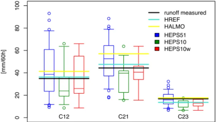
Figure 6 shows the event discharges for the two example catchments in Fig. 4 (C12, C21) and catchment C23, which captures the out-flow from all catchments and thus represents the entire study area. Results from hindcasts starting on 20 August, corresponding to 96 h lead time, are shown. The ensemble spreads for HEPS51 nicely capture both observed runoff and HREF in all three catchments. The weighted ensemble HEPS10w improves the results with respect to HEPS10 for catchment C12, while for C21 the effect of the weighting is less pronounced. In addition, HALMO shows remarkably good performance for C12 and C23 for the pre-sented lead time (96 h), as noted in the previous section. For catchment C23, all simulations show a distinct reduction in ensemble spread and error. This indicates an overall decrease in uncertainty for forecasts over larger areas (i.e. differences in forecasts for small catchments even out over larger areas). The general performance of an ensemble is determined by the relation between the error of the median of the ensem-ble with respect to the reference, and the spread of the en-semble. Assuming a perfectly calibrated probabilistic fore-cast, the following relation between the two variables should be found: the median of the error distribution should ex-actly match half the ensemble IQR (Lalaurette et al., 2005). Thus, a higher median error should be accompanied by a wider spread in order to account for the ensemble
uncer-0 2 0 4 0 6 0 8 0 1 0 0 [mm/ 6 0 h ] C12 C21 C23 runoff measured HREF HALMO HEPS51 HEPS10 HEPS10w
Fig. 6. Event discharges (mm/60h) for observed runoff (black),
HREF (turquoise), HALMO (yellow), and whisker plots for the en-semble forecasts HEPS51 (blue), HEPS10 (green) and HEPS10w (red). Results are presented for the two catchments previously shown in Fig. 4 (C12, C21) and the catchment C23, representing the whole study area. All displayed forecasts are started on 20 Au-gust.
tainty. Considering this relationship for all catchments and lead times, HEPS10 tends to slightly underestimate spread, although the weighting improves this to some degree. Both the underestimation in spread (HEPS10) as well as the im-provement through weighting (HEPS10w) can be seen for all catchments in Fig. 6. While the median of HEPS10 and HEPS10w only slightly differ, the spread of HEPS10w is providing a better coverage of the measured runoff and HREF. Strong deviations from this generalization are found for the longest lead time, where high values occurred for median errors without the necessary compensation through a widened spread (reasons for this are discussed in greater detail in Sect. 3.5). HEPS51 does not show this behavior and generally provides the necessary spread to cover the uncer-tainty.
3.4 Probabilistic verification of time series
The evaluation of exceedance probabilities and event dis-charges alone do not address the temporal evolution of the hydrographs. As a result, it is not clear whether the simu-lations peak too early or too late. Although an evaluation based on hourly time steps is quite a challenge for a model system (especially in the case of an extreme event), the next logical step is an evaluation of the temporal evolution using the Brier Skill Score (BSS). In Table 2 we compare HEPS51, the weighted ensemble HEPS10w, the unweighted HEPS10 and HALMO against HREF, using the mean event runoff from HREF as a threshold. The use of HREF as the refer-ence for the BSS calculation, in place of the observed hy-drographs, allows hydrological uncertainties to be excluded. Using HREF in place of the runoff observations generally yields higher scores (e.g., +0.11 on the median score of
Table 2. BSS for simulated runoff (relative to simulation HREF)
and related area-mean precipitation (relative to observations) during the event period for three different lead times. Middle and right columns show median scores (for the 23 catchments considered), for the different lead times and the combined median (c. median) for all catchments and lead times, respectively.
median c. median
lead time runoff precip. runoff precip.
HALMO 120/114 na na na na 96/90 0.27 0.00 72/66 0.07 0.07 HEPS10 120/114 −0.23 −0.53 0.21 0.05 96/90 0.31 0.09 72/66 0.57 0.39 HEPS10w 120/114 −0.23 −0.66 0.29 −.01 96/90 0.37 −0.01 72/66 0.59 0.37 HEPS51 120/114 0.07 −0.09 0.32 0.17 96/90 0.37 0.21 72/66 0.61 0.41
HEPS51). The skill of the precipitation forecasts (time se-ries of the catchment mean) was calculated analogously, us-ing the hourly time series of the observed spatially interpo-lated precipitation on the respective catchment as reference, and its median as threshold.
In the case of the deterministic forecast (HALMO), the longest lead time is suppressed (na) in Table 2. While show-ing good results for threshold exceedance, HALMO gener-ally has lower skill scores than the ensembles. For the lead time of 96 h, HALMO median runoff skill scores almost reach the level of HEPS10, reflecting the correct distribu-tion of precipitadistribu-tion with only a slight overestimadistribu-tion (Me-teoSchweiz, 2006). This is not visible in the median BSS for precipitation alone, as the precipitation forecast still needs to be elongated by 18 h. For the shortest lead time, the median performance of HALMO is compromised by the pronounced overestimation in precipitation and runoff.
Regarding the ensembles, an increase in skill with shorter lead times for all ensemble sizes is evident. Scores for cipitation alone suffer much more from the decrease in pre-dictability with longer lead times and are generally lower than those for runoff. This is the case, since the scores for runoff profit from the information stored within the hydro-logical system (soil moisture, status of water storages) as well as from the filtering effect of the direct input (smooth-ing through the retard(smooth-ing effect of the hydrological system through the different water storages). This applies to most of the individual catchments as well as for the mean values of the ensemble simulations.
! "! #! $! %! &! ! "'! ! !'& !'! !'& "'! ()*+,-.+*/0+ 12/+2345/..34672+ 89:;< 8(=4"! 8(=4"!> 8(=4&" ensemble size
Fig. 7. Median BSS for sampled ensembles from HEPS51 with
gradually reduced ensemble sizes, shown for catchment C10 (blue, with 90% quantile). BSS for HEPS10w (red, marked at effective ensemble size), HEPS10 (green) and HALMO (black) are addition-ally marked.
3.5 Representativeness of the reduced ensemble
In Table 2, a general loss of information due to the reduction of the ensemble size is found for runoff as well as for pre-cipitation in almost all catchments (i.e. the score is worse for HEPS10 compared to HEPS51 for the corresponding initial-ization time). The weighting of the reduced ensemble com-pensates for this loss of information to some extent. This is not the case for precipitation alone, where weighting actu-ally worsens BSS. Since the general performance of an en-semble is determined by the relation between the error of the median of the ensemble with respect to the reference and the spread of the ensemble, a higher median error should be accompanied by a wider spread to account for the uncer-tainty. Because the relation between the median error and the IQR changes through the application of the hydrological sys-tem (the median error experiences a stronger reduction than IQR), the weighting shows a different effect for precipitation. Relative shifts of the median error show a larger effect espe-cially for low scores, without being able to compensate with a widened spread.
The observed loss of information by the reduction in en-semble size (from HEPS51 to HEPS10) shown in Table 2, leads to the question of representativeness of the reduced ensemble. To test the representativeness of reduced ensem-bles and the influence of the weighting, a statistical analysis was carried out. For this purpose we decreased the member size of the full ensemble step-wise by one ensemble member from 51 to one, and sampled 1000 of the possible member
combinations of the full ensemble for each step, with the ex-ception of ensemble sizes 1, 50 and 51, where the maximum of possible member combinations was used. With a sample size of 1000, the possible member combinations are well rep-resented, while the amount of data is still easily manageable. Consideration of small ensembles leads to a negative bias of the BSS (M¨uller et al., 2005; Weigel et al., 2007a). By comparing the skill scores at the respective ensemble sizes, we do not need to correct this bias. A reduced ensemble therefore represents the full ensemble if its skill is equal to the median skill of the sampled member combinations at the respective ensemble size. The analysis was performed for all of the catchments using the evaluation time window for the three different forecast lead times.
Figure 7 shows the dependence of skill score on ensemble size for catchment C10 for the shortest lead time (72 h). The blue circles and the vertical bars mark the median BSS of the 1000 ensemble samples at each member size with 90% confi-dence interval. Some general ensemble properties are nicely reproduced: The reduction in median skill with smaller en-semble size is accompanied by an increase in spread (of the skill values). A saturation effect is also visible at member sizes of 5 to 15. For larger ensemble sizes, the median BSS no longer increases significantly, while the spread of the skill score decreases continuously. The risk of a forecast failure through an unfavorable selection of representative members is thus reduced. The choice of the ensemble size for the re-duced ensemble (10 members) seems reasonable, as it lies within the region of saturation and has a noticeable reduction in skill score spread. The BSS of HEPS10 is slightly below the median sampled BSS. Weighting the reduced ensemble (HEPS10w) further improves the match. The weighted en-semble HEPS10w is marked at the position of its effective ensemble size meff = 1 P10 n=1w2n . (5)
This reduction by a nonuniform weight (w) distribution is qualitatively understandable, when looking at the two ex-treme weighting possibilities. If all ensemble members are equally weighted (w=0.1), the unweighted case of HEPS10 is reproduced. At the other extreme, if all weight is assigned to a single ensemble member and the others receive zero weight, the effective ensemble collapses to a single mem-ber ensemble. For all other weight distributions the effective ensemble size lies somewhere in between these two extremes (Weigel et al., 2007b).
The skill score for HALMO in Fig. 7 is well below the en-semble scores, which is generally reflected in Table 2. Com-pared to the ensemble sample at member size 1 (consisting of the 51 individual ensemble members), HALMO outper-forms the ensemble median. HALMO probably profits from the smaller grid-spacing of 7 km instead of 10 km used for the ensembles. 0 10 20 30 40 50 −3.0 −2.0 −1.0 0.0 1.0 ensemble size
Brier Skill Score
HEPS10 HEPS10w HEPS51
Fig. 8. Combined BSS for 23 subcatchments and three lead times as
a function of ensemble size. The plot shows the median (bold blue line), the IQR (thin blue lines), the 90% quantile (dashed blue line) and the full range (light blue). The overlayed whisker plots show the BSS for HEPS10 (green) and HEPS10w (red).
Figure 8 combines the results shown in Fig. 7 for all catch-ments and lead times. In order for HEPS10 (or HEPS10w) to optimally represent HEPS51, the median and quantiles of the respective reduced ensemble BSS should match those of the sampled BSS at the respective ensemble size. The dian BSS of HEPS10 is slightly lower than that of the me-dian sampled BSS, and its lower quantiles show a further decrease. The weighting with the represented cluster sizes (HEPS10w) improves the match of the statistical properties, specifically for the quartiles and the median. This is an effect of the widened ensemble IQR which occurs through weight-ing (especially for the 96 h lead time as apparent from Ta-ble 2), resulting in a better representation of the ensemTa-ble uncertainty. The effect of the weighting on the ensemble me-dian error is less important in comparison to spread. This is not true for low skill values, where a weighting actually worsens the BSS. The low skill values can be matched to the longest lead time of 120 h, as apparent in Table 2, where the median skill does not benefit from weighting. Even though the weighting still increases the ensemble IQR (for 17 out of 23 forecasts), it actually decreases the spread of the 10– 90% ensemble quantile (in 18 out of 23 forecasts). The high value of the ensemble median error averaged over all catch-ments for 120 h lead time (0.17 mm, compared to 0.07 mm and 0.06 mm for 96 h and 72 h) without the necessary in-crease in spread explains the reduction of the BSS at low skills by weighting.
Figure 8 shows that not only HEPS10w, but also HEPS10 does not properly represent HEPS51 on low skills (matching
the 120 h lead time). This can be traced back to the used clustering methodology with recombination (based on twice 51 EPS members, cf. Sect. 2.2). The recombination with old forecast information favors the selection of representa-tive members with low runoff values and therefore underes-timates the event.
Besides the recombination, the clustering methodology it-self can affect the skill of the forecasts, as it is based on large-scale weather patterns over the full COSMO-LEPS domain. This does not necessarily result in the ideal set of represen-tative members for the considered, relatively small, subdo-mains (i.e. catchments), especially as the quantitative precip-itation amounts, which are of major importance for the hy-drological forecast, are not directly considered for the clus-tering (Molteni et al., 2001). As the (median) loss in skill is not dramatic, it seems justified to use the reduced ensembles, although one is faced with potentially lower skill for specific catchments and lead times.
4 Conclusions
Using the extreme Alpine flood of August 2005 as a case study, we find a good hindcast performance of the applied coupled meteorological-hydrological ensemble forecast sys-tem. Statistical tests demonstrates that the use of the re-duced ensembles with representative members seems justi-fied, while weighting further improves the skill of the system (except on low scores). The median BSS of HEPS10w of 0.29 for all catchments and lead times shows that the fore-cast system has useful skill. While the deterministic hindfore-cast shows good results for a lead time of 96 h, the forecast with a lead time of 72 h strongly overpredicts the event. This il-lustrates the effect of “badly” chosen (versus “well” chosen) initial conditions of the meteorological model, a difficulty which can be accounted for by the use of ensembles. The ad-ditional probabilistic information resulting from the ensem-ble therefore helps to classify the deterministic forecast, and provides useful information about its uncertainty.
An obvious practical application of the medium forecast ranges are “wake up calls”. The significantly higher skill of the coupled meteorological-hydrological system in compar-ison to the meteorological precipitation forecast shows the importance of the filtering through the hydrological system and the overall added benefit of the coupled model system.
To assess the applicability of the proposed meteorologic-hydrologic forecast system for day-to-day application, a hindcast study providing two years of continuous probabilis-tic hindcasts is currently in progress. While the current study, using a unique extreme event, puts the emphasis on the im-pact of the ensemble size, the work on the longer time series will concentrate on the role of the lead time, the extension to several skill scores as proposed by Laio and Tamea (2007) and an evaluation for a wide range of weather situations.
Acknowledgements. We would like to thank the Swiss Federal Office for the Environment (FOEN), the Landeswasserbauamt Voralberg and the German Weather Service (DWD) for provision of meteorological and hydrological data. Financial support is acknowledged to the Swiss National Centre for Competence in Research (NCCR-Climate) and the State Secretariat for Education and Research SER (COST 731). The aLMo weather forecasts were done at the Swiss National Supercomputing Centre (CSCS) in Manno, Switzerland. For the provision of Fig. 1 we express our thanks to C. Frei from MeteoSwiss. Finally, we would like to acknowledge J. Gurtz and M. Zappa for support with hydrological questions.
Edited by: A. M. Rossa
Reviewed by: K. Schr¨oter and another anonymous referee
References
Ahrens, B.: Evaluation of precipitation forecasting with the limited area model ALADIN in an alpine watershed, Meteorol. Z., 12, 245–255, doi:10.1127/0941-2948/2003/0012-0245, 2003. Ahrens, B. and Walser, A.: Information-based skill scores for
probabilistic forecasts, Mon. Weather Rev., 136, 352–363, doi: 10.1175/2007MWR1931.1, 2008.
Bergstr¨om, S. and Forsman, A.: Development of a conceptual deter-ministic rainfall-runoff model., Nord. Hydrol., 4, 147–170, 1973. Bezzola, G. R. and Hegg, C. (Eds.): Ereignisanalyse Hochwasser 2005, Teil 1 – Prozesse, Sch¨aden und erste Einordnung, no. 0707 in Umweltwissen, Bundesamt f¨ur Umwelt BAFU, Bern; Eidg. Forschungsanstalt WSL, Birmensdorf, http://www.bafu.admin. ch/php/modules/shop/files/pdf/php8BthWS.pdf, 2007.
Buizza, R.: Encyclopaedia of Atmospheric Sciences, chap. Weather Prediction: Ensemble Prediction, pp. 2546–2557, Academic Press, London, 2003.
Buizza, R. and Palmer, T.: The singular-vector structure of the at-mospheric global circulation, J. Atmos. Sci., 52, 1434–1456, doi: 10.1175/1520-0469(1995)052h1434:TSVSOTi2.0.CO;2, 1995. Collier, C. G.: Flash flood forecasting: What are the limits of
pre-dictability?, Q. J. Roy. Meteorol. Soc., 133, 3–23, doi:10.1002/ qj.29, 2007.
Fl¨ugel, W.-A.: Combining GIS with regional hydrological mod-elling using hydrological response units (HRUs): An applica-tion from Germany, Math. Comput. Simulat., 43, 297–304, doi: doi:10.1016/S0378-4754(97)00013-X, 1997.
Gurtz, J., Baltensweiler, A., and Lang, H.: Spatially dis-tributed hydrotope-based modelling of evapotranspiration and runoff in mountainous basins, Hydrol. Process., 13, 2751– 2768, doi:10.1002/(SICI)1099-1085(19991215)13:17h2751:: AID-HYP897i3.0.CO;2-O, 1999.
Gurtz, J., Zappa, M., Jasper, K., Lang, H., Verbunt, M., Badoux, A., and Vitvar, T.: A comparative study in modelling runoff and its components in two mountainous catchments, Hydrol. Process., 17, 297–311, doi:10.1002/hyp.1125, 2003.
Hohenegger, C., Walser, A., and Sch¨ar, C.: Cloud-resolving en-semble simulations of the August 2005 Alpine flood, Q. J. Roy. Meteorol. Soc., accepted, 2008.
Houtekamer, P. L., Lefaivre, L., Derome, J., Ritchie, H., and Mitchell, H. L.: A system simulation approach to ensemble
prediction, Mon. Weather Rev., 124, 1225–1242, doi:10.1175/ 1520-0493(1996)124h1225:ASSATEi2.0.CO;2, 1996.
Komma, J., Reszler, C., Bl¨oschl, G., and Haiden, T.: Ensemble prediction of floods – catchment non-linearity and forecast prob-abilities, Nat. Hazards Earth Syst. Sci., 7, 431–444, 2007, http://www.nat-hazards-earth-syst-sci.net/7/431/2007/.
Laio, F. and Tamea, S.: Verification tools for probabilistic forecasts of continuous hydrological variables, Hydrol. Earth Syst. Sci., 11, 1267–1277, 2007,
http://www.hydrol-earth-syst-sci.net/11/1267/2007/.
Lalaurette, F., Bidlot, J., Ferranti, L., Ghelli, A., Grazzini, F., Leutbecher, M., Paulsen, J.-E., and Viterbo, P.: Verification statistics and evaluations of ECMWF forecasts in 2003–2004, Tech. Rep. 463, ECMWF, Shinfield Park Reading, Berks RG2 9AX, http://www.ecmwf.int/publications/library/ecpublications/
pdf/tm/401-500/tm463.pdf, 2005.
Legates, D. R. and McCabe, G. J.: Evaluating the use of “goodness-of-fit” measures in hydrologic and hydroclimatic model validation, Water Resour. Res., 35, 233–242, doi:10.1029/ 1998WR900018, 1999.
Lindstr¨om, G., Johansson, B., Persson, M., Gardelin, M., and Bergstr¨om, S.: Development and test of the distributed HBV-96 hydrological model, J. Hydrol., 201, 272–288, doi:10.1016/ S0022-1694(97)00041-3, 1997.
Marsigli, C., Boccanera, F., Montani, A., and Paccagnella, T.: The COSMO-LEPS mesoscale ensemble system: Validation of the methodology and verification, Nonlin. Processes Geophys., 12, 527–536, 2005,
http://www.nonlin-processes-geophys.net/12/527/2005/. MeteoSchweiz: Starkniederschlagsereignis August 2005,
Ar-beitsbericht 211, MeteoSchweiz, http://www.meteoschweiz. admin.ch/web/de/forschung/publikationen/alle publikationen/ starkniederschlagsereignis.html, 2006.
Molteni, F., Buizza, R., Palmer, T., and Petroliagis, T.: The ECMWF Ensemble Prediction System: Methodology and vali-dation, Q. J. Roy. Meteorol. Soc., 122, 73–119, doi:10.1002/qj. 49712252905, 1996.
Molteni, F., Buizza, R., Marsigli, C., Montani, A., Nerozzi, F., and Paccagnelli, T.: A Strategy for high-resolution ensemble predic-tion. I: Definition of representative members and global-model experiments., Q. J. Roy. Meteorol. Soc., 127, 2069–2094, doi: 10.1256/smsqj.57611, 2001.
Montani, A., Capaldo, M., Cesari, D., Marsigli, C., Modigliani, U., Nerozzi, F., Paccagnella, T., Patruno, P., and Tibaldi, S.: Operational limited-area ensemble forecasts based on the Lokal Modell, ECMWF Newsletter, 98, 2–7, http://www.ecmwf.int/ publications/newsletters/pdf/98.pdf, 2003.
M¨uller, W. A., Appenzeller, C., Doblas-Reyes, F. J., and Liniger, M. A.: A debiased ranked probability skill score to evaluate prob-abilistic ensemble forecasts with small ensemble sizes, J. Cli-mate, 18, 1513–1523, doi:10.1175/JCLI3361.1, 2005.
Nash, J. E. and Sutcliffe, J. V.: River flow forecasting through con-ceptual models: Part 1 – A discussion of principles, J. Hydrol., 10, 282–290, doi:10.1016/0022-1694(70)90255-6, 1970. Nurmi, P.: Recommendations on the verification of local weather
forecasts, Tech. Rep. 430, ECMWF, Shinfield Park Reading, Berks RG2 9AX, http://www.ecmwf.int/publications/library/ ecpublications/ pdf/tm/401-500/tm430.pdf, 2003.
Pappenberger, F. and Beven, K. J.: Ignorance is bliss: Or seven
reasons not to use uncertainty analysis, Water Resour. Res., 42, 1–8, doi:10.1029/2005WR004820, 2006.
Pappenberger, F., Beven, K., Hunter, N., Bates, P., Gouweleeuw, B., Thielen, J., and de Roo, A.: Cascading model uncertainty from medium range weather forecasts (10 days) trough a rainfall-runoff model to flood inundation predictions within the European Flood Forecasting System (EFFS), Hydrol. Earth Syst. Sci., 9, 381–393, 2005,
http://www.hydrol-earth-syst-sci.net/9/381/2005/.
Roulin, E. and Vannitsem, S.: Skill of Medium-Range Hydrological Ensemble Predictions, J. Hydrometeorol., 6, 729–744, doi:10. 1175/JHM436.1, 2005.
Rousset, F., Habets, F., Martin, E., and Noilhan, J.: Ensemble streamflow forecasts over France, ECMWF Newsletter, 111, 21– 27, http://www.ecmwf.int/publications/newsletters/pdf/111.pdf, 2007.
Siccardi, F., Boni, G., Ferraris, L., and Rudari, R.: A hydromete-orological approach for probabilistic flood forecast, J. Geophys. Res., 110, 1–9, doi:10.1029/2004JD005314, 2005.
Steppeler, J., Doms, G., Sch¨attler, U., Bitzer, H.-W., Gassmann, A., Damrath, U., and Gregoric, G.: Meso-gamma scale forecasts using the nonhydrostatic model LM, Meteorol. Atmos. Phys., 82, 75–96, doi:10.1007/s00703-001-0592-9, 2003.
Todini, E.: Role and treatment of uncertainty in real-time flood forecasting, Hydrol. Process., 18, 2743–2746, doi:10.1002/hyp. 5687, 2004.
Toth, Z. and Kalnay, E.: Ensemble forecasting at NCEP and the breeding method, Mon. Weather Rev., 125, 3297–3319, doi:10. 1175/1520-0493(1997)125h3297:EFANATi2.0.CO;2, 1997. Verbunt, M., Zappa, M., Gurtz, J., and Kaufmann, P.: Verification
of a coupled hydrometeorological modelling approach for alpine tributaries in the Rhine basin, J. Hydrol., 324, 224–238, doi:10. 1016/j.jhydrol.2005.09.036, 2006.
Verbunt, M., Walser, A., Gurtz, J., Montani, A., and Sch¨ar, C.: Probabilistic Flood Forecasting with a Limited-Area Ensemble Prediction System: Selected Case Studies, J. Hydrometeorol., 8, 897–909, doi:10.1175/JHM594.1, 2007.
Viviroli, D., Gurtz, J., and Zappa, M.: The Hydrological Modelling System PREVAH, Geographica Bernensia P40, Institute of Ge-ography, University of Berne, 2007.
Vrugt, J. A., Diks, C. G. H., Gupta, H. V., Bouten, W., and Verstraten, J. M.: Improved treatment of uncertainty in hydro-logic modeling: Combining the strengths of global optimiza-tion and data assimilaoptimiza-tion, Water Resour. Res., 41, 1–17, doi: 10.1029/2004WR003059, 2005.
Weigel, A. P., Liniger, M. A., and Appenzeller, C.: The Discrete Brier and Ranked Probability Skill Scores, Mon. Weather Rev., 135, 118–124, doi:10.1175/MWR3280.1, 2007a.
Weigel, A. P., Liniger, M. A., and Appenzeller, C.: Generaliza-tion of the Discrete Brier and Ranked Probability Skill Scores for Weighted Multi-model Ensemble Forecasts, Mon. Weather Rev., 135, 2778– 2785, doi:10.1175/MWR3428.1, 2007b. Wilks, D.: Statistical methods in the atmospheric sciences, vol. 91
of International geophysics series, Elsevier, Amsterdam, 2nd edn., 2006.
Zappa, M.: Multiple-Response Verification of a Distributed Hy-drological Model at Different Spatial Scales, Ph.D. thesis, ETH Zurich, diss. ETH No. 14895, 2002.