Reconstructing depth-averaged open-channel flows using image velocimetry and photogrammetry

HAL Id: hal-01855840

https://hal-edf.archives-ouvertes.fr/hal-01855840

Submitted on 20 Feb 2019

HAL is a multi-disciplinary open access

archive for the deposit and dissemination of

sci-entific research documents, whether they are

pub-lished or not. The documents may come from

teaching and research institutions in France or

abroad, or from public or private research centers.

L’archive ouverte pluridisciplinaire HAL, est

destinée au dépôt et à la diffusion de documents

scientifiques de niveau recherche, publiés ou non,

émanant des établissements d’enseignement et de

recherche français ou étrangers, des laboratoires

publics ou privés.

Reconstructing depth-averaged open-channel flows using

image velocimetry and photogrammetry

Guillaume Piton, Alain Recking, Jerome Le Coz, Hervé Bellot, Alexandre

Hauet, Magali Jodeau

To cite this version:

Guillaume Piton, Alain Recking, Jerome Le Coz, Hervé Bellot, Alexandre Hauet, et al.. Reconstructing

depth-averaged open-channel flows using image velocimetry and photogrammetry. Water Resources

Research, American Geophysical Union, 2018, 54 (6), pp.4164-4179. �10.1029/2017WR021314�.

�hal-01855840�

Piton

et

al.

(2018)

W

ater

R

esour

ces

R

ese

ar

ch

,

54.

DOI:10.1029/2017WR021314

,

first

author’s

p

ersonal

cop

y

Reconstructing depth-averaged open-channel flows using image

velocimetry and photogrammetry

Guillaume PITON

, Alain RECKING

_{, J´}

_erˆ

_{ome LE COZ}

_{, Herv´}

_{e BELLOT}

_{, Alexandre}

HAUET

_{, and Magali JODEAU}

1

_{Univ. Grenoble Alpes, Irstea, UR ETGR, Grenoble, France.}

_{Irstea, UR HHLY, Hydrology-Hydraulics, Villeurbanne, France.}

3

_Electricit´

_{e de France, DTG, Grenoble, France.}

_Electricit´

_{e de France, LNHE, Chatou, France.}

February 20, 2019

This is the personal first author’s version of a paper published in Water Resource Research on 2018. To cite the paper:

Piton, G., Recking, A., Le Coz, J., Bellot,H., Hauet, A., & Jodeau, M. (2018). Reconstructing depth-averaged

openchannel flows using image velocimetry and photogrammetry. Water Resources Research, 54. DOI:10.1029/2017WR021314

• Bedload-laden flows on steep slopes are complex and poorly known processes with highly mobile boundaries • The paper proposes a complete procedure to reconstruct depth-averaged flow spatial distribution

• The method combines Large Scale-PIV and Structure-from-Motion photogrammetry in a friction law

Abstract

Steep streams with massive sediment supply are among the most complex systems to study, even in the laboratory. Their shallow sediment-laden flows create self-adjusting bed geometries that evolve rapidly. Often, morphological changes and flow processes cannot be dissociated. Because these very shallow and unstable flows cannot be equipped with measurement sensors, image analysis techniques, such as photogrammetry (e.g., structure-from-motion, SfM) and large-scale particle image velocimetry (LSPIV), are interesting options for capturing the characteristics of these systems. The present work describes a complete procedure using both techniques to measure spatially distributed surface velocity and bed properties (deposit patterns, channel slope, local roughness). The velocity data are used to assess the local flow directions along which the channel slope and roughness are extracted from the SfM digital elevation models. Ferguson’s ”variable power equation” friction law, having been previously validated by comparison with approximately 100 local flow depth measurements, was used in a second step with the collected data to reconstruct a complete mapping of the depth-averaged flows, thereby enabling a comprehensive analysis of the hydro-geomorphic system where shallow water equations apply. The assumptions, details, use of the friction law with roughness standard deviation rather than diameter as parameter and limitations of the procedure as well as possible sources of errors are discussed here, along with possibilities for improvements. This affordable and simple-to-implement procedure can provide a large amount of data, allowing for a more comprehensive analysis of complex hydraulic systems.

Piton

et

al.

(2018)

W

ater

R

esour

ces

R

ese

ar

ch

,

54.

DOI:10.1029/2017WR021314

,

first

author’s

p

ersonal

cop

y

1

Introduction

Hydraulic numerical models basically resolve equations that were initially developed and validated with field and laboratory measurements. Measuring water velocity and depth remains thus a keystone of studies on insufficiently known river systems. These key parameters are, however, sometimes complicated to estimate; especially in cases of marked sediment transport and fast geomorphic changes as experienced, for instance, in steep streams (i.e., with bed slope > 0.02). Small-scale modeling in laboratory is particularly useful in this case because the physics of sediment transport and steep slope hydraulics is not yet sufficiently understood, limiting the capacity of numerical models. While several attempts have been made to analytically address these processes, there are no data for their validation (Ferguson 2007; Recking et al. 2016; Piton and Recking 2017).

Most hydraulic studies of steep slope streams have been carried out in laterally constrained conditions, i.e., with a flow width limited by the flume side walls. Lateral constraints facilitate lateral observations and detailed flow profile measurements (e.g., Revil-Baudard et al. 2015), as well as studies of longitudinal profile adjustments (e.g., Recking et al. 2009), although they neglect the capacity of the river to adjust its width to the flows. The lateral constraint usually figuring solid banks is necessary in numerous studies of in-channel processes, e.g., in step-pool channels whose stability is controlled by channel width and bank roughness (Zimmermann and Church 2001).

On the contrary, the lateral constraint relaxation may play a key role in the emergence of geomorphic processes such as braiding, avulsion, and fan creation, possibly resulting in changes in the equilibrium slopes (Piton and Recking 2016a), thus fundamentally different than the laterally constrained conditions. Such laterally unconstrained systems are less known than laterally constrained ones because they are more complicated to study (e.g., it is not possible to perform measurements through side walls). Braided river dynamics or alluvial fan formation are good examples of such laterally unconstrained systems for which insights into their morphodynamics exist but much less so regarding their hydraulics (Reitz and Jerolmack 2012; Leduc et al. 2015). The fan-like deposition process occurring in bedload retention basins located in mountain streams has recently been reproduced in the IRSTEA Grenoble flume. These experiments are used here as the basis for the development of the method. The aim was to characterize the hydraulics over sediment deposition in 10%-steep retention basins. It is possibly one of the most restrictive situation, with depths over coarse sediments in highly mobile, out-of-equilibrium, and rapidly evolving beds under flashy, massive bedload deposition.

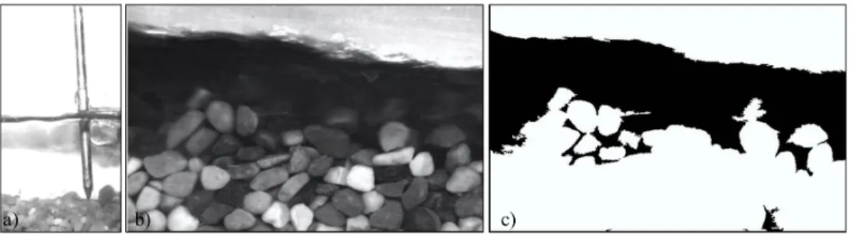
The study of steep flows in this kind of small-scale model is jeopardized by the difficulty of measuring such shallow and morphologically active systems. Water depth may be measured at specific locations using a point gauge (Fig. 1a), ultrasonics probes, or green and red coupled lasers. However, these techniques only give local information of a fundamentally very active and heterogeneous system. Numerous measurements should be taken to reduce the depth measurement random variations related to free surface and mobile bed instabilities (Fig. 1b-c).

Figure 1: Side views of steep flows over a mobile bed composed of nearly uniform grains: a) illustration of the use of a point gauge: epistemic uncertainty related to the variable bed level and free surface, b) side view showing mobile grain clusters and perturbed free surface highlighting how uncertain the water depth measurement is, c) same image after threshold analysis showing the local variability of the water depth in bedload-laden flows

Generally, all direct measurements with intrusive velocity sensors (e.g., velocity profiler, flow meters) are inap-propriate because: (i) the sensor size can be larger than the flow depth, (ii) transported sediments may damage sensors, and (iii) the sediment transport intensity makes flow paths unstable, shifting and wandering in the flume. In addition to the planimetric instability, the vertical bed adjustments reach several times the water depth, so that the sensors are intermittently buried in sediment or perched over a degrading channel. In addition to depth, it is interesting to have information on flow velocities. Velocity measurements have usually been carried out with injections of salt (Smart and Jaeggi 1983; Cao 1985; Rickenmann 1990) and dye (Recking et al. 2008a; Ghilardi

Piton

et

al.

(2018)

W

ater

R

esour

ces

R

ese

ar

ch

,

54.

DOI:10.1029/2017WR021314

,

first

author’s

p

ersonal

cop

y

Considering all the difficulties of measuring the depth average velocity, an alternative is to measure the spa-tially distributed surface flow velocity by image analysis. Particle tracking velocimetry (PTV) consists in tracking individual particles between images pairs, giving a Lagrangian description of velocity fields (Maas et al. 1993). In contrast, particle image velocimetry (PIV) is a Eulerian approach, which consists in tracking patterns advected by the flows, often seeded tracers (Willert and Gharib 1991).

In cases where intrusive measures are prohibited, the LSPIV technique (large-scale PIV, Fujita et al. 1998) enables measurements in difficult flow conditions (Jodeau et al. 2008; Muste et al. 2010; Dramais et al. 2011; Muste et al. 2014; Detert and Weitbrecht 2015), as well as in fast torrential flows (Le Coz et al. 2010; Le Boursicaud et al. 2016; Stumpf et al. 2016). LSPIV has proved to be accurate also in the laboratory on low submersion and relatively steep slopes (Nord et al. 2009; Legout et al. 2012).

Detailed photogrammetric measurements are complementary to the LSPIV technique. The structure-from-motion (SFM) technique is also a simple and affordable image analysis technique that is increasingly used in geoscience (Westoby et al. 2012; Brasington et al. 2012; Stumpf et al. 2016; V´azquez-Tarr´ıo et al. 2017). These two affordable image analysis measurement techniques, already used in the field for river discharge measurement (Stumpf et al. 2016; Detert et al. 2017), were combined here in a novel way to reconstruct flow depths of very rapidly evolving geomorphic systems. In the present work, a friction law – i.e., an equation relating water depth to velocity, slope, and roughness – was validated with local depth measurements using a point gauge, and then used to reconstruct water depth distributions from LSPIV and SfM data.

This paper proposes a low-cost, complete methodology comprising (i) the LSPIV measurement of surface velocity, (ii) the photogrammetric measurement of the bed topography and bed roughness deduced from the digital elevation models (DEM) of the bed, and (iii) the use of a friction law to determine flow depths from the measured slopes, roughnesses, and flow velocities. Possible improvements of the technique are finally discussed. All experimental details are provided in Piton (2016, p. 131), and therefore only a summary is given here.

2

Experimental and measurement set-up

2.1

Flume, sediment mixtures, and feeding

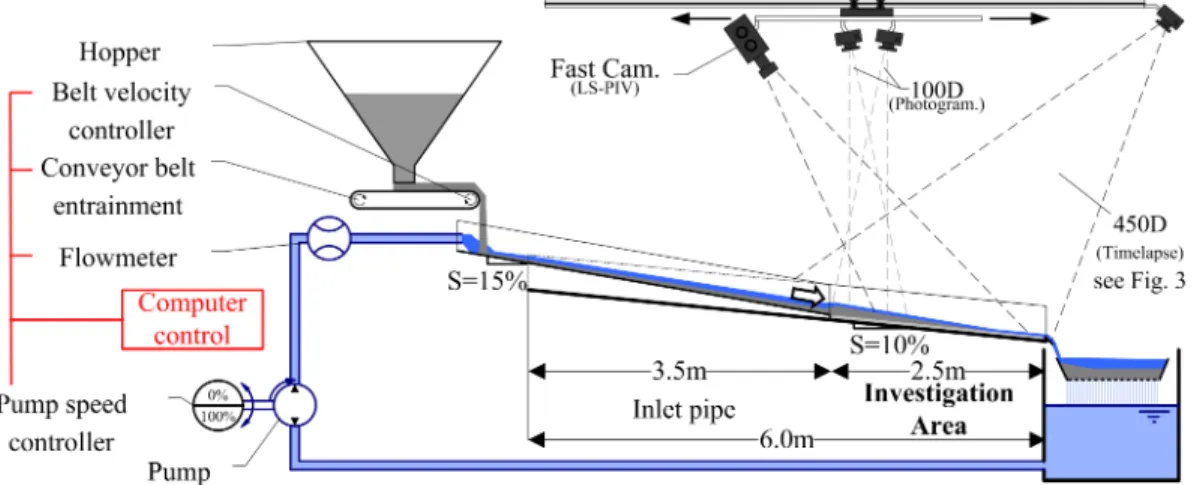
The flume was 6 m long, 1.25 m wide, and 0.4 m deep (Fig. 2). Its varying slope was fixed at 10% (5.7◦) for all runs. All flow measurements were done within the ”investigation area,” i.e., in the 2.5-m-long downstream part of the flume (Fig. 3). The investigation area was manually levelled before each experiment, leaving behind a transversally flat bed with a sediment thickness of ≈ 5 cm that represented a dredged bedload retention basin. If this layer was eroded to the flume bottom in any point, the run was stopped.

Figure 2: Experiment set-up : sediment-fed configuration and recirculation of water with four cameras for image acquisition

Hydrographs were used with a maximum discharge varying in the range 1.62-2.75 l/s. Water discharge was remotely controlled by varying the pump velocity, and measured with a flowmeter (Krohne IPC 080) at a

10-Piton

et

al.

(2018)

W

ater

R

esour

ces

R

ese

ar

ch

,

54.

DOI:10.1029/2017WR021314

,

first

author’s

p

ersonal

cop

y

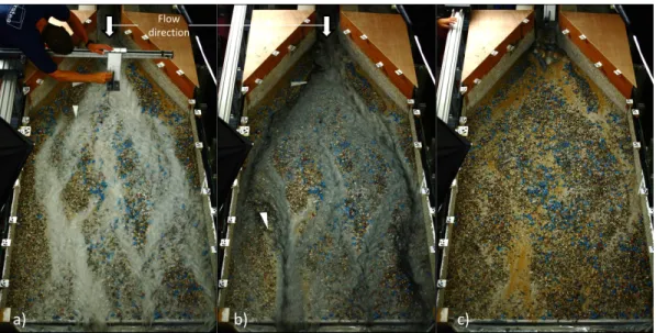
Figure 3: Images of the investigation area: a) flow depth local measurement with a point gauge, a few seconds later, b) flow seeded with charcoal powder clouds during the LSPIV image capture, immediately followed by c) stopping of the experiment and drained-bed image capture for SfM photogrammetry acquisition. Only measures with negligible morphological changes between LSPIV and SfM acquisitions were used in flow reconstruction. The white triangle marks the gauge measure abscissa. Note that the flow may touch one side wall but remains an unconfined flow because the other bank can erode or aggrade to adjust the channel width.

Table 1: Experimental plan

GSD D50 D84 Q Qs Tpeak C=Qs/Q Nrun NDEM NP IV Nwater

code [mm] [mm] [l/s] [g/s] [min] [%] depth

1 3.8 8.1 2.75 73-292 22.5-90 1-4 4 22 14 28

2 2.4 6.2 1.62-2.75 146-213 30-45 2-5 9 68 47 68

Note: DX diameter such that X is finer, Q: peak water discharge range, Qs: peak solid discharge range, Tpeak: duration before hydrograph peak, C: sediment concentration assuming a sediment density of 2.65, Nrun: total number hydrograph tested; NDEM: total number of digital elevation models (DEM) acquisition; NP IV: total number of LSPIV acquisition; and Nwaterdepth: total number of reference points, i.e., point gauge water depth measurements

Hz frequency (accuracy ±0.03 l/s). Typical values of boundary conditions and the total numbers of runs and measurements are given in Table 1. Figure 4 exemplifies one run where four DEM acquisitions were performed: initial and final states and two flowing conditions where one SfM acquisition was coupled with one LSPIV acquisition. The flow reconstruction method presented in the paper is later applied to these SfM-LSPIV coupled dataset. As a consequence, two flow configuration were for instance reconstructed from the run exemplified in Figure 4.

The sediment feeder was composed of a hopper over a conveyor belt. The conveyor belt delivered sediment in a pipe that was more than 3.5 m long and 15% steep, where water and sediment mixed. It had coarse grains glued on the bottom (15–20 mm in diameter), preventing the flow from accelerating excessively. A few large boulders (diameter 30—50 mm) were additionally placed at the pipe outlet, i.e., at the basin inlet to dissipate the flow energy and prevent the possible formation of a scouring jet flow (Fig. 3c). Once the basin began to fill with deposit, the boulders were buried and the pipe was progressively back-filled, decreasing the flow slope and its energy. The 15% steepness of the pipe slope was chosen so as to minimize the back-filling length that would induce sediment buffering (Piton and Recking 2016b).

Two sediment mixtures were used, hereafter referred to as GSD1 and GSD2, consisting of natural, poorly sorted sediment with diameters from 0.2 to 20 mm (Table 1). The two mixtures have a ratio of fine / medium / large grains similar to natural grain size distributions observed in streams at 9%– − 14% steep, sorting ratiopD84/D16

Piton

et

al.

(2018)

W

ater

R

esour

ces

R

ese

ar

ch

,

54.

DOI:10.1029/2017WR021314

,

first

author’s

p

ersonal

cop

y

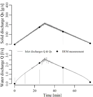
Figure 4: Typical boundary conditions: solid and water discharges at the inlet; black diamonds indicate time of LSPIV and SfM measurements; here the experiment was stopped twice, the data acquired are analyzed in subsequent figures (GSD2, peak water discharge: 2.7 l/s, peak solid discharge: 214 g/s, time to peak: 30 min).

2.2

Water depth measurement

A movable point gauge was used to measure the flow surface and bed elevations usually in one point in the center of the flow (e.g., Fig. 3a). As discussed in the introduction, this local measurement was simply used to select the suitable friction law that was extended to the whole flume in a second step. The gauge accuracy on solid, stable elements is as low as 0.01 mm. However, the highly disturbed free surface typical of steep flows on rough beds (e.g., Fig. 1b), and the dyed opaque flows with moving sediment transported on the bed (e.g., Fig. 3b), impaired the measurement accuracy. Based on our experience, the uncertainties were assumed to be ± 2 mm for the free surface level ZF S, and ± 5 mm for the bed level ZB. As a consequence, the accuracy of the water depth estimations coming from gauge measurements (d = ZF S− ZB) was ± 5.4 mm (quadratic sum used in error propagation, JCGM 2008). A total of 61 LSPIV acquisitions and 96 point gauge measurements were performed within the analyzed runs (Table 1).These point-gauge water depth measurements are hereafter referred to as ”reference points”. They were used for comparison with the water depth computed using LSPIV and SfM measurements (see below).

2.3

Image acquisition

A 6-m-long rail was fixed at the laboratory ceiling, about 2 m above the flume axis (Fig. 2). A trolley circulated on the rail, carrying a high-speed camera Phototron FASTCAM (focal length: 35 mm, 10 Mpix/frame, equipped with a polarizing filter minimizing light reflections on the free surface), and two CANON 100D cameras (focal length: 28 mm, 18 Mpix/frame). In addition, a CANON 450D camera (focal length: 32 mm, 12 Mpix/frame) was fixed at the downstream end of the rail, taking pictures every 5 seconds to later edit time-lapse videos of each experiment (e.g., Fig. 3). All the cameras were remotely controlled from a computer. Special attention was paid to ensure a homogeneous distribution of the light intensity, a key point in LSPIV (Muste et al. 2004; Kantoush et al. 2011): 4 lights directly illuminated the investigation area from its edges (2 × 250 Watts and 2 × 500 Watts, continuous current necessary if videos are acquired at frequency > 50 − 60 Hz).

2.4

LSPIV measurements

The Fudaa LSPIV software (https://forge.irstea.fr/projects/fudaa-lspiv) has been used within this work (Le Coz et al. 2014; Hauet et al. 2014).

For each measurement, the fast camera took videos of the flow at 125 frames/s for 10 seconds. Under this frequency, patterns moved strictly less than 12 pixels per image couple (spatial resolution ≈ 3.8 mm/pix). A series

Piton

et

al.

(2018)

W

ater

R

esour

ces

R

ese

ar

ch

,

54.

DOI:10.1029/2017WR021314

,

first

author’s

p

ersonal

cop

y

50 images and 20 images, respectively, were sufficient to grasp a correct value of the velocity, and that more images did not improve the results. Based on these N images, correlation analysis built N-1 velocity spatial distributions with the PIV method, i.e., by tracking the displacements of patterns in the orthorectified-image pairs (Muste et al. 2010). The correlation coefficient between image pairs, a proxy of the tracking quality, was typically of 0.8±0.1, indicating good correlations. The searching and investigation areas, typical LSPIV method parameters, were rectangles with 12*8- and 20*20-pixel sides, respectively. These sizes enable tracking of pattern in a dozen centimeter-wide channels with velocities of up to 2 m/s (a value that has never been reached). In total, 24 ground control points were used to scale the images and orthorectify them (white targets in Fig. 3).Their X, Y, Z positions were measured with a total station (accuracy ±1 mm in all directions).

Figure 5: Surface velocities: a) Interpolated mean velocity VX,Y on a regular grid (∆X = ∆Y = 5mm), and b) zoom with both interpolated velocity field and LSPIV velocity vectors higher than 0.02 m/s (GSD2, Ql=1.7 l/s, t=48 min)

Some classic experimental adjustments were necessary (see Muste et al. 2004; Kantoush et al. 2011, for recom-mendations). Using white-dyed water with T iO2 powder and flow massive seeding with crushed charcoal powder

resulted in a satisfactory estimation of the surface velocity see details in Piton 2016, p. 139.

Surface velocity measurements VLSP IV that contained ≈ 20, 000 points (on an skewed grid with a total area ≈ 1 m×2 m) were linearly interpolated on a regular grid. This grid, which supported the resulting flow field (Fig. 5), was relatively coarse (∆X = ∆Y = 5 mm, i.e., ≈ 75, 000 VX,Y interpolated points per acquisition); more detailed grids, requiring more computational time, could be built if necessary. In addition, these surface velocities were transformed into depth-averaged velocities VX,Y by multiplying VLSP IV by the velocity index α = depth-averaged velocity / surface velocity. Several studies reported that α varies weakly, even in relatively low submergence (Polatel 2006; Muste et al. 2010; Le Coz et al. 2010; Legout et al. 2012; Welber et al. 2016). It has thus been assumed that α = 0.85 ± 0.04 based on Muste et al. (2010) recommendations and Polatel (2006, p. 39) variability data. More details about this assumption are provided in the Discussion.

Piton

et

al.

(2018)

W

ater

R

esour

ces

R

ese

ar

ch

,

54.

DOI:10.1029/2017WR021314

,

first

author’s

p

ersonal

cop

y

2.5

Photogrammetry by Structure from Motion

After LSPIV image acquisition and stopping of the experiment, the flume was drained (Fig. 3b to c). High-quality pictures of the bed were taken with the trolley cameras to be used in a photogrammetry software (Agisoft Photoscan). The same ground control points as for the LSPIV were used to scale the images and orthorectify them. The classic SfM procedure was then applied (Westoby et al. 2012; Agisoft LLC 2014): (i) positioning of the ground control points in each image, (ii) back calculation of camera alignments, (iii) construction of a dense point cloud by cross-correlation between images, and (iv) construction of a 3D polygonal mesh based on the dense point cloud. In addition, (v) orthorectified high-definition images of the complete flume were reconstructed (25 pix/mm2₎

and (vi) high-density digital elevation models (DEM) were extracted from the mesh as bed elevation matrices ZX,Y (∆X = ∆Y = 1 mm, i.e., 3,125,000 elevation points per acquisition). Considering the camera resolution and coverage, it would have been possible to increase the DEM density by one order of magnitude. However, the data density of these DEMs was reasonably heavy to handle while being sufficient to describe the topography and armoring of the deposits (mean diameters of the GSD 1 and 2 were respectively 6.4 and 4.9 mm). The vertical accuracy of the measurement was estimated to ±1 mm in our experimental conditions (Le Guern 2014).

2.6

Measurement protocol

Briefly, the complete measurement procedure that was applied several times in each run, and which has been detailed in the previous sections, is as follows:

1. One or two point gauge measurements (Fig. 3a);

2. Triggering of fast camera acquisition and charcoal seeding (Fig. 3b);

3. Instantaneous stopping of the pump a few seconds before the charcoal patterns reached the flume outlet. The flume was then drained in about 5 to 10 seconds (Fig. 3b-c). These three steps usually took less than 30 seconds (back analysis from the experiment time-lapse videos);

4. Structure from motion photogrammetry of the drained deposit (≈ 30 images); 5. Instantaneous restarting of the pump, and continuing of the experimental run.

The SfM acquisition was cancelled and the LSPIV measurement data were removed if for any reason stopping the flow took too much time or if clear morphological changes occurred between the point gauge measurement and the flume draining. Morphological changes were assessed visually by looking for obvious erosion and deposit, changes in the channel direction or evidence of changing grain sorting or roughness. Attention was focused on this point at this stage of the experiment.

It could be argued that this necessary instantaneous flow stopping and restarting may disturb the sediment transport process and morphology. Local bias as less steep banks or filled scour holes may exist, like other bias typical of small-scale modelling (Heller 2011). However, the method presented in this paper aims at using the channel-scale geomorphology to reconstruct the hydraulics, not to study local phenomena. In equivalent experiments of massive bedload deposition, Ishikawa et al. (1996) and Frey et al. (1999) demonstrated that the initial deposit morphology did not influence the final one: these out-of-equilibrium, very active, depositing flows tend to rework rapidly all the morphology. Recking et al. (2009) similarly confirmed that instantaneous stopping and restarting of flow and bedload transport in narrow flume experiments did not influence the long-term morphology changes. We verified this using an experiment repeated twice: the first time stopping only twice, the second time stopping seven times. At the full experiment scale, geomorphic behaviours are similar with for instance the same envelope of deposition slopes. At equivalent time durations, the morphologies were similar in the natural range of stochastic variability. The deposit thicknesses had for instance same statistics: probability distribution functions with nearly same mean values and standard deviation of the order of magnitude of channel depths: 2-–3 cm, i.e., the channels and bars had different locations but similar vertical development.

We consequently assume that, providing that sufficient time was allowed and morphological activity was observed between the two measurements, the previous stopping/restarting did not affect the morphology permanently and thus the subsequent measurement. This lack of ”memory” of the sediment transport system (Jerolmack and Paola 2010), and the inherent complexity of poorly sorted bedload transport (Van De Wiel and Coulthard 2010) enable such stopping of the experiment, but on the other hand they make it impossible to repeat measurements of strictly the same flow and bed, due to the chaotic system behavior.

Piton

et

al.

(2018)

W

ater

R

esour

ces

R

ese

ar

ch

,

54.

DOI:10.1029/2017WR021314

,

first

author’s

p

ersonal

cop

y

3

Channel bed characterization

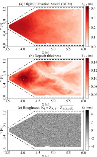
Several proxies, i.e., indirect indicators, of both the deposit thickness and the surface roughness were extracted from the DEMs and the HD orthorectified images (Fig. 6).

Figure 6: Bed topography data: a) Bed elevation ZX,Y; b) Deposit thickness TX,Y; and c) Surface roughness KsX,Y (GSD2, Ql=2.2 l/s, t=25 min)

3.1

Bed elevation data

The elevation field ZX,Y could be used to observe the bulk deposit topography (Fig. 6a). By subtraction of the flume bottom slope, the deposit thickness TX,Y is deduced (Fig. 6b) and produces a clearer view of the deposit morphology.

A local roughness indicator KsX,Y was computed by subtracting the mean local bed elevation to the point bed elevation ZX,Y, similarly to Brasington et al. (2012) or V´azquez-Tarr´ıo et al. (2017). The mean local bed elevation is averaged over a DM AX-side square, centered on the point (one value per mm2-pixel), with DM AX the coarsest grain diameter (20 mm). KsX,Y is an indicator of the point elevation compared with the local mean elevation. It tends to 0 in smooth areas (Fig. 6c), while it is positive or negative where grains protrude from the bed level. Smooth and rough areas, i.e., covered with fine sands or paved by coarse gravels can easily be distinguished on the

KsX,Y maps.

The ZX,Y and KsX,Y are matrix from which it was possible to extract the slope and roughness that are basic inputs of any friction law used to reconstruct flow fields. However, considering that the flows were not laterally constrained, their directions, along which the relevant slope and roughness characteristics were extracted, were not necessarily the main flume direction. . The aforementioned interpolated LSPIV velocity fields were thus used to determine the flow paths and the axis along which slope and roughness were extracted.

Piton

et

al.

(2018)

W

ater

R

esour

ces

R

ese

ar

ch

,

54.

DOI:10.1029/2017WR021314

,

first

author’s

p

ersonal

cop

y

3.2

Slope of the water surface

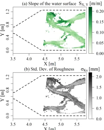
A key parameter for hydraulics and sediment transport is the energy slope S, hereafter considered to be equal to the bed slope following the flow paths SX,Y. Since the flow is generally close to the critical regime in rough and steep streams (Grant 1997; Ghilardi et al. 2014b; Schneider et al. 2015; Ran et al. 2016), it is assumed that no extensive backwater effects occurred, and thus that the free surface is locally adjusted to the slope and roughness and globally parallel to the bed slope. This is a reasonable assumption in steep slopes, as observed by, e.g., Ran et al. (2016), but a possibly excessive assumption in other configurations with gentler slopes or close to structures.

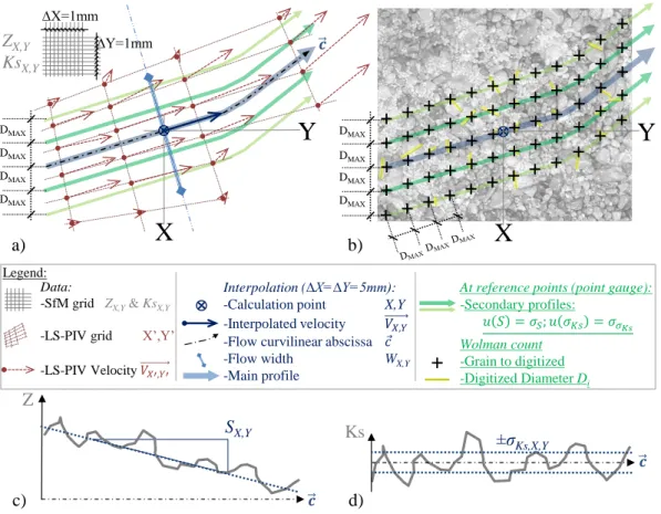
SX,Y was measured at a given position X,Y following several steps summarized here and in Figure 7: 1. The flow direction was extracted from the VX,Y grid;

2. A transversal profile, perpendicular to the flow direction was defined;

3. The flow width WX,Y was defined as the transversal profile length such that V > V0= 0.02 m/s: with V0the

lower limit; defined such that the water depth was negligible;

4. The curvilinear abscissacX,Y~ of the local longitudinal profile axis was defined parallel to the flow direction, i.e., along the surface streamline passing by the point (X, Y ). It had a lenght equal to 3 times WX,Y, a value that was selected after a parametric study: Shorter profiles tended to be excessively affected by local high roughness, while longer profiles tended to leave the flow paths and to be affected by bank topography; 5. A linear fit of the bed elevation ZX,Y along the curvilinear abscissa cX,Y~ defines the local flow slope SX,Y

(Fig. 7c).

Specifically at the reference point locations, additional extractions were performed to quantify the uncertainties (light green arrows in Fig. 7a). Four additional profiles were defined whose slopes were also extracted. The slope uncertainty u(S) at the reference points was considered to be the standard deviation of slope estimates along the five profiles.

The procedure was applied in all flowing areas captured within the LSPIV measurement, determining the flow slope field SX,Y (Fig. 8a).

3.3

Flow roughness proxies

In addition to slope, flow features are fundamentally correlated to bed roughness. The roughness of gravel bed rivers is typically described using a proxy Di, often derived from the grain size distribution of the surface material, usually D50 or D84 (Ferguson 2007). However, the advent of accurate topographical measurement devices has increasingly

resulted in the use of alternative roughness indicators such as the standard deviation of the bed elevation (Aberle and Smart 2003; Nitsche et al. 2012; D’Agostino and Michelini 2015; Schneider et al. 2015; V´azquez-Tarr´ıo et al. 2017). Both approaches were considered here.

Classic GSD measurements were made with the Wolman surface-counting method (Wolman 1954). The counting was also performed precisely along the aforementioned profiles characterizing the reference point vicinity (Fig. 7b): The HD-orthorectified images of the bed surface derived from the photogrammetry analysis were displayed, with marks spaced at DM AX− mm, along the five longitudinal profiles. The smallest diameter of the grain located under each mark was digitally measured on the orthorectified picture of the dry bed.

An average number of 112 ± 45 pebble diameters were digitally measured at each reference point (55–260 pebbles depending on the profile length). The distributions and their quantiles D50 and D84 are proxies of the

local bed roughness. As each digitized point had an accuracy of ±1 pixel and the pixel size was 0.2 mm, the X and Y uncertainties were u(X) = u(Y ) = 0.2 mm at each end of the digitized diameter. The accuracy of the diameter measurement was thus estimated through error propagation to be u(Di) =p(2 × u(X))2+ (2 × u(Y ))2= ±0.57 mm.

The standard deviation of the roughness σKsX,Y was computed along the longitudinal profile of the flow (Fig. 7a & d) at each pixel of the velocity grid (Fig. 8b). In order to quantify the uncertainty of this parameter at the reference points, σKsX,Y was also computed along the secondary longitudinal profiles. The uncertainty of σKsX,Y is considered to be the standard deviation of the five profiles σKsX,Y (Fig. 7b).

Piton

et

al.

(2018)

W

ater

R

esour

ces

R

ese

ar

ch

,

54.

DOI:10.1029/2017WR021314

,

first

author’s

p

ersonal

cop

y

-SfM grid ZX,Y & KsX,Y

-LS-PIV grid X’,Y’ -LS-PIV Velocity 𝑉𝑋′,𝑌′ DMAX DMAX DMAX DMAX ∆Y=1mm ∆X=1mm

Z

Ks

Y

X

a)

b)

Point Gauge Digitalized Di Profile ± 2DMAX

DMAX DMAX DMAX DMAX

±σ

S

Z

-Calculation point X,Y -Interpolated velocity 𝑉𝑋,𝑌

-Flow curvilinear abscissa 𝑐

-Flow width WX,Y

-Main profile

At reference points (point gauge):

-Secondary profiles: 𝑢 𝑆 = 𝜎𝑆; 𝑢 𝜎𝐾𝑠 = 𝜎𝜎𝐾𝑠 Wolman count -Grain to digitized -Digitized Diameter Di

Ks

c)

d)

Y

X

Figure 7: Sketch of the friction law parameters extraction algorithm: a) location of the flow profiles and curvilinear abscissa ~c: parallel to the local velocity interpolated at point X,Y ; b) location of the Wolman count performed at reference points: precisely on the same main and secondary profiles; c) water surface slope SX,Y extraction by a linear fit of ZX,Y along ~c; and d) flow roughness σKsX,Y extraction: standard deviation of KsX,Y along ~c. Parameters underlined in the legend are extracted only at reference points, while data and interpolation parameters are available at least on all of the LSPIV-measured area.

4

Depth reconstruction

4.1

Using a friction law

Friction laws are equations that relate flow velocity to flow depth (or alternatively hydraulic radius or specific discharge, Rickenmann and Recking 2011). Their simplest forms relate the water depth d to the velocity V, flow slope S, and a roughness parameter K through an equation generally given in the dimensionless form:

V √

gdS = f (S, d, K) (1)

with g the gravitational acceleration.

A great number of friction laws could be good candidates for our steep-slope case (see review of D’Agostino and Michelini 2015). Piton (2016, p. 144) tested several of these laws and observed underestimations with both the universally used Manning-–Strickler equation and the Aberle and Smart (2003) equation, theoretically more adapted to steep, rough beds. On the contrary, the variable power equation (VPE) of Ferguson (2007) adapted to both shallow and deep flows was found to provide the best performance. It was thus selected to be used and is the following: V √ gdS = 2.5(d/D84) p 1 + 0.15(d/D84)5/3 (2) Since the inverse of Equation (2), d = f−1(V, S, K), has no obvious explicit form, the computed water depth is

Piton

et

al.

(2018)

W

ater

R

esour

ces

R

ese

ar

ch

,

54.

DOI:10.1029/2017WR021314

,

first

author’s

p

ersonal

cop

y

Figure 8: Friction law parameters: a) Slope of the water surface SX,Y; and b) Roughness standard deviation in the flow direction σKsX,Y (GSD2, Ql=1.7 l/s, t=48 min). Note that since SX,Y and σKsX,Y are computed along flow directions, they are not computed in dry areas (white areas in the figure) although these areas have absolute roughness and slope as seen on Figure 6

Piton

et

al.

(2018)

W

ater

R

esour

ces

R

ese

ar

ch

,

54.

DOI:10.1029/2017WR021314

,

first

author’s

p

ersonal

cop

y

VX,Y pgSX,Y − 2.5(d 3/2 X,Y/D84,X,Y) p1 + 0.15(dX,Y/D84,X,Y)5/3 = 0 (3)

At the 96 reference points, seven points were removed because of uncertain X, Y locations and proximity to intensively sorted areas that induced uncertainties on the roughness. The water depth and D84had been measured,

SX,Y and σKs,X,Y extraction procedures were applied at the 89 remaining reference points and the water depth were reconstructed. The measured water depths can be compared with the computed water depths to test the relevance of Eq. (3).

Fig. 9 shows the statistics of the ratio between computed and measured water depths. The ratio is on average very close to one and underestimations seem to balance overestimations. The statistical performances of this approach and uncertainty propagation are further discussed in paragraph 5.1.

● ● ●

●

VPE(D84): Eq. 3 VPE(σKs): Eq. 5

0

1

2

3

Friction law formulation

dca lc dm ea s ● ● ● ● 1.02±0.53 1.03±0.52

Figure 9: Statistical distribution of the ratio: computed water depth / measured water depth, water depth computed using the Ferguson (2007) form (VPE(D84: Eq. (3)) and the modified Ferguson form (VPE(σKs): Eq. (5)). Numbers below the boxes are mean values and standard deviations, upper circles are outliers higher than 1.5 the interquartile range.

4.2

Comparison of roughness proxies

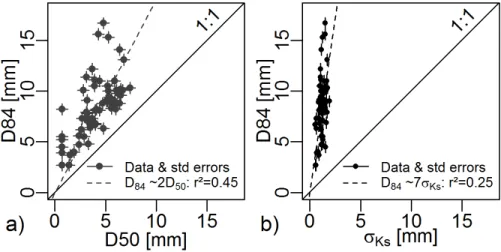
An extension of the depth reconstruction on all of the flowing area is feasible if roughness can be estimated every-where. Both the grain size distribution and the roughness standard deviation were measured along the longitudinal profiles defined at the reference points (Fig. 7). The correlations between these roughness proxies are analyzed in Figure 10.

Piton

et

al.

(2018)

W

ater

R

esour

ces

R

ese

ar

ch

,

54.

DOI:10.1029/2017WR021314

,

first

author’s

p

ersonal

cop

y

D84≈ 7σKs (4)

The correlations relations were chosen to be proportional (Di= A × σKs) rather than linear (Di= A × σKs+ B) so as to simplify the approach, thus creating a simple dimensionless ratio between DX and σKs.

Scattering remains which demonstrates that similar gravel mixtures, i.e., same Di, may have variable granular arrangements, imbrication and interlocking, leading to variable vertical roughness, i.e., different σKs. The fact that there are variably-rough-although-equally-coarse beds is an issue of Di roughness proxies, highlitghted by several authors (Smart et al. 2002; Aberle and Smart 2003; Ferguson 2007). Therefore, we chose to directly measure roughness and to introduce it in the friction law, rather than estimating the surface distribution of grain size D84

using image analysis, like e.g., in the grain sorting study of Leduc et al. (2015). The estimation would additionally be aggravated by new computation steps and thus sources of uncertainties.

4.3

Extension of depth reconstruction to all channels

Since increasing roughness is undoubtedly related to increasing sizes of sediments, σKs can be used directly by introducing Eq. (4) in Eq. (3):

VX,Y pgSX,Y − 2.5(d 3/2 X,Y/7σKs,X,Y) p1 + 0.15(dX,Y/7σKs,X,Y)5/3 = 0 (5)

It is worth stressing that this approach particularly makes sense in friction laws because one is looking for a roughness proxy when using Di (Ferguson 2007). A direct roughness measurement may consequently improve the results as shown here.

The performances of this modified Ferguson equation are also displayed in Figure 9. Equation (5) proved to have equivalent capacity in estimating the water depths than the initial formulation using D84: the median and mean of

the ratio are centered on unity, there are fewer outliers and balanced underestimations and overestimations (Fig. 9). It demonstrates the relevance of using the direct roughness measurement instead of the diameter, despite the relatively low correlation coefficient shown in Fig. 10. This result is consistent with the field analysis of Schneider et al. (2015).

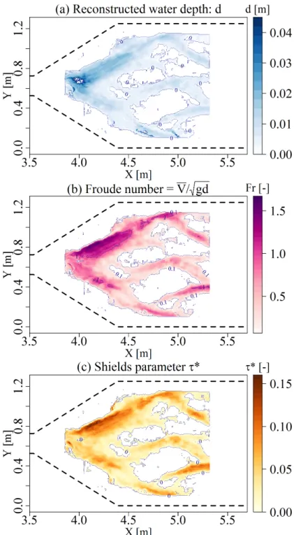
Two-dimensional water depth fields can then be reconstructed by applying the full procedure on the entire LSPIV measurement area (Fig. 11a): (i) velocity measurement and interpolation, (ii) SX,Y and σKs extractions and (iii) application of Equation (5). Other useful flow descriptors can also be mapped as the Froude number (here defined as V /√gd) or the Shields parameter (here defined as = Sd/[(s − 1)7σKs] ≈ Sd/[(s − 1)D84] with the

sediment density s, enabling statistical analysis of the flow features (Fig. 11b & c).

5

Discussion

5.1

Friction law selection and uncertainty propagation

The friction law verification, synthesized here and detailed in Piton (2016, p. 144), proved that the VPE of Ferguson (2007) was the most suitable to our case. This is consistent with the analysis of Rickenmann and Recking (2011) on a large data set comprising well controlled flow conditions, with Schneider et al. (2015) in a steep to extremely steep, heavily-paved stream, or with Recking et al. (2016) for flows over both uniform and poorly sorted beds.

A more detailed look at our validation test shows that at 67% of reference points, dcalc/dmeas is within a range of 0.5–1.5. A performance that is similar or a bit lower compared to the VPE in better controlled conditions. Rickenmann and Recking (2011) for instance obtained scores of 67%, 72%, 91% of velocities in the same range for similar submergence than ours, i.e., with d/D84 = [0;0.7], [0.7;1] and [1;3], respectively. One may be surprised by

such large uncertainties. The reconstructed depths remain nonetheless very interesting in the poorly known context of 10%- to 15%-steep streams with very coarse and mobile beds, where the water depth definition is intrinsically uncertain (Fig. 1) and its measurement always complicated. Special attention must however be given to the quantification and propagation of uncertainties.

Uncertainties may arise from the friction law itself or from the measurements of the input parameters V, S and σKs, as well as from the water depth measurement at the validation step. Approaches for uncertainty estimation were proposed at several steps of the study, often by the standard deviation of repeated measurements. Their

Piton

et

al.

(2018)

W

ater

R

esour

ces

R

ese

ar

ch

,

54.

DOI:10.1029/2017WR021314

,

first

author’s

p

ersonal

cop

y

Figure 11: Maps of inversely computed flow properties: a) water depth d, b) Froude number V /√gd and, c) Shields parameter ≈ Sd/[(s − 1)7σKs] (GSD2, Ql=2.2 l/s, t=25 min)

Piton

et

al.

(2018)

W

ater

R

esour

ces

R

ese

ar

ch

,

54.

DOI:10.1029/2017WR021314

,

first

author’s

p

ersonal

cop

y

On the contrary Eq. (2) was unsuitable for direct analytical uncertainty propagation because no direct analytical expression of the depth, i.e., d = f (V, S, σKs), could be found. A preliminary numerical sensitivity analysis on each parameter showed that, in the typical range of variation of our experimental conditions, an arbitrary 10% uncertainty on V , S and σKs induced 10%, 5% and 6% uncertainties on the depth, respectively. The non linearity of Eq. (2) has indeed the interesting property to either maintain or reduce uncertainty ranges. In order to estimate total uncertainty on depth from compound uncertainties on all parameters, a numerical approach was implemented using the uncertainties of velocities, slopes and roughnesses to compute the resulting water depth uncertainty. A Monte Carlo simulation generated 10,000 values of parameter variations from normal distributions (centred on zero, standard deviation equal to parameter uncertainty). These variations were introduced in Eq. (5) and the corresponding water depths were computed. For each reference point, the water depth uncertainty is considered to be the standard deviation of these uncertain depth samples.

The uncertainty on the reconstructed water depth at the 89 reference points was on average 2 mm in absolute, i.e., 15% relatively to the measured value. This parameter-related 15% uncertainty weights thus less than the uncertainty coming from the use of the friction law itself which is higher – about ±50% – as discussed above. The depth reconstruction procedure is consequently quite robust to uncertain parameters. This reanalysis is also an opportunity to stress that friction laws remain only partially accurate and improving them deserves research efforts. It is also worth stressing that the depth measurement, that is used as reference, is also uncertain at ±50% (±5.3 mm). However, Piton (2016, p. 147) showed that uncertainties on depth measurement and on depth reconstruction likely do not cumulate and partially compensate each other.

Finally one must stress that application of the method is limited to flow conditions where the shallow water equations apply and flows are relatively closed to uniform flows. Only relatively and not strictly because Eq. (2) is quite stable to uncertain slope values as discussed previously. Configuration with marked backwater effects, where energy slopes strongly deviate from bed slopes, are not favorable in the present version of the procedure, although the improvements discussed in the next sections could make such configurations measurable.

5.2

Horizontal flow surface assumption

The horizontality of the free surface is implicitly assumed in the usual LSPIV technique, which is reasonable in most laboratory applications (e.g., Fujita et al. 1998; Kantoush et al. 2011). Recent applications in steep slope contexts addressed the possible bias resulting from an excessively steep free surface (Le Boursicaud et al. 2016; Ran et al. 2016; Stumpf et al. 2016) or from 3D flow patterns related to obstacles (bridge piers, protruding boulders, Dramais et al. 2011). To solve this problem, Ran et al. (2016) performed stereo-picture acquisitions and computed the free surface as a bidimensional plane with a variable slope. In the same vein, Dramais et al. (2011) used the simple alternative to orthorectify the fast camera pictures in the flume plan rather than horizontally. It is then possible to compute the velocity in this local referential system, and to later retrieve these results in a vertical referential system. A more complicated and rigorous 3D flow analysis could be performed by projecting the flow pictures on the DEM and tracking the pattern correlation on this 3D surface. These improvements are beyond the scope of this work.

5.3

Improving flow depth measurements

Determination of the suitable friction law to use in the procedure is a key step. The reference depth measurements used in this work have uncertainties that lead us to cautious conclusions on the reconstructed flow fields. In future, for similar flow depth reconstruction, the use of more precise techniques for reference depth measurement for the friction law validation step is recommended. Providing that the water surface must be dyed and seeded with black patterns, measuremet of its elevation is possible using photogrammetry, as with the bed surface.

The technical challenge would then be to take enough pictures of the flume at exactly the same time so as to capture an instantaneous image of the flow surface with its patterns. It would require several cameras and, according to dynamic photogrammetry monitoring of avalanches (Pulfer et al. 2013) and torrential flows (Ran et al. 2016), the use of accurate remotely-controlled camera triggering.

This image acquisition would optimally be carried out simultaneously with the LSPIV measurement. The flow must subsequently be stopped, as quickly as possible, to prevent bed geometry and roughness adjustments between the flow measurement and its representative bed measurement. Using such a technique would theoretically enable surface-flow DEM computation. The spatial distribution of water depths would then be computed by subtracting the bed DEM, providing that bed changes between both measurements are reasonably small.

Piton

et

al.

(2018)

W

ater

R

esour

ces

R

ese

ar

ch

,

54.

DOI:10.1029/2017WR021314

,

first

author’s

p

ersonal

cop

y

then be greatly extended, confirming the method’s robustness and giving additional information on its accuracy and bias. It would eventually also enable the development of new and more accurate friction laws based on new flow, topography, and roughness proxies.

5.4

Streamline tracking

Friction laws are basically closure equations of the Bernoulli equation that express the evolution of the flow energy along stream lines, i.e., along lines tangential to the velocity vectors (Lencastre 1983). The slope and roughness parameters should thus be computed along the streamlines. Surface streamlines can be computed from surface velocity measurements (e.g., Willert and Gharib 1991). Assuming that secondary currents are negligible compared with horizontal flow patterns (a reasonable assumption in the context of applying the shallow water equation, Muste et al. 2004), surface streamlines are an interesting proxy of the mean local flow directions.

In a narrow flume or along a given river reach, the streamlines are assumed to follow the main direction of the flume or river. Conversely, in 2D flow computations or reconstructions, flow directions are not systematically parallel to the average flume/river direction. In our case, they are locally diverging, converging, and wandering over the deposit. As discussed previously, the slope and roughness estimations were thus not computed along the flume direction (X-direction in our case) but on local longitudinal profiles, defined parallel to the flow direction (an initial step toward a streamline computation). The procedure is assumed to be reasonably correct as long as the flow curvature radius is small compared with the flow width (which has been validated visually on our data). For highly meandering flows with a curvature radius of the order of magnitude of the flow width, the procedure may fail and the σKs and S extractions should be made along the curved streamlines rather than along profiles locally parallel to the stream line.

5.5

Surface velocity correction

A regularly discussed hypothesis of LSPIV works is the use of a constant velocity index α=0.85 between the surface velocity and the depth-averaged velocity. The α parameter fundamentally depends on the vertical velocity profile (Le Coz et al. 2010), which itself varies depending on the flow aspect ratio, micro and macro-roughness, Froude and Reynolds numbers, and macro-roughness relative submergence (Muste et al. 2010). Polatel (2006, p. 39) undertook a comprehensive study of the α variation depending on flow velocity and macro-roughness sizes in a 1D flume, tested with a smooth bed and with a bed covered by flume-wide obstacles (rectangular ribs and simplified dunes). Her experimental conditions covered a range of relatively low submergence (d/macro-roughness vertical size = 3-10), with subcritical flows (F roude = 0.39 − 0.51), and resulted in a fairly small α-range of variation: 0.88 ± 0.04 (mean ± σ; envelop: 0.80-0.94 ). Such values are typical of uniform flows (Costa et al. 2006; Le Coz et al. 2010), even for higher submergence: Legout et al. (2012) and Stumpf et al. (2016) measured α =0.8-0.9 and =0.84-1, on experiments of very shallow overland flows on steep, rough surfaces and a steep, boulder-paved river, respectively. Other authors argue that α may slightly decrease with the submergence AFNOR (2009) and Dramais et al. (2011). The extensive analysis of Welber et al. (2016) highlights the key influence of the roughness submergence on α, but they also conclude that ”α=0.85 is a valid default value” as a spatial average. However, locally, the scatter is huge in non-uniform flows, e.g., in their measurement on the Tagliamento (braided gravel-bed river, Italy).

Similar works addressing near-critical and super-critical flows, as well as even lower submergence down to d/Ks ≈ 1, and with sediment transport, are, however, still lacking – an issue regularly mentioned in the literature (Le Coz et al. 2010; Dramais et al. 2011; Ran et al. 2016; Welber et al. 2016). It would possibly lead to different results than those acquired by Polatel (2005), since two-layer flows (a slow sub-layer under macro-roughness height, below a faster layer overflowing the macro-roughness, Aguirre-Pe and Fuentes 1990), are expected in steep rough channels. Additional modifications of the flow profile may emerge from feedback related to sediment transport (Recking et al. 2008b; Revil-Baudard et al. 2015).

6

Conclusion

The present work describes a measurement procedure that takes advantage of the recent development of affordable HD cameras and of user-friendly image analysis software. This procedure could be extended to other experimental conditions, including field studies, and seems promising considering that: (i) it is relatively simple to implement, and (ii) the necessary equipment is quite affordable: cameras and a photogrammetry software. Using HD images of the

Piton

et

al.

(2018)

W

ater

R

esour

ces

R

ese

ar

ch

,

54.

DOI:10.1029/2017WR021314

,

first

author’s

p

ersonal

cop

y

of deposit thickness, slope S, roughness σKs, and velocity V at unprecedented spatiotemporal resolution. Care was taken to measure the slope and roughness along the flow directions which, in freely adjusting beds, are often not the main flume direction. Piton (2016, p. 147) demonstrated the relevance of using the Ferguson (2007) variable power equation (Eq. 2) as a friction law in gravel bed flows. Using seven times the local standard deviation of the bed roughness σKsas a proxy of the D84parameter in the Ferguson (2007) friction law, it was be possible to extend

the water depth computation by inverting the friction law (d = f−1(V, S, σKs)) throughout the entire flooded area. Complete spatial distribution of the flow features (flow slope, roughness, depth average velocity, and depth) can be reconstructed, thus providing numerous data on these freely adjusting systems, currently still poorly known. The method is simple in essence and relatively affordable regarding the amount of data it can produce. The authors hope that it will be tested and improved in other experimental situations and help expand our understanding of the dynamics of freely adjusting geophysical flows.

Acknowledgments The data and code used in this study are available as supplementary material with the paper, it enables to generate Fig. 5, 6, 8 and 11 and their counterparts for both flowing configurations displayed in Fig. 4. This study was funded by Irstea, the INTEREG-ALCOTRA European RISBA project, the ALPINE SPACE European SEDALP project and the H2020 project NAIAD [grant no. 730497] from the European Union’s Horizon 2020 research and innovation programme. The authors would like to thank Benoˆıt CAMENEN for the idea of using Fudaa-LSPIV, Guillaume NORD and C´edric LEGOUT for the TiO2 trick, Jules LE GUERN, Costanza

CARBONARI, S´egol`ene MEJEAN, Firmin FONTAINE and Coraline BEL for their help in the experimental setup development and experience work, as well as the AE Mar´ıo FRANCA, Volker WEITBRECHT, Yulia AKUTINA and two other anonymous reviewers who greatly helped us by providing thorough and helpful remarks on previous drafts of this paper.

References

Aberle, J. and Smart, G. (2003). “The influence of roughness structure on flow resistance on steep slopes”. English; French. Journal of Hydraulic Research 41.3, pp. 259–269. issn: 00221686.

AFNOR (2009). NF EN ISO 748 - Hydrom´etrie Mesurage du d´ebit des liquides dans les canaux d´ecouverts au moyen de d´ebim`etres ou de flotteurs. (in French).

Agisoft LLC (2014). Agisoft PhotoScan User Manual - Professional Edition, Version 1.1. 85p. Agisoft LLC. Aguirre-Pe, J. and Fuentes, R. (1990). “Resistance to flow in steep rough streams”. Journal of Hydraulic Engineering

116.11, pp. 1374–1387. issn: 07339429.

Brasington, J., Vericat, D., and Rychkov, I. (2012). “Modeling river bed morphology, roughness, and surface sed-imentology using high resolution terrestrial laser scanning”. Water Resources Research 48.11. doi: 10.1029/ 2012wr012223.

Cao, H. H. (1985). “R´esistance hydraulique d’un lit de gravier mobile `a pente raide”. PhD thesis. EPFL Lausanne. Costa, J., Cheng, R., Haeni, F., Melcher, N., Spicer, K., Hayes, E., Plant, W., Hayes, K., Teague, C., and Barrick, D. (2006). “Use of radar to monitor stream discharge by noncontact methods”. Water Resources Research 42, pp. 1–14.

D’Agostino, V and Michelini, T (2015). “On kinematics and flow velocity prediction in step-pool channels”. Water Resources Research 51.6, pp. 4650–4667. doi: 10.1002/2014WR016631..

Detert, M. and Weitbrecht, V. (2015). “A low-cost airborne velocimetry system: proof of concept”. Journal of Hydraulic Research 53.4, pp. 532–539. doi: 10.1080/00221686.2015.1054322.

Detert, M., Johnson, E. D., and Weitbrecht, V. (2017). “Proof-of-concept for low-cost and non-contact synoptic airborne river flow measurements”. International Journal of Remote Sensing 38.8-10, pp. 2780–2807. doi: 10. 1080/01431161.2017.1294782.

Dramais, G., Le Coz, J., Camenen, B, and Hauet, A. (2011). “Advantages of a mobile LSPIV method for measuring flood discharges and improving stage-discharge curves”. Journal of Hydro-environment Research 5/4, pp. 301– 312.

Ferguson, R. (2007). “Flow resistance equations for gravel-and boulder-bed streams”. Water Resources Research 43.5, pp. 1–12. doi: 10.1029/2006WR005422.

Frey, P., Tannou, S., Tacnet, J., Richard, D., and Koulinski, V. (1999). Interactions Ecoulements torrentiels -Ouvrages terminaux de plages de d´epˆot [Interactions between torrential flows and open check dams]. Tech. rep. (In French). Pˆole grenoblois d’Etudes et de Recherche pour la pr´evention des risques naturels.

Piton

et

al.

(2018)

W

ater

R

esour

ces

R

ese

ar

ch

,

54.

DOI:10.1029/2017WR021314

,

first

author’s

p

ersonal

cop

y

Ghilardi, T, Franca, M., and Schleiss, A. (2014a). “Bulk velocity measurements by video analysis of dye tracer in a macro-rough channel”. Measurement Science and Technology 25.3, pp. 1–11.

Ghilardi, T., Franca, M. J., and Schleiss, A. J. (2014b). “Bed load fluctuations in a steep channel”. Water Resources Research 50.8, pp. 6557–6576.

Grant, G. (1997). “Critical flow constrains flow hydraulics in mobile-bed streams: A new hypothesis”. Water Re-sources Research 33.2, pp. 349–358. issn: 00431397.

Hauet, A., Jodeau, M., Le Coz, J., Marchand, B., Die Moran, A., Le Boursicaud, R., and Dramais, G. (2014). “Application of the LSPIV method for the measurement of velocity fields and flood discharges in reduced scale model and in rivers [Application de la m´ethode LSPIV pour la mesure de champs de vitesse et de d´ebits de crue sur mod`ele r´eduit et en rivi`_{ere]”. French. Houille Blanche 3, pp. 16–22. issn: 00186368. doi: 10.1051/lhb/} 2014024.

Heller, V. (2011). “Scale effects in physical hydraulic engineering models”. Journal Of Hydraulic Research 49.3, pp. 293–306. issn: 0022-1686. doi: 10.1080/00221686.2011.578914.

Ishikawa, Y, Osanai, N, Koizumi, Y, Takezaki, S, and Matsumura, K (1996). “A method of planning and designing sediment retarding basins”. INTERPRAEVENT Conference Proceedings.

JCGM (2008). Evaluation of measurement data — Guide to the expression of uncertainty in measurement. Tech. rep. JCGM 100:2008. 120p. Joint Committee for Guides in Metrology.

Jerolmack, D. and Paola, C. (2010). “Shredding of environmental signals by sediment transport”. Geophysical Research Letters 37.19, pp. 1–5. issn: 00948276. doi: 10.1029/2010GL044638.

Jodeau, M., Hauet, A., Paquier, A., Le Coz, J., and Dramais, G. (2008). “Application and evaluation of LS-PIV technique for the monitoring of river surface velocities in high flow conditions”. Flow Measurement and Instrumentation 19.2, pp. 117–127. doi: 10.1016/j.flowmeasinst.2007.11.004.

Kantoush, S. A., Schleiss, A. J., Sumi, T., and Murasaki, M. (2011). “LSPIV implementation for environmental flow in various laboratory and field cases”. Journal of Hydro-environment Research 5.4, pp. 263–276.

Le Boursicaud, R., P´enard, L., Hauet, A., Thollet, F., and Le Coz, J. (2016). “Gauging extreme floods on YouTube: Application of LSPIV to home movies for the post-event determination of stream discharges”. Hydrological Processes 30.1, pp. 90–105.

Le Coz, J., Hauet, A., Pierrefeu, G., Dramais, G., and Camenen, B. (2010). “Performance of image-based velocimetry (LSPIV) applied to flash-flood discharge measurements in Mediterranean rivers”. Journal of Hydrology 394, pp. 42–52.

Le Coz, J., Jodeau, M., Hauet, A., Marchand, B., and Le Boursicaud, R. (2014). “Image-based velocity and discharge measurements in field and laboratory river engineering studies using the free FUDAA-LSPIV soft-ware”. Proceedings of the International Conference on Fluvial Hydraulics, RIVER FLOW 2014, Lausanne: CRC Press/Balkema, pp. 1961–1967. isbn: 9781138026742.

Le Guern, J. (2014). “Msc. Thesis manuscripts: Mod´elisation physique des plages de d´epˆot : analyse de la dynamique de remplissage [Small scale model of sediment traps: filling dynamic analysis]”. Univ. Fran¸cois Rablais - Tours / Laboratoire IRSTEA - Grenoble (In French). MA thesis.

Leduc, P, Ashmore, P, and Gardner, J. (2015). “Grain sorting in the morphological active layer of a braided river physical model”. Earth Surface Dynamics 3.4, p. 577. doi: 10.5194/esurf-3-577-2015.

Legout, C., Darboux, F., N´ed´elec, Y., Hauet, A., Esteves, M., Renaux, B., Denis, H., and Cordier, S. (2012). “High spatial resolution mapping of surface velocities and depths for shallow overland flow”. Earth Surface Processes and Landforms 37.9, pp. 984–993. issn: 01979337. doi: 10.1002/esp.3220.

Lencastre, A. (1983). Hydraulique g´en´erale. (In French). Paris: Eyrolles, p. 633.

Maas, H., Gruen, A., and Papantoniou, D. (1993). “Particle tracking velocimetry in three-dimensional flows”. Experiments in Fluids 15.2. doi: 10.1007/bf00190953.

Muste, M., Fujita, I., and Hauet, A. (2010). “Large-scale particle image velocimetry for measurements in riverine environments”. Water Resources Research 46.4, pp. 1–14. issn: 00431397. doi: 10.1029/2008WR006950. Muste, M., Hauet, A., Fujita, I., Legout, C., and Ho, H.-C. (2014). “Capabilities of Large-scale Particle Image

Velocimetry to characterize shallow free-surface flows”. Advances in Water Resources 70, pp. 160–171. doi: 10.1016/j.advwatres.2014.04.004.

Muste, M., Xiong, Z., Sch¨one, J., and Li, Z. (2004). “Validation and extension of image velocimetry capabilities for flow diagnostics in hydraulic modeling”. Journal of Hydraulic Engineering 130.3, pp. 175–185.