Investigation of Molikpaq
1986 Ice Loading Events &
Evaluation of Load Measuring
Devices
FINAL REPORT
Submitted to:
Canadian Hydraulics Centre
National Research Council of Canada
Ottawa, ON
Canada K1A 0R6
By:
Ian Jordaan and Associates Inc. 7 East Middle Battery Road St. John’s, NL
Investigation of Molikpaq 1986 Ice Loading Events
& Evaluation of Load Measuring Devices
Final Report
Submitted to:
Canadian Hydraulics Centre
National Research Council of Canada
Ottawa On
Canada K1A 0R6
Submitted by:
Ian Jordaan & Associates
7 East Middle Battery Road
St John’s NL
Canada A1A 1A3
Jonathon Bruce, C-CORE Mark Fuglem, C-CORE
Executive Summary
The project focuses on the measurements of load on the Molikpaq structure during the 1986 deployment at the Amauligak I65 location. The structure consists of a steel annulus, octagonal in form, serving as a caisson to support drilling operations. The structure was instrumented so as to obtain estimates of ice loads. These have been based on Medof panels attached to the outer steel surface, strain gauges installed on the steel structure, extensometers measuring the deformation of the caisson as well as inferences from the geotechnical design and performance of the structure. In past work, there has been a tendency to use the Medof panels to estimate loads, but at the same time, discrepancies have been noted over the years. In particular, Kevin Hewitt has drawn attention to the fact that geotechnical information suggests lower loads than those estimated from the Medof panels using the original calibrations of these panels. According to Hewitt, the difference could be as high as 300 MN (500 MN as compared to about 200 MN). Subsequent to the ice loading events of 1986, a Joint Industry Project was carried out to study the events and associated measurements of the Molikpaq. This is referred to as the “1986 JIP”. The measurements on the Molikpaq together with the 1986 JIP and its original set of reports have formed the basis of the present study. The IJA project team has concluded that the results of the 1986 JIP need reconsideration. The key aspect that should be reconsidered is the strong reliance on the original calibrations of the Medof panels in the 1986 JIP. The recent report by Klohn Crippen Berger (2009) provides a summary of this JIP. The team is consequently in disagreement with the Klohn Crippen Berger interpretation, which is closely aligned with the 1986 JIP reports. It is considered that the arguments in the report supporting the original Medof calibration are not well-founded.
The IJA project team has acknowledged that there are uncertainties in the Sandwell structural stiffness finite element results (used in conjunction with displacements
measured by extensometers in the present study to provide an alternative estimate of ice loads on the Molikpaq structure), but these are outweighed by the far greater uncertainties in the Medof panel results. In fact, the points raised by Klohn Crippen Berger have been dealt with in our work. The ice mechanics in the report omits reference to work after the 1986 JIP in which the behaviour and failure of high-pressure zones have been discovered. The ice mechanics, as a result, are out of date. No cause to change the present approach has been found in the Klohn Crippen Berger report.
The extensometer readings have also been found to give lower loads than those deduced from the Medof panels, and in some reports, there is an indication that strain gauges have also given low values. This is broadly in agreement with the geotechnical information summarized in the first paragraph above. The supposition in the present study was that probabilistic averaging of local loads might explain part of these differences, at least between the extensometers and the Medof panels. The averaging technique takes into account the fact that for many failure modes, crushing in particular, the spatial variation of pressures across the face of the structure is highly uncorrelated, except locally. This
means that the standard deviation of global loads is much less than that for the locally measured loads (or pressures).
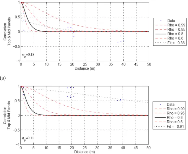
The data from the Medof panels on the Molikpaq were subjected to statistical analysis to determine the variation of correlation with distance. This was carried out for creep and crushing events. The values of the correlation coefficient were used in an analysis to account for the averaging effect, resulting in a model of probabilistic averaging. Then the events were analyzed to determine the effect of probabilistic averaging, as compared to linear (or simple) averaging. The latter is based on extrapolation of the averaged Medof panel loads to the full structure width by the ratio of structure width to Medof panel total width. It is noted that the Medof panel width is about 10% of the structure width.
Results are shown in the following table, where LA = linear averaging and PA =
probabilistic averaging. The values are face loads, but are not given dimensions because of the uncertainty in the Medof panel calibration constant (the original calibration was used). Although reduced global ice loads were found, probabilistic averaging had little effect on creep loads (as expected) but a greater effect in the case of crushing ice failures. The reduction in load was of the order of 15-20%. This was not enough to account for the differences in load estimates noted above.
LA LA PA PA
No Bottom Uniform No Bottom Uniform
Mar-25-N-1 Creep 103.1 103.1 101.9 101.9 Apr-12-E-1 Crushing 168.6 168.6 139.1 139.1 Apr-12-E-2 Crushing 187.5 374.5 158.2 319.6 Apr-12-E-3 Crushing 83.9 92.1 73.3 82.4 May-12-N-1 Crushing 168 343.9 140.9 295.9 May-22-N-1 Creep 108.4 140.3 107.4 139.2 May-22-N-2 Crushing 123.1 213.8 103.2 180.1 Jun-02-E-1 Crushing 127.7 128.9 113.9 115.8 Jun-02-E-2 Creep 86.3 87.2 84.8 85.8
Maximum Nominal Load Maximum Nominal Load
Event Failure Mode
In the table, an adjustment has been made for the fact that in some cases, loads were measured on the lower Medof panels. These did not cover the same lateral width as the main set of panels, in fact were only present on one set of Medof panels per face. The term “Uniform” in the table is a method of allowing for the fact that the lower Medof panel is present for only one set of Medof panels, using a linear extrapolation. The “No Bottom” results do not account for bottom panel loads. Another method, the Ratio method, extrapolates on the basis of the ratio of the lower Medof load to the other loads above it. Neither of these methods (Uniform or Ratio) is satisfactory, particularly for ice crushing. The ice failure process consists of high-pressure zones generally concentrated near the centre of the ice sheet, with occasional excursions towards the edges. Both methods fail to recognize this, and generally overestimate the face loads. It is considered
A review has been conducted of the load measuring devices. The strain gauges have been calibrated to the Medof panel loads in the past, as have the extensometers. The strain gauge readings correlate well with the Medof panel loads, but the calibration factor varies considerably. The figure below, based on the data from all S09 strain gauges, shows the uncertainty in calibration factor (CF). Some differences can be explained by differences in structural details but individual gauges show substantial variation, and taken overall, the figure gives a reasonable illustration of the uncertainty. The variance in the
calibration factor results from the fact that the same strain can be achieved in the gauge from a multitude of local ice loads at various positions and intensity.
An investigation into the past recalibrations of the Medof panels at the Tarsuit location (Tarsiut Island Research Program, 1982-3) has been undertaken. This led to the
conclusion that softening of this material has very likely taken place. The conclusion is reinforced by the very high variability of stiffness in the calibration reports indicating variability in manufacturing quality. In addition there was evidence of softening in the recalibrations and under repeated loadings.
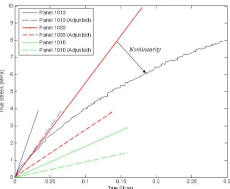
A review was undertaken of the behaviour of the polyurethane material used as part of the construction of the Medof panels. The panels were composed of two parallel steel plates with Adiprene L100 urethane buttons sandwiched between the plates. The outside plate had a thickness of 12.5 mm (1/2") while the Adiprene L100 buttons had a thickness of 2.54mm (1/10”) and a diameter of 9.5 mm (3/8") while the back plate had a thickness of 4.5mm (0.179in). This was in contact with the hull of the structure and welded to it. The urethane buttons were closely spaced at 12.7 mm (1/2") centre to centre, and carried most of the load from the outer surface to the structure.
The original calibration was carried out at a maximum nominal stress on the panel of about 1.86 MPa, resulting in a maximum stress on the polyurethane buttons of about 4 MPa. These stress levels, if uniformly distributed over the panel, might lead to acceptable performance, possibly with small damage or nonlinearity in the material. At the same time, creep is significant for longer term loadings. The original calibrations did not show nonlinearity but nonlinearity was identified in later work by Spencer. In all cases, the stress levels were too low to identify any softening, and none of the programs included meaningful repeated-load tests. A viscoelastic model was developed by Spencer based on his tests, but this is applicable only to low stress levels and one-time loading. The Medof
Ice crushing in particular and mixed-mode failure involve highly localized pressures, so that the pressures are significantly amplified over regions of the panel under these ice failure modes. Crushing in particular will apply loadings akin to “panel beating” with repeated and randomly placed high-pressure zones across the face of the panel. In the literature, and particularly the work of Qi and Boyce, it is found that the stress and strain under plausible conditions for the Medof panels, reached levels that would result in nonlinearities in stress-strain behaviour and in softening associated with the Mullins effect. Further, in most instances, the loads were repeated in many cycles, which would add to the softening effect.
Many results have in the past been premised on the basis that the Medof panels are strictly correct. The analysis in this report shows this to be a questionable assumption as a result of possible softening of the panels. Data gathered using other instruments may form a better basis of load estimation. The following hypotheses were proposed in this work for consideration.
1. The Medof panels form the basis of load estimation, with other devices calibrated to them.
2. The extensometer readings form the basis of load estimation, with other devices calibrated to them.
3. The strain gauges form the basis of load estimation, with other devices calibrated to them.
4. A best estimate compromise between the three estimates form the basis of load estimation.
Our evaluation based on the evidence is that the extensometers form the best method of calibration (item 2 above), with a much higher credibility than the other devices. It is a reasonable conclusion that the Medof panel calibrations changed with time, in the sense of a softening process, giving readings that indicated higher loads than previously thought. The errors are of the order of magnitude two.
It is accepted generally that hydraulically placed sand pumped through a pipeline is loose and not dilative (see Hewitt, 2009), and furthermore, prone to liquefaction. While there are disagreements as to the precise state of the sand core, the estimates based on a loose fill agree in essentials with our current estimates of load. In general terms: our advice from Ryan Phillips is that the three significant load events (March 7/8, April 12, and May 12) exceeded the “basal shear resistance” (say 140 to 180 MN), “but not by very much” (C-CORE Technical Memorandum, July 14, 2009). Our current best estimates of global load for these events based on the extensometer readings are somewhat less than 180 MN (120-160 MN) except for the April 12 event which is greater (about 235 MN). The decelerating floe analysis suggests that the load in the May 12 event might be substantially less than 180 MN, but other estimates are closer to this value. The
geotechnical estimates fall more in line with these values and all estimates are beginning to fall into the same “ballpark”.
The Medof panels have been used for the calibration of the correlation model used for probabilistic averaging. If panels have softened, the correlation structure should remain unchanged, even if different softening of two panels has occurred. If two panels softened in a significantly different way during a loading event, this might have some effect on the correlation analysis. But this scenario is unlikely since most of the softening would have occurred in the early stages of loading, in the 1984-5 season or early in the 1985-6 season, and the change thereafter not very rapid.
The main factors affecting the choice of stiffness are: 1. core stiffness, and
2. proportion and distribution of load on the base and the consequent load path. It is difficult to obtain a definitive estimate of the structure stiffness from the Sandwell report for use with the extensometer readings. In our calibration work, the values of stiffness (Load Distortion Ratio) equal to 2.2, 2.6 and 3.0 MNmm–1 have been chosen. Our best estimate is of the order of 2.6 MNmm–1 but the surrounding uncertainty has been taken into account by using a range of values. The values just quoted are for face loads. In the case of global loads, the inclusion of a lateral force in the Sandwell analysis of the forces on the corners tends to make the structure stiffer than it is in reality. As a result, the load distortion ratios for global loads would tend to be too high and exaggerate them.
The loading pattern in the loading case under consideration must be carefully considered in choosing the appropriate factor. A methodology based on matrix methods for dealing with biaxial loading and superposition on multiple faces has been developed successfully, but does suffer from difficulties in the calibration based on the Sandwell report
mentioned in the preceding paragraph.
A new finite element analysis with well chosen boundary conditions would be most useful.
In the following, a summary is presented of the main conclusions of the analysis of the three selected events, as decided by clients in the June, 2008 meeting.
May 12th Floe Deceleration Event
The event of May 12th, in which a large floe in open water impacted the Molikpaq, presented a unique opportunity to assess independently the stiffness of the Molikaq in terms of global load versus extensometer readings. Because the floe was in open water, and the size and velocity of the floe were provided, the initial kinetic energy of floe can be estimated. Assuming that the load during the interaction is proportional to the north-south ring distortion and assuming a linear response, the stiffness (in MN applied force per mm ring distortion) required so that the floe stops in the observed time can be calibrated. The necessary global stiffness (load distortion ratio) is 2.2 MNmm-1,
distortion ratio (2.6 MNmm-1) results in a load of 123 MN. This is a face load, and in the present event the loading was mainly concentrated on the north-east face of the structure. A sensitivity analysis of uncertainty in the time during which the floe deceleration proper occurred, was undertaken. To do this, the first 12 minutes of the impact was removed. The contribution for these first 12 minutes appears to correspond to small loads based on the extensometer ring distortion. It was assumed that the floe stopped in 15 minutes as opposed to the 27 minute approach described previously. A structural stiffness of 2.9 MNmm-1 with a maximum global load of 130 MN is the result of this analysis. The matrix model has also been applied to the May 12, 1986 data set. Using this approach a global load estimate of 126 MN results. This approach considers the predominant loading on the North face in addition to the loading occurring on the North East and East faces. In reality, the load seems to have been mainly a face load so that this is likely to be an overestimate.
The deceleration analysis supports the case that ice loads have been overestimated, giving grounds for using significantly lower stiffness values (load distortion ratios).
Analysis of March 25 Event
On March 25th, there were two significant creep loading ice events which were analyzed. For the first event, a face load of 34 MN was obtained, with a value of 55 MN in the second. The second creep event from March 25 was considered in further detail to examine the reasons for the bilinear slope between the Medof loads and ring distortions and the apparent hysteresis effect. By plotting the Medof column loads against ring distortion for given loading and unloading cycles of the north face, it is seen that there is first loading on the east side of the north face, then the west side and finally the center. The difference in loading times may result from the direction of ice movement and the observed fact that in creep type loads, loading occurs at the edges of a face before the center. The net effect is to produce an apparent bilinear slope in the curve giving total Medof load as a function of ring distortion. The analysis also showed that there were considerable differences in the Medof loads for adjacent columns, and that the non-zero intercepts for the Medof load versus ring distortion may be a function of differences in the time of loading and the fact that only 10% of the face was instrumented.
Analysis of March 7th Event
On March 7th there were two significant events which were considered. The ice came from the North impacting the North, North West and West faces. Due to the loading being on the West face, there were no Medof panels to consider. As a result of there being loading on more than one face, the method of calibrating Medof loads on the North face to the face load determined from the N-S ring distortion was not successful. The matrix method was also used as this has the capability of using extensometer ring distortions from multiple faces. The result was very sensitive to the initial offsets which
determined by the extensometers for various ring distortion ratios chosen based on the results presented by Sandwell (1991). The Medof panel loads include appropriate averaging.
0325A 25-Mar-86 f603250801 34 MN 0.27 0.32 0.37
0325B 25-Mar-86 f603251302 55 MN 0.44 0.52 0.60
0512A 12-May-86 f605120301 123 MN 0.44 0.52 0.60
0307A 7-Mar-86 f603071520 100 MN N/A N/A N/A
0307B 7-Mar-86 f603071603 81 MN N/A N/A N/A
Factor used to reduce the Medof panel face load to account for softening
Ring Distortion Ratio = 2.2 Ring Distortion Ratio = 2.6 Ring Distortion Ratio = 3.0
Note: Those events with N/A were events for which this method was considered to be inappropriate as there was load on multiple faces and limited contact with Medof panels. The matrix method was adopted for these cases.
Event
Number Date Fast File
Max Face Load for 2.6 MN/mm Ring Distortion Ratio
With regard to the matrix method, the authors feel that the method is promising, and could be much improved by more work on zeroing, and by adjustments to the stiffness matrix.
While there are disagreements as to the precise state of the sand core, the estimates based on a loose fill agree in essentials with our current estimates of load. In general terms: our advice from Ryan Phillips is that the three significant load events (March 7/8, April 12, and May 12) exceeded the “basal shear resistance” (say 140-180 MN), “but not by very much” (C-CORE Technical Memorandum, July 14, 2009). The state of the core would also be affected by the dynamic shaking during these events. Our current best estimates of load for these events based on the extensometer readings are somewhat less than 200 MN except for the April 12 event which is somewhat greater. The decelerating floe and other analyses suggest that the load in the May 12 event is less than 140 MN. But the geotechnical estimates are beginning to fall into the same “ballpark” as other estimates. In the absence of a correction for Medof panel softening, the trends of the Molikpaq data are not consistent with the other data. Figure A below, with power-law trendlines
illustrates the discrepancy. Accounting for panel softening yields results that are much more consistent with those observed from the STRICE, JOIA and Cook Inlet datasets. Based on a comparison with other data sets, it has been concluded that a panel of constant width experiences decreasing pressure over the loaded area for increasing ice thickness. This is consistent with the well known pressure-area scale effect for ice.
The main conclusion of the work is that design pressures based on the Medof panels attached to the Molikpaq structure, for the 1985-86 deployment, overestimate the loads by about 50%. The more detailed approach based on probabilistic methods, given in our Appendix IJA – A, should also be adjusted to give appropriate input values. The
methodology for local pressures, as analyzed in the paper (Jordaan, Bruce, Masterson and Frederking, 2010, Cold Regions Science and Technology, in press) based on the Medof panels, is also relevant for this future work.
STRICE and Molikpaq Column Mean Pressure vs. Ice Thickness Data 0 0.2 0.4 0.6 0.8 1 1.2 0.3 0.4 0.5 0.6 0.7 0.8 Ice Thickness (m) M e a n I c e P res sure (M P a ) Molikpaq Data STRICE Data
Power (Molikpaq Data) Power (STRICE Data)
Table of Contents
1 Background and Motivation ... 1-1
1.1 The Molikpaq Structure... 1-1 1.2 Use of Ice pressures in Design... 1-3 1.3 Fundamental Questions and Approach... 1-3 1.4 Velocity Effects... 1-4 1.5 Definition of an Event: Data Files... 1-5 1.6 Geotechnical Aspects and Klohn Crippen Berger (2009)... 1-8 1.7 Face Load versus Global Loads; Pressures... 1-8 1.8 Organization of the Present Study... 1-11
2 The Structural Behaviour of the Molikpaq... 2-1
2.1 Deformations of the Structure... 2-1 2.2 Boundary Conditions... 2-1 2.3 Finite Element Analyses... 2-3 2.4 Sandwell (1991) Report... 2-3 2.4.1 Shell International Finite Element Analysis... 2-9 2.4.2 Conclusions Regarding Structure Stiffness and Extensometer Calibration for Face Loads... 2-9 2.5 Matrix Solution for Biaxial Loading... 2-10 2.6 Conclusions... 2-16 3 Instrumentation... 3-1 3.1 Introduction... 3-1 3.2 Extensometers... 3-1 3.3 Medof Panels... 3-2 3.3.1 Introduction... 3-2 3.3.2 Medof Panel Construction for Installation on the Molikpaq... 3-3 3.3.3 Medof Panel Calibration... 3-5 3.3.4 Analysis of Panel Deformation and Problems in Past Calibrations and Analyses... 3-9 3.3.5 Uncertainties Resulting From Medof Panel Construction... 3-13 3.3.6 Discussion and Conclusions... 3-18 3.4 Strain Gauges... 3-19
4 Probabilistic Averaging... 4-1
4.1 Introduction... 4-1 4.2 Histograms for Individual Medof Columns... 4-3 4.3 Autoregressive Method... 4-8 4.4 Direct Method... 4-10 4.5 New Method for Project using Bi-functional Correlation Relationships... ... 4-10 4.6 Determination of Model Parameters and Calibration... 4-12 4.7 Development of Correlation Functions... 4-15 4.7.1 Comments on Load Distributions... 4-15 4.7.2 Correlation between Columns based on Middle and Top Panel
4.7.3 Development of Bi-functional Correlation Functions for Creep and Crushing... 4-17 4.8 Linear vs Probabilistic Estimation of North and East Face Loads based on Nominal Medof Loads... 4-19
4.8.1 Treatment of Bottom Panel Loads for Thick Ice... 4-19 4.8.2 Linear vs Probabilistic Averaging... 4-21 4.8.3 Results for Linear and Pressure Averaging... 4-21 4.9 Other Failure Modes and Factors... 4-22
5 Detailed Analysis of Molikpaq Events... 5-1
5.1 Introduction... 5-1 5.2 Decelerating Floe: Event 0512A - May 12, 1986 – f605120301... 5-2 5.2.1 Dynamac Event Description... 5-2 5.2.2 Maximum Force Based on Floe Deceleration and Ring Deformation
... 5-7 5.2.3 Analysis of Face Loads Acting on the Structure... 5-11
5.2.4 Maximum Global Force Based on Matrix Model... 5-14 5.2.5 Concluding Remarks for May 12, 1986 Event... 5-15 5.3 Event 0325A - March 25, 1986 – f603250801... 5-16 5.3.1 Dynamac Event Description... 5-16 5.3.2 Analysis of Face Loads Acting on the Structure... 5-20 5.3.3 Concluding Remarks for March 25 (A), 1986 Event... 5-22 5.4 Event 0325B - March 25, 1986 – f603251302... 5-23 5.4.1 Dynamac Event Description... 5-23 5.4.2 Analysis of Face Loads Acting on the Structure... 5-27 5.4.3 Ring Distortion, Medof Load and SG09 Strain Comparison... 5-29 5.4.4 Loads Inferred From Extensometer Readings Using Matrix
Approach... 5-35 5.4.5 Analysis of Medof Loads on North Face... 5-36 5.4.6 Concluding Remarks for March 25 (B), 1986 Event... 5-52 5.5 Event 0307A - March 7, 1986 – f603071520... 5-53 5.5.1 Dynamac Event Description... 5-53 5.5.2 Analysis of Face Loads Acting on the Structure... 5-56 5.5.3 Maximum Force Based on Matrix Solution for Stiffness... 5-57 5.5.4 Concluding Remarks for March 7(A), 1986 Event... 5-58 5.6 Event 0307B - March 7, 1986 – f603071603... 5-59 5.6.1 Dynamac Event Description... 5-59 5.6.2 Analysis of Face Loads Acting on the Structure... 5-62 5.6.3 Maximum Force Based on Matrix Solution for Stiffness... 5-63 5.6.4 Concluding Remarks for March 7(B), 1986 Event... 5-64
6 Comparison of Medof Pressure With Other Datasets †... 6-1 6.1 Introduction... 6-1 6.2 Overview of Datasets... 6-4 6.2.1 Molikpaq... 6-4 6.2.2 STRICE... 6-9
6.3 Analysis... 6-13 6.3.1 Analysis Pair 1: Case 1 and Case 2... 6-14 6.3.2 Analysis Pair 2: Case 3 and Case 4... 6-15 6.3.3 Analysis Pair 3: Case 5 and Case 6... 6-15 6.3.4 Analysis Pair 4: Case 7 and Case 8... 6-16 6.3.5 Analysis Pair 5: Case 9 and Case 10... 6-17 6.3.6 Analysis Pair 6: Case 11 and Case 12... 6-17 6.4 Discussion... 6-31 6.5 Summary and Conclusions... 6-32
7 Conclusions... 7-1 8 References ... 8-1
List of Tables
Table 1-1: Sub-events for Event of Figure 1-6... 1-7 Table 2-1: Results of Sandwell (1991) Analysis... 2-7 Table 2-2: Results of Sandwell (1991): Sensitivity Analysis... 2-8 Table 3-1: Calibration Results for Amauligak Medof Panels ... 3-6 Table 3-2: Repeated Loading of Prototype Panel 1010... 3-7 Table 3-3: Recalibration Results for Tarsiut Medof Panels ... 3-9 Table 4-1: Events selected for analysis of column load distributions... 4-3 Table 4-2: Events considered for calibrations ... 4-13 Table 4-3: Sub-events Events Considered for Calibrations ... 4-14 Table 4-4: Variation in Nominal Panel Load with Location on Face ... 4-16 Table 4-5: Coefficients for bi-functional correlation models... 4-19 Table 4-6 Linear and pressure averaging loads... 4-21 Table 4-7: Extensometer calibration results based on nominal Medof loads... 4-22 Table 5-1: Medof panel load factors and associated maximum face loads... 5-12 Table 5-2: Strain gauge calibration results with factored Medof panels... 5-14 Table 5-3: Medof panel load factors and associated maximum face loads... 5-20 Table 5-4: Strain gauge calibration results with factored Medof panels... 5-22 Table 5-5: Medof panel load factors and associated maximum face loads... 5-27 Table 5-6: Strain gauge calibration results with factored Medof panels... 5-28 Table 6-1: Description of cases considered in analysis... 6-14 Table 6-2: Power law parameters fit to mean and standard deviation data for analysis
cases ... 6-31
List of Figures
Figure 1-1 The Molikpaq at location with ice crushing against two sides ... 1-1 Figure 1-2 Illustration of the Molikpaq and instrumentation (from Jefferies and
Wright, 1988); for section AA details see Figure 1-3... 1-2 Figure 1-3 Plan view of Molikpaq (from Jefferies and Wright, 1988)... 1-2 Figure 1-4: Example framework for probabilistic model. Highlighted parameter
assisted by modeling of present study ... 1-3 Figure 1-5: Medium scale insitu testing with interaction area of 1.0 m2: Left, 0.3 mm s─1, ductile failure; right, 10 mm s─1, brittle failure. Courtesy Dan Masterson ... 1-5 Figure 1-6: Illustration of potential composition of an ice loading event ... 1-6 Figure 1-7: Original characterization of event based on Medof panel readings (Jordaan et al., 2005) ... 1-7 Figure 1-8: Event of Figure 1-6 with sub-events of the present study, indicated by vertical red lines... 1-7 Figure 1-9 Loading scenarios; face loading (left) and global load (right)... 1-9
Figure 1-11 Some idealizations of the loadings in Figure 1-10; text under each
idealization refers approximately to cases in Figure 1-10. ... 1-10 Figure 1-12 Loading patterns used in analyses; face load (top left), uniformly
distributed load (top centre), “most likely” distributed load (top right), used in Sandwell (1991), and corner load (bottom left)... 1-11 Figure 2-1 Box girder deck resting on main structure... 2-1 Figure 2-2: Schematic illustration of the boundary conditions imposed on the
Molikpaq by the foundation. The sand core will have active resistance on the face
opposite to the loaded face above. ... 2-2 Figure 2-3: Transfer of load from the caisson to the foundation (provided by Ryan Phillips). Numbers opposite springs indicate the displacement in mm required to activate the corresponding resistance. ... 2-2 Figure 2-4 Loading assumption used by Sandwell (1991) for udl over whole width2-4 Figure 2-5: Illustration of possible load paths assuming load is transferred to the foundation by base friction ... 2-5 Figure 2-6: Notation for face loads and deflections at extensometer positions... 2-10 Figure 2-7: Face load and full load cases ... 2-11 Figure 2-8: Corner load cases (not modelled in Sandwell, 1991) ... 2-11 Figure 2-9: Comparison of NS ring distortions based on matrix and FEA Models . 2-14 Figure 2-10: Comparison of EW ring distortions based on matrix and FEA models....
... 2-14 Figure 2-11: Comparison of NE-SW ring distortions based on matrix and FEA
models ... 2-15 Figure 2-12: Comparison of NW-SE ring distortions based on matrix and FE models
... 2-15 Figure 3-1: Approximate extensometer locations which were used to obtain the
structural ring distortion of the Molikpaq... 3-1 Figure 3-2 Arrangement of 21 Medof panels situated around Tarsiut Island
(1982-1983) ... 3-2 Figure 3-3: Arrangement of 31 Medof panels situated on the North, North East and
East faces of the Molikpaq. (1984-1985 and 1985-1986)... 3-3 Figure 3-4: Arrangement of Adiprene L100 urethane buttons (Fenco, 1983a) ... 3-4 Figure 3-5: Medof Panel cross sectional view... 3-4 Figure 3-6: Effect of temperature on the calibration factor for the Amauligak Medof
Panels ... 3-5 Figure 3-7: Comparison of the original calibration vs. the recalibration for panel M16.
One can see that the recalibration factor is 28% softer than its original calibration factor. .
... 3-8 Figure 3-8 Beam-on-elastic-foundation analysis. (a) Unit width analyzed in two
dimensions; (b) Estimated vertical deflection of Medof panel plating during calibration ...
... 3-10 Figure 3-9 Computation of stress magnification factor for Medof panel buttons. .. 3-11
Figure 3-10 Largest average pressures on the Medof panels (Frederking, 2009). .... 3-12 Figure 3-11: Adiprene L100 button undergoing triaxially constrained compression....
Figure 3-12: The effect of the surface condition of Adiprene L100 buttons for
bonded and unbonded loading conditions (After CANATEC, 1991)... 3-14 Figure 3-13 Black line is true stress- true strain curve obtained experimentally by Qi and Boyce (2005) for polyurethane. Also shown are superimposed stress strain curves which are derived for the buttons contained within Medof panels 1016, 1020, and 1028 during the initial calibration... 3-15 Figure 3-14 Black line is from experimental results of Qi and Boyce (2005). Strains have been increased by a factor of two (adjusted values) to compare with the uniaxially supported specimen tested by Qi and Boyce (2005)... 3-16 Figure 3-15 Stress-strain curve showing the Mullins Effect (Qi and Boyce, 2005).. 3-17 Figure 3-16: Illustration of loading associated with vibrocreep. Left, idealized
loading; right, load on Medof panel... 3-18 Figure 3-17: SG09 Strain Gauge Calibration Factors by Column and Ice Thickness...
... 3-20 Figure 3-18: Histogram and probability density function (PDF) of S09 strain gauge
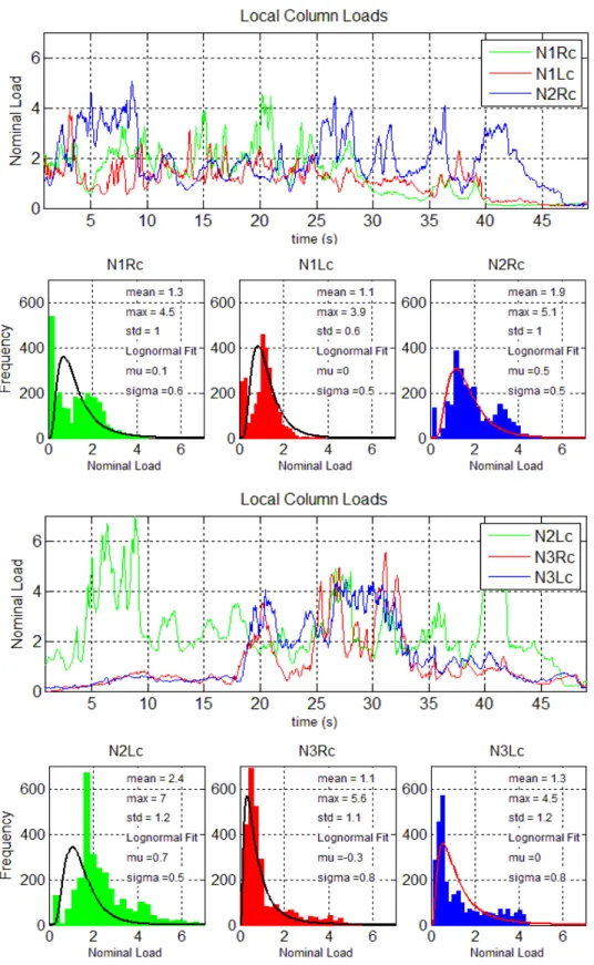
calibration factors (mean = 23.7, std = 8.4, COV = 0.35) ... 3-21 Figure 4-1: Pressure Averaging for Crushing Failure Model ... 4-3 Figure 4-2 Histograms of nominal loads of columns for the North face during event
01 ... 4-4 Figure 4-3 Histograms of nominal loads of columns for the North face during event
23 ... 4-5 Figure 4-4 Histograms of nominal loads of columns for the North face during event
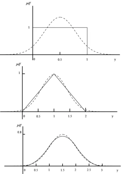
58 ... 4-6 Figure 4-5 Addition of uniformly distributed random quantities; dotted line is normal
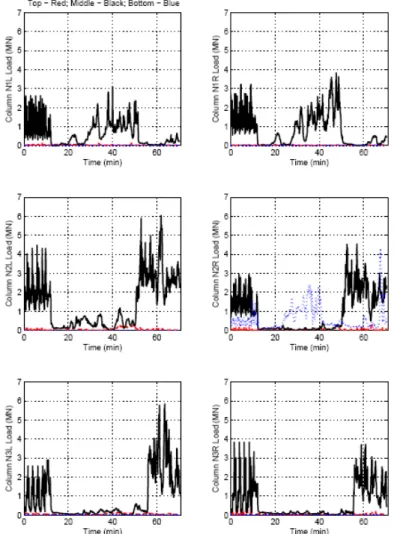
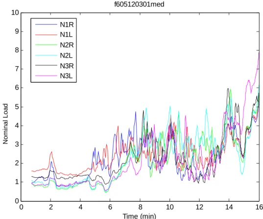
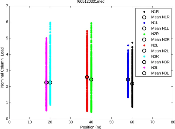
distribution (Jordaan, 2005)... 4-7 Figure 4-6: Illustration of exponential correlation function ... 4-9 Figure 4-7: Examples of correlation coefficients as a function of separation for a) crushing and b) creep... 4-17 Figure 4-8: Bi-functional correlation models chosen for a) crushing type events and b) creep type events... 4-18 Figure 4-9: “Nominal” Contact Area for Columns given Uniform Thick Ice... 4-19 Figure 4-10: Illustration of effect of bottom areas with no panels ... 4-20 Figure 4-11: Example Crushing Event ... 4-23 Figure 4-12: Example Creep Event ... 4-23 Figure 4-13: Example Flexure Event... 4-24 Figure 4-14: Variation in Contact Thickness... 4-24 Figure 4-15: Variation in Contact Width... 4-24 Figure 5-1 Rubble map showing floe impact occurring on May 12, 1986... 5-3 Figure 5-2 Loadings on North, North East and East Medof panels... 5-3 Figure 5-3 Nominal Medof column loads acting on the North face... 5-4 Figure 5-4: Distribution of Nominal Medof ice loading on the North face of the
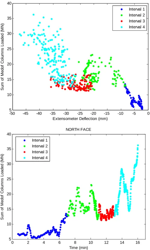
structure ... 5-5 Figure 5-5: Loading on top, middle and bottom panels in column N2R. ... 5-5 Figure 5-6: Colours represent selected intervals of interest within the data... 5-6
Figure 5-8: (a) North-South distortion, corrected for initial extensometer offsets and. ..
... 5-10 Figure 5-9 (a) North-South distortion, adjusted such that 12 minute segment with low
loading is removed. (b) corresponding load trace required to stop the floe in 15 minutes (as opposed to 27 minutes). ... 5-11 Figure 5-10: Extensometer face load versus a factored Medof face load which has undergone probabilistic averaging... 5-12 Figure 5-11: Strain gauge data has been calibrated to Medof panel group loads. Medof panel loads have been factored based on the discrepancy between them and the
extensometer values... 5-13 Figure 5-12: Application of matrix method to May 12, 1986 event... 5-15 Figure 5-13 Nominal Medof column loads acting on the North, North East and East
faces ... 5-17 Figure 5-14 Nominal Medof column loads acting on the North face of the Molikpaq
structure ... 5-17 Figure 5-15: Distribution of Medof column nominal ice loading on the face of the
structure ... 5-18 Figure 5-16: Loading on top, middle and bottom panels in column N2R. ... 5-18 Figure 5-17: The colors represent selected intervals of interest within the data. ... 5-19 Figure 5-18: Extensometer face load versus a factored Medof face load which has undergone probabilistic averaging... 5-20 Figure 5-19: Strain gauge data has been calibrated to Medof panel group loads. Medof panel loads have been factored based on the discrepancy between them and the
extensometer values... 5-21 Figure 5-20 Nominal Medof column loads acting on North, North East and East faces .
... 5-24 Figure 5-21 Nominal Medof column loads acting on the North face of the structure...
... 5-24 Figure 5-22: Distribution of Medof nominal column ice loading on the face of the
structure ... 5-25 Figure 5-23: Loading on top, middle and bottom panels in column N2R. ... 5-25 Figure 5-24: The colours represent selected intervals of interest within the data. ... 5-26 Figure 5-25: Extensometer face load versus a factored Medof face load which has undergone probabilistic averaging... 5-27 Figure 5-26: Strain gauge data has been calibrated to Medof panel group loads. Medof panel loads have been factored based on the discrepancy between them and the
extensometer values... 5-28 Figure 5-27: Comparison of ring distortion, Medof load and SG09 strain as a function of time and orientation... 5-30 Figure 5-28 Ring distortion and corresponding extensometer readings... 5-31 Figure 5-29 Sum of Panel Loads for Different Medof Groups on the North Face.... 5-32 Figure 5-30 Sum of Panel Loads for Different Medof Groups on the East Face ... 5-33 Figure 5-31 Sum of Panel Loads for Medof Group on the North-East Face... 5-33 Figure 5-32 Sum of Loads on Top, Middle and Bottom Rows of Panels on Different
Figure 5-34 Face Loads Inferred from Ring Distortions Using Matrix Method ... 5-36 Figure 5-35 Loads on Different North Face Columns versus North-South Ring
Distortion ... 5-38 Figure 5-36 Loads on Different North Face Columns versus North-South Ring
Distortion (Combined in one Plot)... 5-39 Figure 5-37 Medof Column Loads versus North-South Distortion for Unloading Part of First Cycle (only unloading part available) ... 5-39 Figure 5-38 Medof Column Loads versus North-South Distortion for Loading Part of Second Cycle ... 5-40 Figure 5-39 Medof Column Loads versus North-South Distortion for Unloading Part of Second Cycle ... 5-40 Figure 5-40 Medof Column Loads versus North-South Distortion for Loading Part of Third Cycle ... 5-41 Figure 5-41 Medof Column Loads versus North-South Distortion for Unloading Part of Third Cycle ... 5-41 Figure 5-42 Medof Column Loads versus North-South Distortion for Loading Part of Fourth Cycle ... 5-42 Figure 5-43 Medof Column Loads versus North-South Distortion for Unloading Part of Fourth Cycle ... 5-42 Figure 5-44 Medof Column Loads versus North-South Distortion for Loading Part of Fifth Cycle ... 5-43 Figure 5-45 Medof Column Loads versus North-South Distortion for Unloading Part of Fifth Cycle ... 5-43 Figure 5-46 Medof Column Loads versus North-South Distortion for Loading Part of Sixth Cycle ... 5-44 Figure 5-47 Medof Column Loads versus North-South Distortion for Unloading Part of Sixth Cycle ... 5-44 Figure 5-48 Medof Column Loads versus North-South Distortion for Loading Part of Seventh Cycle ... 5-45 Figure 5-49 Medof Column Loads versus North-South Distortion for Unloading Part of Seventh Cycle ... 5-45 Figure 5-50 Medof Column Loads versus North-South Distortion for Loading Part of Eigth Cycle (only loading part available) ... 5-46 Figure 5-51 Medof Column Loads versus North-South Distortion – Loading and Unloading During Cycle Two... 5-46 Figure 5-52 Medof Column Loads versus North-South Distortion – Loading and Unloading During Cycle Three... 5-47 Figure 5-53 Medof Column Loads versus North-South Distortion – Loading and Unloading During Cycle Four ... 5-47 Figure 5-54 Medof Column Loads versus North-South Distortion – Loading and Unloading During Cycle Five... 5-48 Figure 5-55 Medof Column Loads versus North-South Distortion – Loading and Unloading During Cycle Six... 5-48 Figure 5-56 Medof Column Loads versus North-South Distortion – Loading and
Figure 5-57 Strain Gauge 1 versus North-South Distortion – Loading and Unloading during Cycle Two ... 5-49 Figure 5-58 Strain Gauge 1 versus North-South Distortion – Loading and Unloading during Cycle Three ... 5-50 Figure 5-59 Strain Gauge 1 versus North-South Distortion – Loading and Unloading during Cycle Four ... 5-50 Figure 5-60 Strain Gauge 1 versus North-South Distortion – Loading and Unloading during Cycle Five... 5-51 Figure 5-61 Strain Gauge 1 versus North-South Distortion – Loading and Unloading during Cycle Six ... 5-51 Figure 5-62 Strain Gauge 1 versus North-South Distortion – Loading and Unloading during Cycle Seven... 5-52 Figure 5-63 Nominal Medof column loads acting on the North, North East and East
faces ... 5-54 Figure 5-64 Nominal Medof column load acting on the North face of the Molikpaq
structure ... 5-54 Figure 5-65: Distribution of Medof nominal column ice loading on the face of the
structure ... 5-55 Figure 5-66: Loading on top, middle and bottom panels in column N2R. ... 5-55 Figure 5-67: Extensometer face load versus a factored Medof face load which has undergone probabilistic averaging... 5-56 Figure 5-68 Illustration showing the effect of low panel coverage in the loaded area.. 5-57 Figure 5-69: Application of matrix method to March 7th, 1986 event... 5-58 Figure 5-70 Nominal Medof column loads acting on the North, North East and East faces of the Molikpaq structure... 5-60 Figure 5-71 Nominal Medof column loads acting on the North face of the Molikpaq
structure ... 5-60 Figure 5-72: Distribution of nominal Medof column ice loading on the face of the
structure ... 5-61 Figure 5-73: Loading on top, middle and bottom panels in column N2R. ... 5-61 Figure 5-74: Extensometer face load versus a factored Medof face load which has undergone probabilistic averaging... 5-62 Figure 5-75: Application of matrix method to March 7th, 1986 event. No zeroing of
data. ... 5-63 Figure 5-76: Application of matrix method to March 7th, 1986 event. Adjusted stiffness
matrix. ... 5-64 Figure 6-1 Measured ice failure pressure versus contact area for a wide range of
interaction and loading situations for various ice types, temperatures and strain rates (from Blanchet, 1990. After Sanderson, 1988)... 6-1 Figure 6-2 Illustration of (a) pressure-area effect; (b) increasing area for constant width panel with increasing thickness. ... 6-2 Figure 6-3 Illustration of pressure-thickness effect based on pressure data for
individual events with (a) uncorrected Molikpaq data; (b) corrected Molikpaq data... 6-3 Figure 6-4 Medof panel array numbering (letters represent columns). ... 6-4
Figure 6-5 Illustration of selected columns of Medof panel data (dark panels represent broken panels) used for: (a) thin ice events; (b) thick ice events; (c) ridge/rubble events. ..
... 6-5 Figure 6-6 Plots showing a sample Molikpaq event with: (a) linked untrimmed data,
and (b) linked trimmed data... 6-7 Figure 6-7 Data for a sample STRICE event: (a) untrimmed data, and (b) a trimmed event (after Kärnä and Yan, 2006)... 6-8 Figure 6-8 (a) Norstromsgrund lighthouse; (b) lighthouse location (Kärnä and Yan,
2006). ... 6-10 Figure 6-9 STRICE measurement panels: (a) schematic of panel numbering and
orientation; (b) mounting configuration (Kärnä and Yan, 2006)... 6-11 Figure 6-10 Indentation instrumentation and structure (a) elevation view; (b) plan view (Sodhi et al., 1998)... 6-12 Figure 6-11 Segmented indenter used in MSFIT program (Sodhi et al., 1998) ... 6-12 Figure 6-12 Case 1 (Molikpaq softening correction off; STRICE level ice filter on, duration filter off; JOIA unfiltered; Cook Inlet level ice filter on; unweighted mean) data and curve fits for: (a) mean pressure results; (b) standard deviation of pressure results...
... 6-19 Figure 6-13 Case 2 (Molikpaq softening correction on; STRICE level ice filter on,
duration filter off; JOIA unfiltered; Cook Inlet level ice filter on; unweighted mean) data and curve fits for: (a) mean pressure results; (b) standard deviation of pressure results...
... 6-20 Figure 6-14 Case 3 (Molikpaq softening correction off; STRICE level ice filter on,
duration filter off; JOIA unfiltered; Cook Inlet data excluded; weighted mean) data and curve fits for: (a) mean pressure results; (b) standard deviation of pressure results... 6-21 Figure 6-15 Case 4 (Molikpaq softening correction on; STRICE level ice filter on, duration filter off; JOIA unfiltered; Cook Inlet excluded; weighted mean) data and curve fits for: (a) mean pressure results; (b) standard deviation of pressure results. ... 6-22 Figure 6-16 Case 5 (Molikpaq softening correction on; STRICE level ice filter on, duration filter on; JOIA unfiltered; Cook Inlet level ice filter on; unweighted mean) data and curve fits for: (a) mean pressure results; (b) standard deviation of pressure results...
... 6-23 Figure 6-17 Case 6 (Molikpaq softening correction on; STRICE level ice filter on,
duration filter on; JOIA unfiltered; Cook Inlet data excluded; weighted mean) data and curve fits for: (a) mean pressure results; (b) standard deviation of pressure results... 6-24 Figure 6-18 Case 7 (Molikpaq softening correction on; STRICE level ice filter off, duration filter off; JOIA unfiltered; Cook Inlet data level ice filter off; unweighted mean) data and curve fits for: (a) mean pressure results; (b) standard deviation of pressure
results. ... 6-25 Figure 6-19 Case 8 (Molikpaq softening correction on; STRICE level ice filter on,
duration filter on; JOIA unfiltered; Cook Inlet data excluded; unweighted mean) data and curve fits for: (a) mean pressure results; (b) standard deviation of pressure results... 6-26 Figure 6-20 Case 9 (Molikpaq softening correction off; STRICE level ice filter on, duration filter on; JOIA excluded; Cook Inlet data excluded; unweighted mean) data and
Figure 6-21 Case 10 (Molikpaq softening correction on; STRICE level ice filter on, duration filter on; JOIA excluded; Cook Inlet data excluded; unweighted mean) data and curve fits for: (a) mean pressure results; (b) standard deviation of pressure results... 6-28 Figure 6-22 Case 11 (Molikpaq softening correction off; STRICE level ice filter on, duration filter on; JOIA excluded; Cook Inlet data excluded; weighted mean) data and curve fits for: (a) mean pressure results; (b) standard deviation of pressure results... 6-29 Figure 6-23 Case 12 (Molikpaq softening correction on; STRICE level ice filter on, duration filter on; JOIA excluded; Cook Inlet data excluded; weighted mean) data and curve fits for: (a) mean pressure results; (b) standard deviation of pressure results... 6-30 Figure 6-24 STRICE data (level ice filter on, duration filter on) and Molikpaq data (softening correction off) with power law trendlines. ... 6-33
1 BACKGROUND AND MOTIVATION 1.1 The Molikpaq Structure
The Molikpaq structure is illustrated in Figure 1-1, Figure 1-2 and Figure 1-3. In brief outline, the structure consists of a steel annulus, octagonal in form, serving as a caisson to support drilling operations. The structure consists of inner and outer steel plate structure connected by bulkheads. The structure rests upon a sand berm, and the core is filled with hydraulically pumped sand, uncompacted in the case of the Amauligak I65 location. The box girder deck rests upon the steel annulus, with rubber bearings between the deck and the main structure. The Molikpaq structure was placed at the Amauligak I65 location during 1986.
Details of the instrumentation are shown in Figure 1-2 and Figure 1-3 (Jefferies and Wright, 1988). Because the structure was heavily instrumented, it has served as a valuable source of information for determining design pressures for ice loading. This is the main focus of the present report, in which loads on the Molikpaq exerted by multiyear ice during the 1986 year of deployment at Amauligak I-65 are analyzed.
Many analyses in the past have relied upon the Medof panels as the primary
load-measuring device. Load estimates higher than 500 MN during key events such as that on April 12, 1986, have been suggested (Jefferies and Wright, 1988). An opposing point of view has been taken by other writers, notably by Hewitt (1994; also see Hewitt’s 2009 report in the present project and Appendix IJA - D to the present report). Hewitt estimated the maximum load at about 200 MN or less, for the event just noted.
Figure 1-2 Illustration of the Molikpaq and instrumentation (from Jefferies and Wright, 1988); for section AA details see Figure 1-3
1.2 Use of Ice pressures in Design
The study of ice pressures resulting from multiyear ice acting against structures with a vertical face is important for the design of future offshore structures for arctic areas. Figure 1-4 shows a typical framework of an analysis procedure aimed at probabilistic estimates of design loads. The key, and very important parameter concerned with force, to be studied in this report, is highlighted. Appendix IJA - A summarizes values that are suitable for probabilistic load simulations. This information needs to be updated as a result of the present study.
The Molikpaq data form the basis of many design equations, and of analyses such as that in Figure 1-4 and it is of great importance to resolve the questions raised regarding the level of loads during key events. This is the subject of the present report.
Figure 1-4: Example framework for probabilistic model. Highlighted parameter assisted by modeling of present study
1.3 Fundamental Questions and Approach
Many results have in the past been premised on the basis that the Medof panels are strictly correct. The analysis in this report shows this to be a questionable assumption as a result of possible softening of the panels. Data gathered using other instruments may form a better basis of load estimation. The following hypotheses have been proposed for consideration.
1. The Medof panels form the basis of load estimation, with other devices calibrated to them.
3. The strain gauges form the basis of load estimation, with other devices calibrated to them.
4. A best estimate compromise between the three estimates form the basis of load estimation.
The fundamental question is then: given the information at hand, under which hypothesis is the data more likely to be true? A Bayesian approach would suggest that
(
H|I)
Pr(
I |H) ( )
Pr HPr ∝ •
Equation 1-1
where H is the hypotheses, I denotes the given information, Pr
(
H |I)
denotes the likelihood of H given I, Pr(
I |H)
denotes the likelihood of I given H, and( )
HPr denotes the likelihood of H prior to receiving the information I.
This means that, for a set of equally likely hypotheses (prior to receiving information I ) (or reasonably equivalent ones), the important factor in comparing the relative likelihood of a hypothesis is the likelihood of the measurements and data which constitute I under the hypothesis under consideration, as compared to the likelihood for other hypotheses. The data are the whole body of evidence: Medof panel readings, extensometer readings, strain gauge readings as well as all the other information such as observations of the state of the sand core, inclinometer readings and so on.
There are ample reasons to reject Hypothesis (3), since there is great uncertainty in these measurements. Certainly based on the analysis in the present report, (1) is questionable. This would involve rejecting the extensometer readings and accepting the Medof calibration, while there are good grounds to question the accuracy of the Medof panels. With regard to (4), the weight of evidence favours (2). The Medof panel results contain excellent information, but a refined calibration constant is needed. For the present report, this is based on the extensometer results.
1.4 Velocity Effects
In interpreting the data, the mechanics of failure varies with the speed of interaction. This will have a strong influence on the distribution of load. Figure 1-5 shows the effect of velocity in medium scale indentation tests. Slow interactions result in “ductile” or “creep” failure (this is not pure creep but damage-enhanced creep illustrated in the left hand side of Figure 1-5). This kind of interaction will result in pressures that are more evenly spread out than those involving brittle fracture (illustrated in the right hand side of Figure 1-5). Much higher gradients of pressure will exist if brittle fracture takes place than in the ductile failures, and this is important in interpreting data and in future modelling.
Figure 1-5: Medium scale insitu testing with interaction area of 1.0 m2: Left, 0.3 mm s─1, ductile
failure; right, 10 mm s─1, brittle failure. Courtesy Dan Masterson
1.5 Definition of an Event: Data Files
A further factor that should be borne in mind is the definition of an event. In the earlier work (Jordaan et al., 2006), an event was a major ice-structure interaction, and the data from the Molikpaq and other measurements (e.g. STRICE) result in events of different durations. Various modes of failure were included. Figure 1-7 is an example. In the present project, the events have been divided further into sub-events, in collaboration with Brian Wright, as shown for the event of Figure 1-7 in Figure 1-8 and Table 1-1. This was extended to a set of events. These are denoted BDW data. This does represent a step forward in understanding as the different sub-events correspond to different failure modes of crushing (CR), creep (SLW), mixed mode (MM) and sliding (SLD).
Some comments need to be made. First, if the time intervals are too short, the statistics for the events are also short and will not be representative of an event of adequate duration for this purpose. The Medof panel is based on the localized areas (about 10% say), and are not necessarily representative of the whole face, and are then difficult to use in calibration or in modeling if this inadequacy is compounded by shortness of the event durations. (Here, the extensometer-deduced loads might assist.) Second, for future modeling of the kind in Figure 1-4 there are often in reality some mixed-mode aspects of the crushing failure process, and one might want to build the model on a more robust methodology that captures the essential points.
To enlarge on the point just made, an event could well include some periods of mixed-mode behaviour, and still be considered stationary. Figure 1-6 shows how such an event could be composed. Practical idealizations will doubtless included some periods of mixed-mode failure. It is also noted that averaging is appropriate even for non-stationary events. In practical modelling, it is convenient to divide the loading scenarios into series of stationary events. Too much can be made of the existence on non-stationary periods as
Time
Pure Crushing Failure
Mixed Modal Failure
Event Duration
Figure 1-6: Illustration of potential composition of an ice loading event The files available for use are the following.
1. Dynamac files
2. Trimmed event files (inhouse) corrected for panels not working
3. Trimmed event files (Taylor, 2009) for comparison with STRICE and other data (Chapter 6)
4. BDW subevents—events compiled by Brian Wright 5. CHC subevents.
In the present study, the BDW events were used to estimate the correlation constants for averaging (included in the present report, Chapter 4). In the June 2008 report they were used also to calibrate the extensometer readings to the Medof panel readings, not a good procedure given the uncertainty surrounding the Medof panel calibration. The shortness of the durations makes the BDW files difficult to use effectively for calibration. The Dynamac and inhouse trimmed files were used for evaluation of events and for calibration in the present report.
Figure 1-7: Original characterization of event based on Medof panel readings (Jordaan et al., 2005) T o tal N o m ina l lo ad on Pa nel s T o tal N o m ina l lo ad on Pa nel s
Figure 1-8: Event of Figure 1-6 with sub-events of the present study, indicated by vertical red lines
1.6 Geotechnical Aspects and Klohn Crippen Berger (2009)
Appendix IJA - C contains a review by C-CORE of geotechnical work done in the past on the Molikpaq response, principally focused on the April 12 events together with an addendum on the geotechnical response of the sand core. This review does not deal with the state of the sand in the core of the Molikpaq. To put this into focus, Appendix IJA - D by Kevin Hewitt has been added, in which the state of the sand core is discussed. Subsequent to the ice loading events of 1986, a Joint Industry Project was carried out to study the events and associated measurements of the Molikpaq. This is referred to as the “1986 JIP”. The recent report by Klohn Crippen Berger (2009) provides a summary of this JIP. The measurements on the Molikpaq together with the 1986 JIP and its original set of reports have in fact formed the basis of the present study. The IJA project team has concluded that the results of the 1986 JIP need reconsideration. The key aspect that should be reconsidered is the strong reliance on the original calibrations of the Medof panel in the 1986 JIP. The team is consequently in disagreement with the Klohn Crippen Berger interpretation, which is closely aligned with the 1986 JIP reports. It is considered that the arguments in the report supporting the original Medof calibration are not well-founded. It is accepted generally that hydraulically placed sand pumped through a pipeline is loose and not dilative (see Hewitt, 2009), and furthermore, prone to
liquefaction. There are uncertainties in the Sandwell results, acknowledged by the present team, but these are outweighed by the far greater uncertainties in the Medof panel results. In fact, the points raised by Klohn Crippen Berger have been dealt with in our work. The ice mechanics in the report omits reference to work after the 1986 JIP in which the behaviour and failure of high-pressure zones has been discovered. The ice mechanics, as a result, are out of date. No cause to change the present approach has been found in the Klohn Crippen Berger report.
While there are disagreements as to the precise state of the sand core, the estimates based on a loose fill agree in essentials with our current estimates of load. In general terms: our advice from Ryan Phillips is that the three significant load events (March 7/8, April 12, and May 12) exceeded the “basal shear resistance” (say 140-180 MN), “but not by very much” (C-CORE Technical Memorandum, July 14, 2009). The state of the core would also be affected by the dynamic shaking during these events. Our current best estimates of load for these events based on the extensometer readings are somewhat less than 200 MN except for the April 12 event which is somewhat greater. The decelerating floe analysis suggests that the load in the May 12 event is less than 140 MN. But the
geotechnical estimates are beginning to fall into the same “ballpark” as other estimates.
1.7 Face Load versus Global Loads; Pressures
Figure 1-9 shows face loading and possible global loading in idealizations. In some studies, a constant factor has been used to convert from face to global loading. The situation in reality is more complicated than this; Figure 1-10 show patterns observed in the Dynamac report (north is being used here as an arbitrary reference direction). Figure
N
N NN
Figure 1-9 Loading scenarios; face loading (left) and global load (right)
(a) (b) (c) (d) (e) (f) (g) (h) (i) (j) (k) (l) (a) (b) (c) (d) (e) (f) (g) (h) (i) (j) (k) (l)
(g, h, i, l) (e, f, j) (b, d, e, f, j)
(Partial loading sub event) (Partial loading sub event)
(g, h, i, l) (e, f, j) (b, d, e, f, j)
(Partial loading sub event) (Partial loading sub event)
Figure 1-11 Some idealizations of the loadings in Figure 1-10; text under each idealization refers approximately to cases in Figure 1-10.
Figure 1-12 shows patterns that have been used in analysis; the face and the uniformly distributed load (udl) in our matrix method (Section 2.5) and in Sandwell (1991). The latter reference also included a “most likely” scenario with reduced loads on the corners (top right in Figure 1-12). The corner load (bottom left) was also used in the matrix method developed in the present report.
A key message is that the pattern considered should correspond as closely as possible to the observed situation in the event under consideration, with the constants for
N N NN N N N N
Figure 1-12 Loading patterns used in analyses; face load (top left), uniformly distributed load (top centre), “most likely” distributed load (top right), used in Sandwell (1991), and corner load (bottom left)
1.8 Organization of the Present Study
In the report, Chapter 2 includes a description of the Molikpaq structure and its response to load. This includes discussion of the Sandwell (1991) report, and the matrix method developed by the present group to account for loading on multiple faces. Chapter 3 includes a discussion of the principal load measuring devices: the extensometers, the Medof panels and the strain gauges. In Chapter 4, the technique of probabilistic averaging is discussed, with results on correlation and a comparison of linear and probabilistic averaging. Nine full events and their subevents were analyzed and these results were presented at the June 2008 project meeting in Calgary. These results are discussed briefly in Chapter 5 and given in more detail in Appendix IJA - B. The loads deduced from the Medof panels have been termed “nominal” loads because of their uncertainty. Detailed analysis of certain events is given in Chapter 5. A comparison with other data sets is given in Chapter 6 (STRICE in particular), with conclusions of the study in Chapter 7.
2 THE STRUCTURAL BEHAVIOUR OF THE MOLIKPAQ 2.1 Deformations of the Structure
Extensometers have been used to measure deformations of the main structure. The box girder deck rests upon rubber bearings which in turn rest upon the steel annulus (the main structure) (Figure 2-1). The extensometers measure the deformation between the box girder deck and this structure. The Molikpaq acts essentially as an elastic “proving ring”. The use of calibrations from finite element analyses is a good way to obtain stiffnesses for global load estimates. The difficulty lies in obtaining a clear assessment of the boundary conditions imposed by the foundation and in obtaining the appropriate finite element analysis to obtain the stiffness.
Box girder deck
Extensometer
Rubber bearing
Figure 2-1 Box girder deck resting on main structure
2.2 Boundary Conditions
In calibrating the extensometers and the strain gauges, it is most important that the deformation of the caisson be determined as well as possible. Figure 2-2 shows
schematically a free-body-diagram of the caisson. The division of load between the base and the core is most important. The figure is intended as a guide (schematic); we know that there is active pressure at the rear and sides. The main point to be determined here is the division between the base friction and the core. Ryan Phillips has kindly provided Figure 2-3. This suggests that the base friction is mobilized before the core resistance. Estimates of the base resistance (caisson friction) are in the range 140 to 180 MN based on the loaded weight of 380 MN (Sandwell, 1991) and a coefficient of friction of 0.364 to 0.466 (friction angle of 20º to 25º) (note that weathered steel on medium dense sand is under consideration; Hewitt, 2009). Up to the value of frictional resistance, there will be some deformation of the caisson, leading to core resistance, say 10%. Above this load, transfer of force to core will increase.
Figure 2-2: Schematic illustration of the boundary conditions imposed on the Molikpaq by the foundation. The sand core will have active resistance on the face opposite to the loaded face above.
Figure 2-3: Transfer of load from the caisson to the foundation (provided by Ryan Phillips). Numbers opposite springs indicate the displacement in mm required to activate the corresponding resistance.
2.3 Finite Element Analyses
Many of the finite element studies have concentrated on soil behaviour (Jeyatharan, Sladen (EBA), Altaee and Fellenius – See Appendices IJA - C and IJA - D). In these assumptions of a rigid structure are made. The deformations given in the results are of the foundation response and are irrelevant to the structure stiffness, except in the very
important sense of obtaining the correct boundary conditions in Figure 2-2. But generally, assumptions of dense sand have been made. In terms of proper structural analysis that can be used for calibration of extensometers, the report by Klohn Crippen Berger (2009) is no improvement on the other geotechnically oriented papers.
The references noted can not be used for extensometer calibration. A study that does address the ring distortion needed for calibrating the extensometer is the Sandwell (1991) report, “Extensometer Calibration for Ice Load Measurement”, which was also calibrated back to the original Stardyne analysis.
2.4 Sandwell (1991) Report
The report was written as part of the 1986 JIP for Gulf Canada, and represents an analysis of the structural response, and as noted, was compared to the original Stardyne analysis, with good agreement. At the same time, reservations are expressed regarding the input assumptions. As in the report, we shall consider loading in the North-South direction as a reference for discussion. The results are expressed as “Ring Distortions” in mm and “Load Distortion Ratios” in MN mm─1, which represent the calibration factors of the extensometers.
The stiffness values vary considerably (Sandwell, 1991) depending on whether one considers the loading on the centre face (i.e. the central northern face, about 58 m long) or the entire side, which was modelled as a N-S uniformly distributed loading (udl) of the two (NE and NW) corner faces of the octagon as well as the centre face. See Section 1.7 for a discussion of loading patterns. In summary, Sandwell (1991) considered the
following:
1. uniformly distributed load (udl) over the centre face only, 2. uniformly distributed load (udl) over the entire width, and 3. the “most likely” load distribution;
see Figure 1-12.
Loading case 2 above included the same north-south distributed loading on the two corner faces as well as on the centre face. Since these loadings were in the north-south direction, other loads were applied to achieve equilibrium. These consisted of a frictional force on the side of the caisson and a lateral force; see Figure 2-4 and Sandwell (1991) for details.
µNc Nc
Lc
HBS
Hc Hc HICE (Horizontal Ice Force)
45o HICE µNc Nc Lc µNc Nc Lc HBS
Hc Hc HICE (Horizontal Ice Force)
45o
µNc Nc
Lc
HBS
Hc Hc HICE (Horizontal Ice Force)
45o HICE µNc Nc Lc HICE µNc Nc Lc
Figure 2-4 Loading assumption used by Sandwell (1991) for udl over whole width
In reality one might expect some attenuation of the udl towards the edges, and on the corner faces. The “most likely” load used by Sandwell consisted of a udl over the centre front north caisson, and a triangular load on the NW and NE sides decreasing from the
udl value on the centre face to zero at the outside corners. This seems to be a reasonable
practical interpretation of the load over a face and nearby corners. At the same time some concern is expressed that the lateral load applied at the corners might be too high,
dictated by the fact that the applied loading is in the N-S direction.
In addition, the inclusion of the lateral force Lc would tend to make the structure stiffer than it is in reality. As a result, the load distortion ratios for global load would tend to be too high and exaggerate the global loads.
General Conclusions of Report
Some general conclusions from the report are as follows:
1. The stiffness (Load Distortion Ratio) was found to be in the range 2.0 to 4.2 MN mm─1.
2. The interplay between loads on the 45° sides and the face are important and should be taken into account where necessary in calibration and load estimation. Since the stiffness values quoted are about half of the prior estimates based on the Medof panels (6 MN mm─1), it was surmised in the report that the results indicate that either “the actual structure and soil interaction is much stiffer than the model, or that the application of the ice load is lower or that base shear is more significant than assumed...”
Assumptions Regarding Share of Base Shear
One important assumption was that the share of the resistance offered by base friction was fixed. This was generally set at 40% although some sensitivity runs were carried out. As discussed above, it is considered that too much load is being transmitted into the core; about 80-90% might be transmitted through base friction.