RESEARCH OUTPUTS / RÉSULTATS DE RECHERCHE
Author(s) - Auteur(s) :
Publication date - Date de publication :
Permanent link - Permalien :
Rights / License - Licence de droit d’auteur :
Institutional Repository - Research Portal
Dépôt Institutionnel - Portail de la Recherche
researchportal.unamur.be
University of Namur
From average travel time budgets to daily travel time distributions
Hubert, Jena-Paul; Toint, Philippe Published in:
Transportation Research Record
Publication date:
2006
Document Version
Early version, also known as pre-print
Link to publication
Citation for pulished version (HARVARD):
Hubert, J-P & Toint, P 2006, From average travel time budgets to daily travel time distributions: Appraisal of two conjectures by Kölbl and Helbing and some consequences. in Transportation Research Record. pp. 135-143.
General rights
Copyright and moral rights for the publications made accessible in the public portal are retained by the authors and/or other copyright owners and it is a condition of accessing publications that users recognise and abide by the legal requirements associated with these rights. • Users may download and print one copy of any publication from the public portal for the purpose of private study or research. • You may not further distribute the material or use it for any profit-making activity or commercial gain
• You may freely distribute the URL identifying the publication in the public portal ?
Take down policy
If you believe that this document breaches copyright please contact us providing details, and we will remove access to the work immediately and investigate your claim.
From average travel time budgets to daily travel time distributions: an appraisal of
two conjectures by Kölbl and Helbing and some consequences
Submitted July 31, 2005 Jean-Paul HUBERT* Philippe L. TOINT
Transportation Research Group The University of Namur Rue de Bruxelles 61 B-5000 NAMUR BELGIQUE Tel (32) 81 72 49 18 Fax (32) 81 72 49 14 [email protected] [email protected] * From Sept. 1, 2005: INSEE
Département des prix à la consommation, des ressources et des conditions de vie des ménages 18, Boulevard Adolphe Pinard
F-75675 PARIS Cedex 14 FRANCE
4999 words, 5 figures, 5 tables = 7499
Abstract
An analysis of three travel surveys (in Belgium, France, and Great Britain,) is used to investigate two conjectures by Kölbl and Helbing (2003). The first one suggests a relation between mode choice and human energy expenditure for travel, which is assumed to be constant in time and space. The second one is the assumption that the distribution form of daily travel time can be derived from an entropy maximization model. The analysis shows the link with energy expenditure to be questionable, but also provides alternative views of travel time analysis. In particular, the distribution of daily travel time is shown to be well approximated by three different models. Weekly travel time expenditure are also shown to present different
characteristics than the more commonly used daily ones, reinforcing the argument for inclusion of weekly regularities in travel behaviour analysis and modelling.
1) Introduction
Travel is commonly regarded as a derived activity determined by the place and utility of other activities which are combined in a daily activity chain. The activity chain is supposedly designed to maximize a daily utility by aggregating activities located in more or less remote places, some of them being compulsory (see for instance Bhat and Koppelman 1993). The total daily travel time may thus appear as a dependent phenomenon but it is also a limiting factor for the activity chain seen as an aggregating process of utilities (Dijst and Vidakovic 1997; Cornélis et al. 2004b). It is thus an important piece of information in many activity-based travel demand models.
It is well known that the average daily travel time at a regional level varies little over time and space, as pointed out first by Zahavi (1977), even if disaggregated travel times differ from one social group to another and can reveal discrepancies within social behaviours. Many studies have analyzed the aggregated average travel time and its (slow) evolution, as a tool to investigate travel behaviour (see the review by Mokhtarian and Chen 2004). While this indicator is clearly on the rise in the USA, it is much more stable in Western Europe, almost unchanged in Great Britain between 1972 and 2000, or in France between 1982 and 1994, or slightly increasing in the Netherlands (see for instance Pendyala and Bhat 2004; Joly 2004; Madre and Maffre 1997; Quetelard 1998; Van Wee at al 2002; DETR 2005). These evolutions raise new behavioural questions, including the possibility that travel time might become less of a disutility than in the past, or even sometimes turn into a positive utility because of the improved comfort of cars, carriages or coaches, or because of devices, such as laptop computers or cellular phones, which provide new possibilities to use one’s travel time (Van Wee et al. 2002; Mokhtarian and Salomon 2000; Lyons and Urry 2004; Cirillo and Axhausen 2004).
When considering either the urban sprawl problem (in the light of Zahavi’s hypothesis on the proportional increase of travel speed and travel distances), or possible changes in the primary utility of trips, analysis generally emphasizes average daily travel times. Yet, it is also very important to know what kinds of trips are concerned by the evolution of behaviours, and this naturally leads to considering the complete statistical distribution of travel times. As a consequence, comparing such distributions is therefore of interest.
To our knowledge, only a small number of descriptive studies have paid attention to the empirical distribution of the daily travel time (e.g. Zeibots 2003), although some discussion on duration distributions for modelling issues can be found: simulation of individual activity chains using hazard functions to estimate the end of activities (Bhat 2000; Joly 2004) or of car
emissions. Nair and Bhat (2003), for instance, assume that car trip durations follow a log-normal distribution. A paper by Kölbl and Helbing (2003) stands out because it attempts an explanation both of the average travel time stability and of its distribution. More globally however, the debate on the stability of travel time expenditure or on its consequence, Zahavi’s hypothesis of the “rational locator” (Levinson et al. 2004), remains mainly focused on daily travel time averages, even if they are sometimes disaggregated by age, status or geographical classes of individuals. These observations all suggest that a careful analysis of daily travel time distributions could provide useful additional information for a more comprehensive comparison of the evolution of mobility behaviours between two nationwide or metropolitan travel surveys. It is the purpose of the present paper to contribute to such an analysis. In a first part, conjectures by Kölbl and
Helbing (2003) on a possible link between travel time, mode choice and human energy
expenditure by the traveller is examined using three different data sources (section 2), and this link is shown to be far from obvious (section 3). We argue however that the remarkably coherent form of the implied density functions may be helpful in comparing travel time distributions (section 4). We finally present some empirical evidence of weekly regularities in travel behaviour that are reflected in a right shift of the associated travel time distribution curves compared to the daily ones (section 5). Some conclusions and perspectives are finally discussed.
2) The Kölbl and Helbing conjectures
For daily travel time distribution to reflect true behavioural patterns, it is necessary to assume that the stability or instability of daily travel time distribution and of its average are structural, i.e. that it is controlled at the level of the society as a whole by temporal structures, which may have their origin in biology, anthropology or social conventions, and are a basis for social institutions, either traditional or emerging.
In their article, Kölbl and Helbing (2003) first conjecture that the relative stability of average travel time has its source in a biological factor, which regulates the average daily human energy expenditure for travel. They first establish that not only has the average daily travel time been stable in Great Britain for almost 30 years, but the average daily travel times of one transport mode users have been stable at significantly different levels. They estimate the mean coefficients of human energy expenditure by time of travel for each mode of transport that could, by the conversion of travel times into energy expenditure, resolve all discrepancies in the daily travel times between transport modes. After the checking from physiological tables that these
estimations are reasonable, they then conjecture that the average daily human energy expenditure for travel is a universal constant that explains the stability to the average travel time.
Such universal constant authorizes significant individual, and daily variations. Thus, they present the hypothesis that the distribution of daily energy expenditure basically follows an exponential law which maximizes its entropy for a fixed average value. But they also recognize that a (small) energy/time threshold exists, reflecting the low probability of very small amount energy or time dedicated to travel. This so-called “Simonson effect” is explained by the fact that there are fewer activities for an individual to perform at very short range.
Gathering these two views, they then suggest that daily energy expenditure follows a density function of the type: f(En)= N × exp(– a / En – En /b ) where En is a normalised daily energy
expenditure (i.e. divided by the average), and where N, a and b are distribution parameters constant through modes, space and time. Because of the first conjecture, the daily travel time distribution then has to follow a similar distribution, for which they propose the values N = 2.5, a = 0.2, and b = 0.7, on the basis of the British NTS data for the years 1972 to 2000. If correct, this conjecture is of clear interest because of its macroscopic explanatory potential, in particular regarding aggregated mode choice. It is therefore of interest to validate it.
3) Testing the hypothesis of constant energy expenditure
Our validation attempt is based on three nationwide travel surveys in Belgium (MOBEL 1999, SSTC-GRT), France (ENT - Enquête Nationale Transport - 1993-1994, INSEE-Inrets), and Great Britain (NTS 1999-2001, Stats UK), from which we extract the total travel time, for one
individual, for all transport modes in one day, including waiting time. As usual, the three data sources must be handled with care because of differences in survey methodology: the French data is not strictly comparable with the Belgian and British ones, because the survey period is
different: it excludes holidays and week-ends. Similarly, the Belgian and the British data differ by the fact that Belgian respondents are surveyed on one day only and British respondents on a whole week. Non travellers are excluded from the analysis in all three surveys because mobility rates depend very much on the survey methods (see Armoogum et al 2005). The resulting databases then contain about 5,300; 11,700; and 22,000 travellers’ days in Belgium, France and Great Britain, respectively.
We start by a brief discussion of the conjecture of constant energy expenditure for travel (elaborating from the preliminary analysis by Gobeaux 2004, and Cornélis et al. 2004b) and examine how average daily travel times are levelled for the users of different transport modes. In order to convert travel time into energy expenditure by mode, we use the coefficients proposed by Kölbl and Helbing after their study of the British data from 1972 to 1998 (given in the last column of Table 1). The analysis is made for classes of travellers whose declared trips were made only with this mode or walking, and the share of walking is country dependent. In the three surveys, travel times also include waiting times, but only in the British data are waiting times explicitely known and taken into account. At last, if the three surveys provide data on all the means of transport used in every trip, travel times are not dispatched by modes in the French survey, so that the total travel time of a trip has to be affected to the main mode. These
differences explain why the ratios of daily human energy expenditures by daily travel times for each class of travellers are not strictly equal in the three countries and slightly differ from Kölbl and Helbing’s coefficients.
According to the Kölbl and Helbing first conjecture, energy expenditures and travel times of exclusive users of a given transport mode should be almost identical. Unfortunately, this conclusion is not supported by our data, as is reported in Tables 1 and 2. If the conjecture were valid, the shorter the average daily travel time for an exclusive user of a mode, the more tiring (in the sense of larger human energy expenditure) the use of this mode. This seems to be consistent for the data, except for car passengers, for whom the energy expenditure per time unit is
surprisingly high. This would imply, in particular, that being transported by car is much more tiring then driving, a somewhat counter-intuitive conclusion. This problem was already noted by Kölbl and Helbing, who indicated, without further analysis, that car passengers might have proportionally longer access and egress walking trips.
In our opinion, the explanation for the short daily travel time for car passengers (if at all) could be more sociological than biological: car passengers are more often nonworking people, especially students or housewives without driving license, and their places of activities are generally closer to their home than work place is. Therefore, the conversion of travel time into human energy cannot, in our view, completely abolish the gap between car passengers and other travellers.
MOBEL (Belgium) ENT (France) NTS (Great Britain) Transport mode Average energy (kJ) Standard error Average energy (kJ) Standard error Average energy (kJ) Standard error Average human energy/minute of travel (kJ/min) train 803 145 744 49 566 21 4.0 car (driver) 642 14 578 8 624 3 8.2 bus 798 37 878 18 681 6 9.2 car (pass) 628 20 829 30 617 4 10.4 bicycle 780 73 773 44 769 15 14.6 walk 602 27 647 13 851 7 15.4 > 2 modes 885 24 913 13 919 6
TABLE 1: Average daily human energy expenditures for classes of travellers (conversion of travel time into energy expenditure uses Kölbl and Helbing’s coefficients, last column on the right; the coefficient for train is used for waiting time in the British trips)
Data: GRT-SSTC 1999, INSEE-Inrets 1994, Stats UK 2001.
MOBEL (Belgium) ENT (France) NTS (Great Britain) Transport mode Average travel time (min) Standard error Average travel time (min) Standard error Average travel time (min) Standard error train 105 15.2 167 8.9 116 2.7 car (driver) 73 1.5 66 0.9 76 0.3 bus 73 2.6 90 1.7 82 0.6 car (pass) 57 1.7 78 2.8 59 0.3 bicycle 53 5.1 53 3.0 55 1.1 walk 39 1.7 42 0.8 57 0.5 > 2 modes 105 2.7 103 1.7 116 0.7
TABLE 2: Average daily travel time for classes of travellers Data: GRT-SSTC 1999, INSEE-Inrets 1994, Stats UK 2001.
Two further difficulties regarding the first conjecture also arise from our analysis. The first is to explain why travellers who have used more than two modes (and were excluded from the analysis by Kölbl and Helbing, who considered only exclusive mode users) show energy
expenditures higher than expected compared with exclusive mode users, as is apparent in the last lines of Tables 1 and 2. Finally, the average expenditure of 615 kJ/day (147 kcal/day) that Kölbl and Helbing assume to be universal and constant, is a surprisingly small expenditure for an average person who already consumes 250 kJ/h just for sustaining one's metabolism (Monod and Flandrois 2003). Moreover, one could argue that the number of calories burnt for travel has a completely different meaning (in terms of physical effort) if the travel time is 30 min or 2 hours. For these three reasons, we fail to be convinced by the conjecture of constant human energy budget for travel.
4) Travel time distributions
If the energetic explanation of small variations in travel time expenditure over time remains, in our view, questionable, the fact that these variations are small (the daily travel time averages are indeed very similar in the three surveys: 75.3 minutes for Belgium, 75.5 for France and 73.5 for Britain) remains highly interesting and deserves further analysis. We may then consider the second conjecture, namely that the density function for normalized daily travel times (denoted by “Tn”) follows the proposed formula.
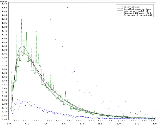
Unfortunately, the observation of times or duration is prone to a well known effect of brutal rounding to the nearest 5 or 10 minutes, for small trips, 10 or 15 minutes for longer trips (Rietveld 2005, Madre and Armoogum 1997). The frequency histogram of the travel-times therefore show very high frequencies for round figures and very low in between (in blue “+”). Before comparing it with continuous models, it therefore seems relevant to compute a smoothed histogram with sliding averages. The results presented below use a smoothing on an interval of 11 minutes (in green “×”, joined), but other value were tried that led to very similar conclusions. We next compare, in Figures 1 to 3, the empirical distributions for our three data sets, raw and smoothed, with different continuous ones:
- (1) a log-normal distribution of parameters z and s,
- (2) a reference (KH) curve: 2.5 × exp(– 0.2 / Tn – Tn / 0.7), which is that proposed by Kölbl and
Helbing (2003),
- (3) a function: N × exp(– a / Tn – En /b), where N, a and b are calibrated on the raw data with
the constraint that the density integral must be equal to 1 (N > 0, a > 0 and b > 0).
The parameter calibrations for models (1) and (3) were performed on the raw data using the LANCELOT (see Conn, Gould, Toint, 1992, and Gould, Orban and Toint, 2003) package for nonlinear optimization, and the resulting values for an average day given in Table 3. Calibration on smoothed data gives very similar results.
The two models (KH, possibly recalibrated, and log-normal) have two different interpretations. The coefficient “a” makes all the difference between the calibrated distribution and the
exponential distribution associated with the entropy maximization hypothesis. Kölbl and Helbing explain that difference by a threshold effect making very short trips quite infrequent. The
probability of a very short trip to occur is mostly determined by “a”, thus it can be said that this coefficient is an indicator of that threshold. When “a” is superior to zero, the distribution has a maximum when Tn is equal to the square root of (a × b). The coefficient “b” impacts the speed of
decrease for the density, sometimes called “distance decay” by spatial analysts (De Vries et al. 2004). On the other hand, the log-normal adjustment could signify that, since its logarithm is Gaussian, daily travel time varies around a value which is exp(z), and corresponds to 70% of the average (about 50 minutes). The probability of a daily travel time being t × exp(z) (t ≥1) is then equal to that of a daily travel time being exp(z)/t. This suggests that travel time perception could be logarithmic (as is the perception of sound), but this obviously requires a sounder behavioural analysis.
FIGURE 1: Belgian normalized travel time distribution, raw, smoothed and models (data: MOBEL, GRT-SSTC 1999)
FIGURE 2: French normalized travel time distribution, raw, smoothed and models (data: ENT, Insee-Inrets 1994)
FIGURE 3: British normalized travel time distribution, raw, smoothed and models (data: NTS, Stats UK 2001)
mean daily
travel time N a b max. of curve (3) z s
MOBEL 73.3 min 1.89 0.12 0.77 0.30 -0.38 0.91 ENT 73.5 min 2.11 0.15 0.74 0.33 -0.34 0.84
NTS 75.3 min 2.52 0.19 0.69 0.36 -0.33 0.83
TABLE 3: Coefficients for the three nation-wide daily travel time distributions
The first conclusion that can be drawn from the figures is that the smoothed frequency histogram and the three continuous (model) curves are remarkably similar. For all datasets, the log-normal peak is sharper than that of the other curves. Deciding which distribution model fits the data best is complicated. Statistical tests such as Kolmogorov-Smirnov are negative for all three models. Note that the drastic jumps occurring in the cumulative frequency at rounded durations make the context difficult.
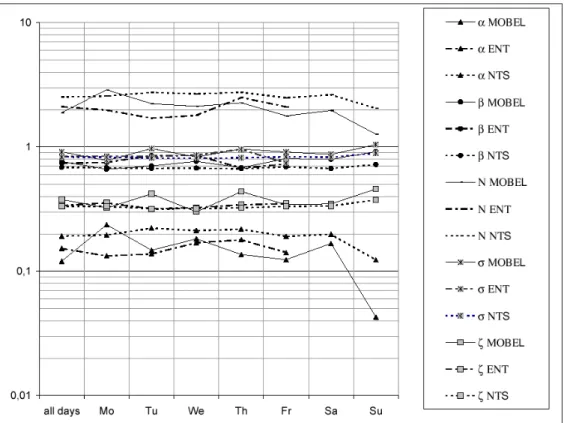
The calibration of coefficients of the curve (3) can also be performed for each day of the week separately. The resulting values are illustrated in Figure 4, where only the values for Sundays seem really apart from the others. (Remember that the French data cannot be used for week-ends). It is worth noticing that there are correlations between the coefficients. For instance, z and
s are correlated together and, negatively, to a, which indicates that further statistical analysis could be of interest.
FIGURE 4: Variations of the calibration coefficients according to the day and the country Data: GRT-SSTC 1999, INSEE-Inrets 1994, Stats UK 2001.
The second observation is that the value Tn=1, which corresponds to the average travel time,
exceeds around three times that of the frequency peak (circa 0.33). Moreover the value of the density at the peak is 25 to 35% higher than that at the average travel time. In cumulative frequency, the average corresponds to 66%. The average travel time therefore may not be as comprehensive and neutral an indicator as wished. It is known, but seldom stressed, that these distributions are significantly left skewed and that their variance is quite high. Indeed, the value of the standard deviation is generally similar to that of the average when all transport modes are mixed. The tail of the distribution is problematic. For instance, the average daily travel time decreases of 9.9%, 9.9%, and 9.6% when the 2% highest values are removed from the Belgian, French and British data, respectively. The left part is not perfect either. Rietveld (2005) points out that, the distribution being skewed and the reporting times being rounded, the probability of rounding travel time upward is higher than the probability of rounding downward. His
conclusion is that travel times are overestimated. The same thing occur if we compare daily travel time from a transport survey based on a trip diary and from a time-use survey based on an activity diary. Time-use surveys round times to 10 minutes while transport survey’s respondents round them mostly to 5 minutes, and travel times are accordingly longer according to time-use surveys than to transport surveys (Armoogum et al. 2005, Castaigne and Hubert 2005).
A better indicator is, in our view, the value of the daily travel time at the frequency peak,
although it cannot be estimated directly but only from the smoothed histogram or the continuous curves (2) and (3), in which case it is equal to the square root of a x b. The indicator could be completed by some measure of the decreasing rate, such as b for the optimised KH models.
5) Density functions on a weekly basis
The analysis presented so far is uniquely based on one-day observations, as both Belgian and French surveys are designed to catch trips on a single day (the French data includes a weekly diary but only for cars). The British survey is however conducted on a weekly basis, which makes it possible to examine the variations of individual behaviour during the week. Such
variations are an important issue in the modelling of activity and trip generation, and have lead to dedicated research on long period mobility surveys (Axhausen et al. 2002, Löchl et al. 2005). We next investigate the question of whether density functions for seven or five (excluding week-end) days average travel times differ from the density function for one day. If they remain close, this indicates a substantial replication of a specific behavioural pattern during the week. If they differ, this indicates that people have different patterns for different days of the week. The number of different daily patterns per week can then be considered as another indicator of the evolution of mobility behaviours and comparing density functions can be seem as a tool to monitor such an evolution.
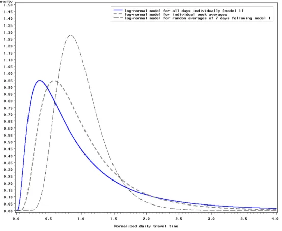
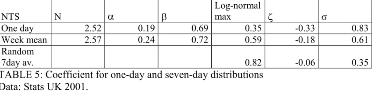
Figure 5 shows three density models for daily travel time for which we have chosen the log-normal parametrization. The first is the daily density obtained (as above) by considering an average day. The second (with its peak at the same level, but shifted to the right) is the density obtained by considering weekly travel time expenditures. The third (with its significantly higher peak, even further to the right) is that obtained by averaging 7 random variations generated by sampling from the distribution for an average day. The corresponding log-normal parameters are given in Table 5, together with calibrated KH parameters (the corresponding curves are similar and thus not shown).
NTS N a b Log-normal max z s One day 2.52 0.19 0.69 0.35 -0.33 0.83 Week mean 2.57 0.24 0.72 0.59 -0.18 0.61 Random 7day av. 0.82 -0.06 0.35
TABLE 5: Coefficient for one-day and seven-day distributions Data: Stats UK 2001.
Interestingly, the weekly travel time expenditure density is significantly different from the two other ones. This indicates the presence of behavioural regularities with weekly period: indeed, if the travel times of the seven days of the week were completely independent, the translation would be far more important and the variance smaller, as illustrated by the third curve.
This result is intuitively not overly surprising since one may anticipate that specific activities, like sport, cultural meetings or specific shopping, only occur with a weekly period. However, we find it interesting that this intuition is actually vindicated by the data. This result bear similarities with that by Löchl et al (2005), who have shown that the distribution of trips for one day
observations is very left skewed while their distribution of individual averages for 6 weeks is closer to a normal distribution around the general average.
6 Conclusion
In this paper, we have considered two conjectures by Kölbl and Helbing on possible links between time spent in travel and human energy expenditure, as well as on the form of the associated statistical distributions. Our assessment, based on Belgian, French and British nationwide surveys, results in three conclusions. The first is that the conjectured link between travel time and energy expenditure does not seem to be supported by our data, therefore casting some doubts on the concept. The second is that average daily travel time, the usual indicator in this research area, could be replaced by the more representative value corresponding to the peak frequency of the distribution. Finally, the analysis of the British data indicates that, while daily travel times remain useful, weekly travel times should also be considered, as they show different regularities than daily ones. This has potentially far reaching implications in activity-based travel demand models, in which the periodicity of activity cycles is of paramount importance.
It would of course be interesting to verify that our conclusions extend to even more datasets than those considered here. Other potentially useful extensions of our research include further analysis of travel time regularities, possibly on periods longer than a week (a month, or even more) as well as specializations of the distributions to more disaggregated traveller's classes or cohorts.
Acknowledgment
The authors wish to thank Céline Gobeaux and Eric Cornélis for their most helpful preliminary work on the Kölbl and Helbing conjecture of constant energy expenditure for travel. Thanks are also due to the Belgian Federal Public Service “Scientific policy” which has supported our work by financing the MOTUS & QUANLI “Integrating Qualitative and Quantitative Studies on Daily Mobility and Social Temporalities” project. The authors are finally indebted to Barbara Noble (Stats UK), who authorized the work on the British National Travel Survey 1999-2001 data for analyses on travel time within the MOTUS & QUANLI project, and to Jimmy Armoogum and Jean-Loup Madre (Inrets,France) for their kind support of our project.
References :
Armoogum, J., M. Castaigne, J.-P. Hubert, J.-L. Madre. Immobilité et mobilité observées à travers les enquêtes ménages de transport ou d'emploi du temps, Xèmes journées de méthodologie statistique 2005, forthcoming, Paris, INSEE.
Axhausen, K. W., A. Zimmermann, S. Schönfelder, G. Rindsfüser, T. Haupt. Observing the rythms of daily life: A six week travel diary. Transportation, Vol 29, n°2, 2002, pp.95-125. Bhat, C. R. Duration modelling. In Handbook of transport modelling (D.A. Hensher and K.J. Button, eds), Elsevier Science, 2000, pp.91-111.
Bhat, C. R., F. S. Koppelman. A conceptual framework of individual activity program generation. Transportation Research Part A, Vol. 27, n°6, 1993, pp.433–446.
Cirillo, C., K. W. Axhausen. Evidence on the distribution of values of travel time savings from a six-week diary, Arbeitsbericht Verkhers-und Raumplanung, 212, IVT ETH Zürich, Zürich, 2004. Conn, A. R., N. I. M. Gould, Ph. L. Toint. LANCELOT, A Fortran Package for Large-Scale
Nonlinear Optimization (Release A), Springer Verlag, Heidelberg, 1992.
Cornélis, E, C. Gobeaux, J.-P. Hubert, Ph. L. Toint. A validation of the Kölbl’s and Helbing’s conjecture on travel time and human energy. Presented at the 26th International Association for Time Use Research Annual Conference, Rome, 27-29 October 2004.
Cornélis, E., L. Legrain, Ph. L. Toint. Estimation de la demande de mobilité par la création d’une population synthétique. Publications du département de mathématique. Rapport 2004/11, Namur, FUNDP, 2004.
De Vries, J. J., P. Nijkamp, P. Rietveld, Exponential or Power Distance-decay for Commuting?
An Alternative Specification, Tinbergen Institute Discussion Papers 04-097/3, Tinbergen
Institute. 2004.
DETR. Transport Trends: 2004 Edition. Department for the Environment, Transport and the Regions, TSO, London, 2005.
Dijst, M., V. Vitakovic. Individual action-space in the city. In Activity based approaches to
travel analysis (D. F. Ettema. and H. J. P. Timmermans, eds), Pergamon, 1997, pp.117-134.
Gobeaux, C. Budget énergie et déplacements : application aux données belges. Mémoire de
licence en mathématique, FUNDP, Département de mathématique, 2004.
Gould, N. I. M., D. Orban, Ph. L. Toint. GALAHAD, a library of thread-safe Fortran 90 packages for large-scale nonlinear optimization, Transactions of the ACM on Mathematical
Software, vol. 29 n°4, 2003, pp. 353-372.
Hubert, J.-P., Ph. L. Toint. La mobilité quotidienne des Belges. P.U.N, Namur, 2002. Hubert, J.-P., M. Castaigne. Comparaison des indicateurs de mobilité à partir des enquêtes nationales belges sur les emplois du temps et la mobilité des ménages, réalisées en 1999.
Publications du département de mathématique. Rapport 2005/03, Namur, FUNDP, 2005.
Joly, I. Travel Time Budgets – Decomposition of the Worldwide Mean, Presented at the 26th International Association for Time Use Research Annual Conference, Rome, 27-29 October 2004.
Kölbl, R., D. Helbing. Energy laws in human travel behaviour, New Journal of Physics, Vol 5, 2003, pp.48.1–48.12.
Levinson, D., Y. Wu, P. Rafferty. The Rational Locator Reexamined: are Travel Times still Stable? Presented at 10th International Conference on Travel Behaviour Research, Lucerne, 10-15 August 2003.
Löchl, M., K. W. Axhausen, S. Schönfelder. Analysing Swiss longitudinal travel data. Presented at 5th Swiss Transport Research Conference, Monte Verità / Ascona, March 9-11, 2005.
Lyons, G., J. Urry. Travel time use in the information age. Transportation Research Part A, Vol.39, 2005, pp.257 –276.
Madre, J.-L., J. Maffre. La mobilité des résidents français. Panorama général et évolution.
Recherche-Transports-Sécurité, Vol.56, 1997, pp.9–26.
Madre, J.-L., J. Armoogum. Accuracy of data and memory effects in home based surveys on travel behaviour, Presented at the 76th annual meeting of the Transport Research Board, Washington D.C., 1997.
Monod, H., R. Flandrois. Physiologie du sport: bases physiologiques des activités physiques et
sportives, 5ème édition, Paris, Masson, 2003.
Mokhtarian, P. L., C. Chen. TTB or not TTB, that is the question: a review and analysis of the empirical literature on travel time (and money) budgets. Transportation Research Part A, Vol.38, 2004, pp.643 –675.
Mokhtarian, P. L., I. Salomon. How derived is the demand for travel? Some conceptual measurement considerations. Transportation Research Part A, Vol.35, 2001, pp.695 –719. Nair, H. S., C. R. Bhat. Modelling Trip Duration for Mobile Source Emissions Forecasting,
Journal of Transportation and Statistics, Vol. 6 N°1, 2003, pp.17-32.
Pendyala, R. M., C. R. Bhat. Emerging Issues in Travel Behavior Analysis, Presented as resource paper, at National household travel survey conference, Washington, 1-2 November 2004.
Quetelard, B. Les budgets-temps au-delà des moyennes : enseignement des enquêtes ménages déplacements. in Les transports et la ville. Analyses et diagnostics. Actes du séminaire des
Acteurs des transports et de la ville. Paris, 1998. Presses de l’Ecole Nationale des Ponts et
Chaussés, pp. 121–126.
Rietveld, P. Rounding of Arrival and Departure Times in Travel Surveys: An Interpretation in Terms of Scheduled Activities, Journal of Transportation and Statistics, Vol. 5 N°1, 2002, pp.77-88.
Van Wee, B., P. Rietveld, H. Meurs. A constant travel time budget? In search for explanations for an increase in average travel time. Research Memorandum 2002-31, Vrije Universiteit Amsterdam, Faculty of Economics and Business Administration, 2002.
Zahavi, Y. The UMOT Model. Washington DC, The World Bank, 1977.
Zeibots, M. How do cities work and why is transport so significant? Regional sustainability and the search for new evaluation tools. Presented at 2nd meeting of the Academic Forum of Regional Government for Sustainable Development, Perth, 17-19 September 2003.