HAL Id: cea-02313761
https://hal-cea.archives-ouvertes.fr/cea-02313761
Submitted on 11 Oct 2019
HAL is a multi-disciplinary open access
archive for the deposit and dissemination of
sci-entific research documents, whether they are
pub-lished or not. The documents may come from
teaching and research institutions in France or
abroad, or from public or private research centers.
L’archive ouverte pluridisciplinaire HAL, est
destinée au dépôt et à la diffusion de documents
scientifiques de niveau recherche, publiés ou non,
émanant des établissements d’enseignement et de
recherche français ou étrangers, des laboratoires
publics ou privés.
Exploring Variability in IoT Data for Human Activity
Recognition
Yuiko Sakuma, Sofia Kleisarchaki, Hiroaki Nishi, Levent Gurgen
To cite this version:
Yuiko Sakuma, Sofia Kleisarchaki, Hiroaki Nishi, Levent Gurgen. Exploring Variability in IoT Data
for Human Activity Recognition. IECON’19, Oct 2019, Lisbon, Portugal. �cea-02313761�
Exploring Variability in IoT Data for Human
Activity Recognition
Yuiko Sakuma Graduate School of Science and
Technology Keio University Yokohama, Japan [email protected]
Sofia Kleisarchaki University Grenoble Alps
CEA, Leti Grenoble, France [email protected]
Levent Gürgen University Grenoble Alps
CEA, Leti Grenoble, France [email protected]
Hiroaki Nishi Faculty of Science and
Technology Keio University Yokohama, Japan [email protected]
Abstract— Human Activity Recognition (HAR) is a
well-studied scientific area that has gained much traction with the rise of Internet of Things (IoT). Despite the interest in HAR for a wide spectrum of domains (technological, medical, etc.) only a few works exist, which study the variability in IoT data. To correctly perceive this variability, it is essential to dynamically model the evolving context of daily-life activities. Additionally, it is required to reduce the calculation cost of HAR, which is crucial for security and real-time applications. For the purpose of dynamically modeling, three context-aware approaches are formalized along with a context-free baseline. This study demonstrates improvements in terms of both of accuracy and calculation cost by considering variability in IoT data; our experimental study on real datasets reduced calculation cost by 20% while increasing accuracy by 20%.
Keywords— Internet of Things, Variability, Human Activity Recognition, Spatio-Temporal Context
I. INTRODUCTION
The value of Human Activity Recognition (HAR) has been particularly stressed in the context of daily living of elderly people. Remote monitoring of elderly people can help in proactively avoiding emergencies [1], social isolation [2] and predicting mental disorders [3]. Recently, HAR has gained much attention with the rise of Internet of Things (IoT) and digital assistants. Understanding a person’s intent to perform an activity is significantly important for automating daily tasks and taking timely actions. Despite the interest in HAR for a wide spectrum of domains (technological, medical, etc.) [4], only a few works exist, which consider the variability in IoT data.
Variability refers to changes in the meaning of IoT data, which can be perceived differently depending on the context. For instance, a lack of motion in the bedroom can indicate a sleeping activity during the night, but an urgent situation during the day. Note that context varies continuously and attempts to model it can be challenging. Fig. 1 reveals some interesting remarks that indicate a need for context awareness in HAR. Fig. 1 shows the average firing rate (i.e., firing duration of a motion sensor during time 𝑡) of a set of motion sensors (x-axis) located in different rooms and a set of daily-life activities (y-axis) performed by one or two occupants. The color index corresponding to the firing rate is also defined. Fig. 1 shows that
human activity is related to locations. In other words, different locations provide different references for an activity. However, these references can be misleading if the particular context is not modeled. For instance, the sensor of a toilet can be related to non-relevant activities, such as cooking or cleaning, due to the concurrent activities of two occupants or to the multi-room activity of one occupant. In this paper, the cases of both one and two occupants are evaluated and this difference in occupancy is regarded as part of the spatial context. In the same vein, it is desirable to consider the relationship between time and human activity. Our temporal context includes the time and duration of the active status of a sensor. Thus, spatio-temporal analysis is expected to improve the accuracy of HAR. This paper uses these three contextual models of spatial context, temporal context, and spatio-temporal context as well as a context-free approach as representative HAR methods differing in the required computational power. Moreover, for HAR clustering, online CluStream [5] and offline Minibatch k-means [6] are used from the perspective of adaptability to IoT variability and limited in-house computation.
This paper is organized as follows. Section II presents our context-aware model, the previously discussed context-aware approaches for HAR and a context-free baseline. Our experimental study and findings are described in Section III. Section IV discusses the related work and Section V summarizes and concludes the paper.
II. CONTEXT-AWARE MODEL
In this section, we describe our data model and provide formal definitions for our proposed context-aware approaches. Note that the definitions of these approaches do not depend on any particular clustering algorithm. On the contrary, any clustering technique can be applied.
Algorithm 1 Context-Aware CluStream
Require: Stream 𝐷, Room 𝑅, Time period 𝑇
Ensure: Clustering 𝐶
1: 𝐶 ← 𝑘𝑚𝑒𝑎𝑛𝑠 𝑑 , … , 𝑑 , 𝑞
2: for 𝑑 ∈ 𝐷, 𝑖 𝑛 do
3: if 𝑠 ∈ 𝑅 is triggered and 𝑑 . 𝑡𝑠 ∈ 𝑇 then
4: 𝑐 ← 𝑓𝑖𝑛𝑑𝐶𝑙𝑜𝑠𝑒𝑠𝑡 𝑑 , 𝐶 5: if 𝑑𝑖𝑠𝑡 𝑐 , 𝑑 𝑅𝑀𝑆𝐷 𝐶 ∗ 𝑟 then 6: 𝑐 ← d ∪ 𝑐 7: 𝐶 ← c ∪ 𝐶 8: else 9: 𝐶 ← c ← 𝑑 ∪ 𝐶 10: 𝑐 ← 𝑓𝑖𝑛𝑑𝑂𝑙𝑑𝑒𝑠𝑡 𝐶 11: if c . 𝑡𝑖𝑚𝑒𝑠𝑡𝑎𝑚𝑝 𝛿 then 12: 𝐶 ← 𝐶\ 13: else 14: 𝐶 ← 𝑚𝑒𝑟𝑔𝑒𝑇𝑤𝑜𝐶𝑙𝑜𝑠𝑒𝑠𝑡 𝐶 15: if 𝑝-time has been passed then 16: 𝐶 ← 𝑘𝑚𝑒𝑎𝑛𝑠 𝑐𝑒𝑛𝑡𝑟𝑜𝑖𝑑𝑠 ∈ 𝐶 , 𝑘 17: Return 𝐶
We are given a stream of data points 𝐷 𝑑 , … , 𝑑 , ⋯ , 𝑑 𝑋 , 𝑡𝑠 where 𝑋 is a 𝑑 -dimensional vector of features denoted by 𝑋 𝑥 , ⋯ 𝑥 and 𝑡𝑠 is the timestamp at which 𝑋 is arrived. Each feature 𝑥 ∈ 𝑋 , 1 𝑗 𝑑 describes a measurement derived by an IoT device, e.g., 𝐶𝑂 sensor. We consider that 𝑑 and 𝑑 belong to the same time interval 𝑡, if 𝑡𝑠 , 𝑡𝑠 ∈ 𝑡 . A cluster ci consists of a set of data points 𝑑 , … , 𝑑 arrived during t and aggregated together due to
their high similarity.
Context-Free Clustering, 𝑪𝑭: Clustering 𝐶 refers to the partitioning of data without making any assumption on the particular context. The generated clusters contain data points regardless of their spatial or temporal dimensions.
Temporal Clustering,𝑪𝑻: Clustering 𝐶 is a partitioning of all data points 𝑑 ∈ 𝐷 into a set of clusters 𝑐 , , 𝑐 , where 𝑑 . 𝑡𝑠 ∈ 𝑇 .
𝐶 refers to the partitioning of data, assuming the existence of a common temporal context. For example, we can refer to the morning clustering, 𝐶 , which contains activities taking place during morning hours.
Spatial Clustering, 𝑪𝑹: Clustering 𝐶 is a partitioning of all data points 𝑑𝑖 ∈ 𝐷 into a set of clusters 𝑐 , , 𝑐 , where 𝑑𝑖. 𝑋 corresponds to the feature set of room 𝑅.
𝐶 refers to the partitioning of data, assuming the existence of a common spatial context. For example, we can refer to the kitchen clustering, 𝐶 , which contains activities taking place in the kitchen.
Spatio-Temporal Clustering, 𝑪𝑹,𝑻: Clustering 𝐶 , is a partitioning of all data points 𝑑 ∈ 𝐷 into a set of clusters 𝑐 , , 𝑐 , where 𝑑𝑖. 𝑋 corresponds to the feature set of room 𝑅 and 𝑑 . 𝑡𝑠 ∈ 𝑇.
𝐶 , refers to the partitioning of data, assuming the existence of a spatio-temporal context. For example, we can
refer to the morning-kitchen clustering, 𝐶 , , which
contains activities taking place in the kitchen during morning hours.
As mentioned earlier, two different clustering strategies – online and offline - are evaluated. The online approach processes input data point-by-point in a serial fashion, without having the entire input available from the start. The online streaming algorithm CluStream is implemented and adapted in order to produce the context- aware clustering. Meanwhile, the offline approach requires the entire input to generate the output. The offline algorithm, Minibatch k-means is used in this approach. As an example, Algorithm 1 summarizes the processing steps of the online method of a context-aware (or context-free) clustering using CluStream. The algorithm takes stream 𝐷, a room 𝑅 and a time period 𝑇 as input and produces a clustering 𝐶 over room 𝑅, during period 𝑇 as output. Note that for input 𝑅 ∅, the algorithm yields as output a clustering equivalent to 𝐶 . Similarly, for input T ∅, 𝐶 ≡ 𝐶 and for 𝑅 ∅, and 𝑇 ∅, 𝐶 ≡ 𝐶 .
In the first step, the algorithm produces an initial clustering 𝐶, using k-means, where 𝑘 𝑞, on the first 𝑛 incoming data points (line 1). Then, it continuously monitors motion sensor 𝑠 located in room 𝑅. We assume that there is no activity, if there is no motion in the room. Thus, the clustering process begins, if and only if the motion sensor 𝑠 is triggered during time 𝑇 (line 3). Note that if 𝑅 ∅ (resp., 𝑇 ∅ ), then the clustering process starts, if any motion sensor of any room (resp., at any time) is triggered. The first step of the clustering process requires the detection of the closest cluster c to the data
point 𝑑 (line 4). Proximity is calculated based on Euclidean distance, i.e., 𝑑𝑖𝑠𝑡 𝑐 , 𝑑 .
If their between distance lies within r times the radius of
𝑐 , which is calculated as the Root Mean Square Deviation (RMSD), then 𝑑 is added to c (lines 6 and 7). Otherwise,
a new cluster is created containing the incoming data point (line 9). Each time a new cluster is created, either the less recent cluster is removed (lines 10-13) or the closest two clusters are merged (line 14). The clustering process continues as long as new data points arrive via the stream. The algorithm periodically (i.e., every time 𝑝 ) produces and returns a clustering 𝐶 . 𝐶 , which can also be referred to as macro-clustering, is considered a snapshot of the current clustering and a high level view of the finer clusters. 𝐶 is generated using a variation of k-means, where the centroids of clusters in 𝐶 are treated as pseudo-points. The k-means is applied over those pseudo-points for different values of 𝑘. Clustering 𝐶 with the best Silhouette Coefficient [7] is finally returned (lines 16 and 17). Note that the number of generated macro-clusters is much smaller than the number of clusters maintained over time, i.e., 𝑘 𝑞. The time complexity of the algorithm is 𝑂 𝑛 ∙ 𝑑 ∙ 𝑞 where 𝑛 is the number of data points, 𝑑 is the number of dimensions and 𝑞 is the number of clusters.
Similarly, MiniBatch k-means is also implemented to adapt to context-free and context-aware approaches. The pseudo-code of this algorithm is omitted here for brevity. Because Minibatch k-means performs offline clustering, it does not require an initialization phase. The time
complexity of this algorithm is 𝑂 𝑛 ∙ 𝑑 ∙ 𝑘 ∙ 𝐼 where 𝑛 is the number of data points, 𝑑 is the number of dimensions, 𝑘 is the number of clusters and 𝐼 is the number of iterations.
Parameters 𝑟 and 𝛿 are experimentally set to 1 and 500 respectively. Parameter 𝑞 is 10 times the number of annotated activities, while 𝑘 is selected to optimize Silhouette Coefficient.
III. EXPERIMENTAL ANALYSIS
A. Data Collection
Our dataset was collected from an actual setting, deployed in one-bedroom apartment occupied by two residents. A set of non-intrusive sensors was placed in each room, to measure environmental conditions and motion activities. Data was collected between 20th September - 30th October 2018. Data collected in September are used as training data for clustering and feature selection, while the remaining data as the testing set. Sampling resolution is set to 𝑡 5 min by averaging. This resolution is considered reasonable, as it provides enough data for analysis without significant delay in activity recognition. Data collection and storage was conducted using the open source, IoT middleware of sensiNact [8]. Moreover, an annotation system was created for the residents to annotate their daily-life activities. A ground truth of 122 annotations was created, including 9 different types of activities.
B. Feature Space
A rich feature space is explored with features derived from several non-intrusive IoT sensors. Table I shows the extended list of IoT features (rows), generated by several sensors in different rooms (columns) of the apartment. These features are grouped into three categories, shown in each row, namely electric consumption, environmental and motion.
For the first category, the real-time electric consumption of different home appliances is measured. For instance, the feature PC-kwh represents the KWatts per hour consumed by a personal computer located in the living room, while hair-dryer-kwh and toothbrush-kwh represent measurements from a smart, connected electrical outlet in the bathroom.
For the second category, environmental features such as
temperature, humidity, and lighting represent measurements
from every single room, while CO2, sound and pressure are
measured only for the living room and the kitchen.
TABLE I. FEATURE SPACE
Living room Kitchen Bedroom Toilet Bathroom
Io
T Fe
atu
res
PC-kwh,
Laptop-kwh coffee-kwh - hair-dryer-kwh, toothbrush-kwh CO2, pressure, temperature,
humidity, lighting, sound temperature, humidity, lighting
𝑓𝑖𝑟𝑒 𝑐𝑜𝑢𝑛𝑡𝑒𝑟 𝑠 : number of triggers within time 𝑡 𝑓𝑖𝑟𝑒 𝑟𝑎𝑡𝑒 𝑠 𝑓𝑖𝑟𝑒 𝑑𝑢𝑟𝑎𝑡𝑖𝑜𝑛 𝑠
𝑡
𝑐𝑜 𝑓𝑖𝑟𝑒 𝑠 , 𝑠 𝑓𝑖𝑟𝑒 𝑑𝑢𝑟𝑎𝑡𝑖𝑜𝑛 𝑠 ∩ 𝑓𝑖𝑟𝑒 𝑑𝑢𝑟𝑎𝑡𝑖𝑜𝑛 𝑠 𝑡
For the first two categories, two other statistics are explored, 𝑣𝑎𝑟𝑖𝑎𝑛𝑐𝑒 𝑥 within a time interval 𝑡 of feature x and 𝑑𝑖𝑓𝑓𝑒𝑟𝑒𝑛𝑐𝑒 𝑥 between time intervals 𝑡 and 𝑡 1of feature 𝑥 .
For the third category, the first feature, 𝑓𝑖𝑟𝑒 𝑐𝑜𝑢𝑛𝑡𝑒𝑟 𝑠 , measures the number of times the motion sensor 𝑠 is triggered in the time interval t. The second feature, 𝑓𝑖𝑟𝑒 𝑟𝑎𝑡𝑒 𝑠 ,
indicates the rate of firing duration (i.e., 𝑓𝑖𝑟𝑒 𝑑𝑢𝑟𝑎𝑡𝑖𝑜𝑛 𝑠 ) of a particular motion sensor 𝑠 during time interval 𝑡. The third feature, c𝑜 𝑓𝑖𝑟𝑒 𝑠 , 𝑠 , indicates the rate of co-firing duration of a pair of sensors 𝑠 , 𝑠 during 𝑡. The last two features are studied in [9] and are shown to be effective in distinguishing concurrently occurring activities.
C. Feature Selection
Given this feature space, we are interested in studying the importance and relevance of each feature to the output. To achieve this goal, a Recursive Feature Elimination (RFE) technique [10] is applied, which uses an external estimator to assign weights to features, based on their ability to predict the output. Random Forest (RF) [11] is selected as our external estimator, since it is designed for high dimensional data and multiclass classification problems. RF is trained on the initial set of features and the importance of each feature was obtained using Gini Importance [12]. The least important features were then pruned from the current set of features. This procedure is recursively repeated on the pruned set, until the desired number of features was obtained. Note that the RFE technique was
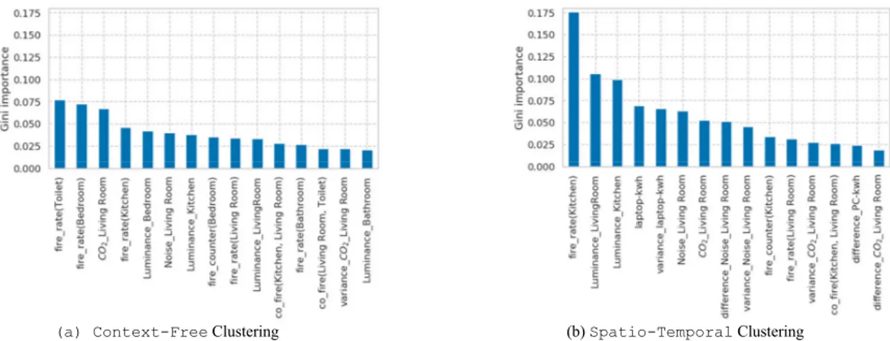
(a) Context-Free Clustering (b) Spatio-Temporal Clustering
applied to generate the feature set of each contextual (i.e., context-aware or context-free) approach. In the rest of this section, we aim to give an overview of this feature set and how this set differs among the different approaches. For brevity, we discuss only the generated feature set of the Context-Free approach and we contrast it with the feature set generated for the Spatio-Temporal approach. However, similar observations can be made for the rest of the considered approaches.
Fig. 2a illustrates the top-15 features (x-axis), as ranked by
Gini-Importance (y-axis), when considering the entire feature
space (see Section III-B). The top-15 features formalize the feature set of the Context-Free approach. We notice that half of these features concern sensor data derived by a sensor located either at the kitchen or at the living room. This observation can be explained, if we consider that the majority of daily-life activities are taking place in those rooms. Thus, these features are better suited to predict said activities.
Fig. 2b illustrates the top-15 features (x-axis), as ranked by
Gini-Importance (y-axis), when considering the
spatio-temporal context (𝑅 Kitchen/Living Room, 𝑇 afternoon). We notice that when the context is specified, more fine-grained features (e.g., laptop-kwh) are included in the feature set. These features are more probable predicting activities related to a particular spatio-temporal context (e.g., resting).
D. Evaluation
In this section, we provide a thorough investigation of our proposed approaches, both from the performance and time scalability perspective. All the experiments were conducted on a 2.40 GHz Intel(R) Xeon(R) CPU E5-2680 v4 processor with 132 GB memory and running on an Ubuntu 16.04.5 operating system. We use 33% of the annotated dataset for feature selection and creating initial clustering for algorithms, while the rest as stream data. We split the temporal dimension 𝑇 into 4 periods, namely morning (06:30-12:29), noon (12:30-18:29),
afternoon (18:30-00:29), night (00:30-06:29). The spatial
dimension 𝑅 is divided into four rooms, namely Kitchen/Living
Room, Bedroom, Toilet, and Bathroom.
The performance of these approaches is evaluated using unsupervised and supervised measures. For unsupervised evaluation, the average Silhouette Coefficient [7] measure is utilized. Intuitively, it measures how well a data point fits in the assigned cluster, compared to how well it would fit in the nearest cluster. Its value varies between -1 to 1 and the higher the value, the better is the quality of the output.
In the case of supervised evaluation, a variation [13] of the traditional measures, Precision, Recall, and F-Measure, is implemented. This variation is adapted to a clustering, where neither the number of clusters nor the
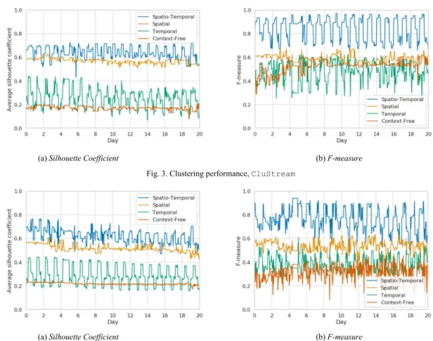
(a) Silhouette Coefficient (b) F-measure Fig. 3. Clustering performance, CluStream
(a) Silhouette Coefficient (b) F-measure Fig. 4.Clustering performance, MiniBatch k-means
mapping between known classes in the ground truth (generated by annotations) and clusters are known.
1) Clustering Performance
Fig. 3 illustrates the performance (y-axis) of different proposed approaches with respect to time (x-axis) using the CluStream algorithm. Fig. 3a, in particular, shows the average Silhouette Coefficient (y-axis), generated by each of the proposed approaches on different days (x-axis). Overall, context-aware approaches exhibited a better performance than the context-free approach. This result confirms our initial intuition that modeling contextual information can positively impact the quality of HAR.
Spatial CluStream reaches a performance close to 60% of the average Silhouette Coefficient, indicating the ability of the spatial context to detect daily-life activities. By contrasting its clustering results with the time distribution of the daily-life activities, we arrived at a key observation. Spatial CluStream is able to detect activities occurring concurrently in different rooms, such as bathing and cooking, without making any a priory assumption on the duration, place, time, and participants of the activity. However, it lacks the ability to distinguish activities with similar data distributions, even if they occur at different time periods. For instance, visiting and
cleaning have similar distributions of noise, CO2, etc, causing
the algorithm to wrongly cluster them together.
On the contrary, Temporal CluStream does not suffer from this problem. It can unfold temporally independent activities, even if they exhibit the same spatial context (e.g.,
resting and eating in the living room). Moreover, the longer an
activity lasts and the higher its occurrence probability in the same period, the better is the performance of Temporal CluStream. However, this approach suffers from holding apart data of concurrently or sequentially occurring activities,
such as toileting and bathing. This drawback hurts its performance which remains at approximately 30%.
Spatio-Temporal CluStream overcomes the aforementioned limitations and shows promising results. Fig. 3b illustrates the average F-Measure (y-axis) achieved using
all approaches over different days (x-axis).
Spatio-Temporal CluStream benefits from modeling the
dimensions of both contexts, leading to an accuracy of up to 98%. As will be discussed in Section III-D2, Spatio-Temporal CluStream not only distinguishes activities of similar underlying distributions, but also evolves its clusters to absorb the variability in data and dynamically adapts to upcoming changes.
Fig. 4 depicts the performance (y-axis) of various approaches on different days (x-axis), when using MiniBatch k-means. Although observations similar to those noted when using CluStream can be made, there are two significant points that should be mentioned. Firstly, as we do not notice a significant difference in the performance between CluStream and MiniBatch k-means, we can safely assume that the behavior of the various proposed approaches is not affected or favored by any particular clustering algorithm. This gives us to understand that the obtained performance is due to contextual modeling and not due to the clustering ability. Secondly, the performance of MiniBatch k-means, in overall, is slightly worse than that of CluStream. Although the online, streaming CluStream has a limited view of the entire dataset, it seems to adapt better to the variability in IoT data.
2) Variability in Data
In this section, a micro perspective analysis is adopted to help us move from the big picture of clustering performance into the details of each cluster. We delve into studying the intrinsic characteristics of the clusters; size, age, quality, ratio of annotated data and prevailing activity label. Our results demonstrate the utility of the proposed approaches and show the variability in meaning over time.
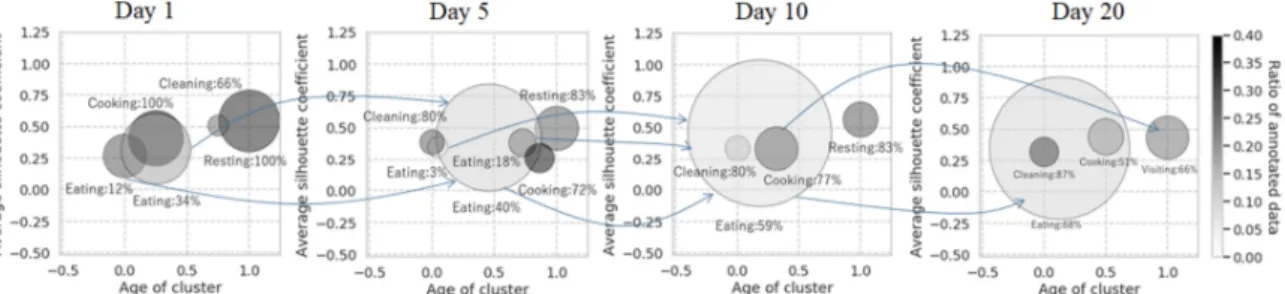
Fig. 5 shows a graphical representation of intrinsic cluster characteristics. Each plot presents clustering during one day, as generated by Spatio-Temporal CluStream, where 𝑅 Kitchen/Living Room and 𝑇 afternoon. We focus our analysis only on this approach as it is considered the most qualitative and representative method. Each plot illustrates clusters, shown as circles; the center of each circle is positioned to pinpoint the quality of the cluster (y-axis) and its age (x-axis). Quality is calculated as the Silhouette Coefficient,
Fig. 5. Variability in data; age (x-axis), quality (y-axis), size (radius), ratio of annotated data (color) and activity label.
while age is the median of all timestamps of the cluster data points. The median is normalized from 0 (oldest) to 1 (newest). For instance, a circle located at the top right corner exemplifies a young and high-quality cluster. Moreover, the size of each circle indicates the number of data points inside a cluster, while color intensity gives the ratio of annotated data to the total number of data within the cluster. For instance, a small dark cluster contains only a few data points, where the majority of them are annotated. For each cluster, a label is assigned representing a daily-life activity. The activity label is assumed to be the one indicated by the majority of annotated data points within that cluster. This assumption is used to facilitate visualization of the activity and enhance the understanding of variability in meaning. Along with the activity label of the cluster, we show the percentage of annotated data with the same label and present in that cluster. The higher the number of annotated data within a cluster, the more confident we are about the activity label. Finally, we draw an arrow between two clusters corresponding to different days to illustrate a change in the meaning of that cluster.
Day 1 shows five clusters, indicating most of the daily-life activities, such as eating, cooking, cleaning, and resting. We notice that the size of the clusters is quite calibrated and a good proportion of annotated data exists per cluster. As the algorithm processes more data over days, the clusters evolve and exhibit new intrinsic characteristics. For instance, the cluster of eating survives and expands in size, appearing also on the 5th and 10th day. Moreover, several smaller clusters of the same label are absorbed by the biggest in size eating cluster. This absorption enhances the confidence of the cluster in detecting the right activity as shown by the increase in the percentage of annotated data (from 34% in Day 1 to 68% in Day 20). Another important observation is derived from the arrow connecting cooking on Day 10 with visiting on Day 20. Note that these two activities exhibit similar underlying distributions (i.e., level of noise and firing rate of motion sensors) and same context (i.e. same 𝑇 and 𝑅 ). Despite the difficulty in distinguishing these two activities, the algorithm is successful in detecting them both. The algorithm dynamically adapts to the changing meaning in data, making itself appropriate for highly varying data.
3) Real-Time Performance
Fig. 6 illustrates the total computational time (y-axis) for all approaches (x-axis), when executing CluStream. The total computational time includes three computational steps (see Algorithm 1)- initialization time (line 1), data processing time (lines 2-14) and macro-cluster generation time (lines 15-17). Note that the latter step is the most time-consuming operation. Overall, the required time for all approaches is below a few minutes for processing data acquired over several days. We notice that Spatio-Temporal requires less time than the rest of the approaches. The reduced calculation time is due to the limited amount of processed data. Further, given its good quality performance, we can conclude that Spatio-Temporal CluStream strikes the best balance between
quality and running time.
Similar observations were made for the computational performance of different approaches while executing MiniBatch k-means (details omitted for brevity). Given that MiniBatch k-means is an offline algorithm, its performance on a particular day is calculated over the dataset accumulated until that day. To this end, the algorithm exhibits an exponential tendency. It is worth mentioning that all approaches require more time, at least an order of magnitude than CluStream for achieving a similar quality of performance. This result encourages the utilization of online streaming algorithms for solving HAR problems.
IV. RELATED WORK
HAR is a well-studied scientific area, which has revealed interesting research questions and remarkable results. Related work in this domain can be mainly organized into two categories- knowledge-driven and data-driven techniques.
Knowledge-driven techniques create models, which a priori capture the contextual information and reason over it to provide valuable insight of where, when, how and by whom each activity is usually performed. Attempts were made to exhaustively model the daily living context is done in [14] and [15]. The authors establish domain-specific ontology associated with each activity to a particular time, location, person or even a sensor. Based on this model and a detailed list of rules on how an activity might be executed, semantic reasoning is applied to infer the activity most likely to occur. Although knowledge-driven approaches are able to model the environmental context and recognize activities using rule-based logic, they are limited by their ability to capture a variety of activity patterns, handling uncertainty, and their comparatively higher computational cost. To overcome these limitations, a different research methodology focusing on data-driven techniques has been developed. These techniques make strategic decisions based on data analysis without any a priori modeling of the particular domain. Probabilistic models and clustering algorithms are among the prevailing techniques for analyzing and predicting HAR. The authors of [16] demonstrate the ability of Markov probabilistic model to recognize activities performed by a single occupant. The authors of [17] go beyond HAR for single occupancy by proposing an extension of Hidden Markov Model (HMM). This extension adds new transition probabilities, which model co-operative activities. The authors of [18] are also exploring HMM for the purpose of recognizing multi-resident activities, while the authors of [19] exploit an enhanced Bayesian network to detect interleaved (or interrupted) activities. Although these approaches have been fairly effective, they are limited to very few types of activities and ignore variability in IoT data over time. This ignorance prevents them from being applied in real-life deployments. Recent works [20] and [21] have shown that when variability exists in data, several drifts (i.e., changes in meaning), may occur at an unprecedented rate. To deal with the challenges of understanding and recognizing these drifts, adaptive clustering should be considered. In our
work, we study a state-of-the-art clustering algorithm [5] which adapts to drifts by adjusting its model to data changes.
Although data-driven techniques strengthen the HAR task, they face with some limitations. Firstly, they induce a comparatively high computational cost depending on the complexity of the utilized model. In our work, we show that the complexity of the proposed model is exclusively dependent on the selection of the clustering algorithm. Secondly, they are craving for training data which should be properly selected in order to represent different domains, activities and actors. In our work, we focus on selecting the appropriate feature space to minimize the impact of the training dataset.
Last but not least, some works [22]–[24] can be found on the borderline interface of knowledge and data-driven techniques. These hybrid approaches are keen on exploiting the advantages of contextual information of knowledge-driven technique and dynamic decision making of data-driven techniques. However, they have not yet completely overcome the limitations of their predecessors.
V. CONCLUSION
To facilitate understanding of variability in IoT data and capture the meaning of HAR, we proposed three contextual approaches. A demonstration of these contextual approaches showed that spatio-temporal approaches have a positive impact on both of calculation time and the quality performance, compared to context-free approaches. This approach resulted in approximately 20% reduction in calculation cost and 20% improvement in accuracy. Further, the online CluStream algorithm strikes the best balance between accuracy and computational cost. We believe that this work lays the foundation for a series of new contributions in exploring variability in IoT data. One direction we are pursuing is the applicability of our approach for the detection of urgent situations in daily living, which are marked by deviations from normal spatial and temporal patterns.
ACKNOWLEDGMENT
This work was partially supported by EU-Activage project Grant No 732679, MEXT/JSPS KAKENHI Grant (B) Number JP16H04455 and JP17H01739, and the Research Grant of Keio Leading-edge Laboratory of Science & Technology.
REFERENCES
[1] F. J. Ordo´n˜ez, P. Toledo, and A. Sanchis, “Sensor-based Bayesian detection of anomalous living patterns in a home setting.” Personal and Ubiquitous
Computing, vol. 19, no. 2, pp. 259–270, Feb. 2015.
[2] N. Goonawardene, X. Toh, and H.-P. Tan, “Sensor-driven detection of social isolation in community-dwelling elderly.” International
Conference on Human Aspects of IT for the Aged Population, Springer, Cham., pp. 378–392., May 2017.
[3] I. de la Torre D´ıez, S. Alonso, S. Hamrioui, E. Cruz, L. Moro´n, and M. Franco, “IOT-based services and applications for mental health in the literature.” Journal of Medical Systems, vol. 43, no. 12 2018.
[4] X. Fan, Q. Xie, X. Li, H. Huang, J. Wang S. Chen, S, … J. Chen, “Activity recognition as a service for smart home: Ambient assisted living application via sensing home.” Proceedings - 2017 IEEE 6th
International Conference on AI and Mobile Services, AIMS 2017, pp. 54–
61.
[5] C. C. Aggarwal, J. Han, J. Wang, and P. S. Yu, “A framework for clustering evolving data streams.” Proceedings of the 29th International Conference
on Very Large Data Bases, VLDB Endowment, vol. 29, pp. 81–92, Sept.
2003.
[6] D. Sculley, “Web-scale k-means clustering.” in Proceedings of the 19th
international conference on World wide web, ACM, pp. 1177–1178, Apr.
2010.
[7] P. J. Rousseeuw, “Silhouettes: a graphical aid to the interpretation and validation of cluster analysis.” Journal of Computational and Applied
Mathematics, vol. 20, pp. 53–65, 1987.
[8] Eclipse sensiNact [Online] Available:
https://projects.eclipse.org/proposals/eclipse-sensinact
[9] M. Yoshida, S. Kleisarchaki, L. Gürgen and H. Nishi, "Indoor Occupancy Estimation via Location-Aware HMM: An IoT Approach." 2018 IEEE
19th International Symposium on "A World of Wireless, Mobile and Multimedia Networks" (WoWMoM), pp. 14-19, June 2018.
[10] P. M. Granitto, C. Furlanello, F. Biasioli, and F. Gasperi, “Recursive fea- ture elimination with random forest for PTR-MS analysis of agroindustrial products.” Chemometrics and Intelligent Laboratory
Systems, vol. 83, no. 2, pp. 83–90, 2006.
[11] L. Breiman, “Random forests.”Machine Learning, vol. 45, no. 1, pp. 5– 32, 2001.
[12] G. Louppe, L. Wehenkel, A. Sutera, and P. Geurts, “Understanding variable importances in forests of randomized trees.” in Advances in
Neural Information Processing Systems, pp. 431–439, 2013.
[13] R. Marxer and H. Purwins, “An f-measure for evaluation of unsupervised clustering with non-determined number of clusters.” Report of the
EmCAP project (European Commission FP6-IST), 1-3, 2008.
[14] L. Chen, C. D. Nugent, and H. Wang, “A knowledge-driven approach to activity recognition in smart homes.” IEEE Transactions on Knowledge
and Data Engineering, vol. 24, no. 6, pp. 961–974, 2012.
[15] J. Ye, G. Stevenson, and S. Dobson, “KCAR: A knowledge-driven approach for concurrent activity recognition.” Pervasive and Mobile
Computing, vol. 19, pp. 47–70, 2015.
[16] G. Singla, D. J. Cook, and M. Schmitter-Edgecombe, “Incorporating temporal reasoning into activity recognition for smart home residents.”
Proceedings of the AAAI Workshop on Spatial and Temporal Reasoning, pp. 53–61, July 2008.
[17] Y.-T. Chiang, K.-C. Hsu, C.-H. Lu, L.-C. Fu, and J. Y.-J. Hsu, “Interaction models for multiple-resident activity recognition in a smart home.” in 2010
IEEE/RSJ International Conference on Intelligent Robots and Systems, IEEE, pp. 3753–3758, Oct. 2010.
[18] R. Chen and Y. Tong, “A two-stage method for solving multi-resident activity recognition in smart environments.” Entropy, vol. 16, no. 4, pp. 2184–2203, 2014.
[19] C.-H. Lu and L.-C. Fu, “Robust location-aware activity recognition using wireless sensor network in an attentive home.” IEEE Transactions on
Automation Science and Engineering, vol. 6, no. 4, pp. 598–609, 2009.
[20] D. Puschmann, P. M. Barnaghi, and R. Tafazolli, “Adaptive clustering for dynamic iot data streams.” IEEE IoT, vol. 4, pp. 64–74, 2017. [21] S. Kleisarchaki, S. Amer-Yahia, A. Douzal-Chouakria, and V.
Christophides, “Querying temporal drifts at multiple granularities.”
Proceedings of the 24th ACM International on Conference on Information and Knowledge Management, ACM, pp. 1531–1540, Oct.
2015.
[22] G. Azkune, A. Almeida, D. Lo´pez-de-Ipin˜a, and L. Chen, “Extending knowledge-driven activity models through data-driven learning tech- niques.” Expert Systems with Applications, vol. 42, no. 6, pp. 3115–3128, 2015.
[23] L. Meng, C. Miao, and C. Leung, “Towards online and personalized daily activity recognition, habit modeling, and anomaly detection for the solitary elderly through unobtrusive sensing.” Multimedia Tools and
Applications, vol. 76, no. 8, pp. 10 779–10 799, 2017.
[24] J. Ye, G. Stevenson, and S. Dobson, “USMART: An unsupervised semantic mining activity recognition technique.” ACM Transactions
on Interactive Intelligent Systems (TiiS), vol. 4, no. 4, pp. 16,