1
Towards adaptive topology optimization
ALEXANDRE NANA, JEAN-CHRISTOPHE CUILLIÈRE*, VINCENT FRANCOIS
Équipe de Recherche en Intégration Cao-Calcul, Université du Québec à Trois-Rivières, 3351 Boulevard des Forges, Trois-Rivières, G9A 5H7, Québec, Canada.
*Corresponding author Jean-Christophe Cuillière [email protected]
Abstract: This paper presents a new fully-automated adaptation strategy for structural topology optimization (TO) methods. In this work, TO is based on the SIMP method on unstructured tetrahedral meshes. The SIMP density gradient is used to locate solid-void interface and h-adaptation is applied for a better definition of this interface and, at the same time, de-refinement is performed to coarsen the mesh in fully solid and void regions. Since the mesh is no longer uniform after such an adaptation, classical filtering techniques have to be revisited to ensure mesh-independency and checkerboard-free designs. Using this adaptive scheme improves the objective function minimization and leads to a higher resolution in the description of the optimal shape boundary (solid-void interface) at a lower computational cost. This paper combines a 3D implementation of the SIMP method for unstructured tetrahedral meshes with an original mesh adaptation strategy. The approach is validated on several examples to illustrate its effectiveness. Keywords: topology optimization, SIMP, adaptation, filtering.
1 Introduction
Topology optimization (TO) of continuum structures [1, 2] is a powerful tool that gradually becomes a key step in the design process of many products and structures. It consists in calculating the optimal distribution of material, with respect to a given objective, in a design domain under sets of constraints. It is becoming a very attractive and important tool in practical engineering [3-5] since it allows producing significantly superior designs and greater savings, than when using parametric optimization or trial and error approaches. Over the past decades, the most widely used TO techniques are the Solid Isotropic Material with Penalization (SIMP) method [6], homogenization based methods [7, 8], level sets based methods [9, 10] and Evolutionary Structural Optimization (ESO) methods [11, 12].
In general terms, the SIMP method consists in determining whether or not a point located inside a given design domain should be solid material. In the SIMP method, the volume fraction is prescribed as an input, and is kept constant throughout optimization iterations. Although optimization results are likely to be enhanced through mesh refinement, this refinement is only required close to its boundary, while interior (fully solid) and exterior (fully void) material can be defined using a coarse discretization. These remarks suggest, as pointed out by Aremu et al. [13], that an adaptive mesh improvement strategy could be incorporated in the SIMP optimization process. This paper develops a new adaptive TO scheme which performs both mesh refinement and de-refinement for 3D optimization problems. The mesh adaptation strategy only refines elements at the boundary of the optimal shape and coarsens elements when moving away from it. Using such an adaptive process improves the boundary shape extraction and reduces POSTPRINT VERSION. The final version is published here :
Nana, A., Cuillière, J.-C., & Francois, V. (2016). Towards adaptive topology optimization. In Advances in Engineering Software (Vol. 100, pp. 290-307). https://doi.org/10.1016/j.advengsoft.2016.08.005 CC BY-NC-ND 4.0
2 subsequent post-processing for the interpretation of TO results. Furthermore, by coarsening the mesh inside and outside the optimized domain, the computational cost of SIMP iterations is expected to considerably decrease. Another potential gain that can be foreseen is increasing the achievable geometric complexity of optimal designs. Indeed, a better definition of the boundary and more geometric complexity are attractive when using TO methods along with additive manufacturing. Moreover, as mentioned in [14], improving the quality of TO results at the design stage, even by a very modest amount, may have a huge impact on the overall cost of products when considering the entire lifespan. It is, for example, the case in aerospace applications, for which a tiny loss in weight induces very important fuel savings along the use of these products.
The paper is organized as follows. In the next section (section 2) we present and discuss previous work related to adaptive TO. Section 3 starts with a short overview of the SIMP method and introduces the concepts on which our mesh adaptation scheme is based. It also shows that classical filtering techniques, that have proven efficiency in preventing numerical instabilities of the SIMP method on uniform meshes, have to be adapted in the context of using highly non-uniform unstructured meshes. Section 3 ends with an analysis of the influence, on optimization results obtained, of the main parameters of our adaptation scheme. In section 4, the effectiveness of our approach is validated through sets of numerical examples. Conclusions are drawn and we sketch some directions for future work in the last section.
2 Related work
Although a limited number of approaches can be found in the literature towards implementing adaptive TO of 3D structures, setting up adaptive schemes to improve optimal solutions is not a new idea. In 1995, Maute and Ramm [15] indeed proposed a method for adapting optimization results in 2D. This methods starts with roughly extracting iso-density curves, which is followed by refining the mesh around these curves and ends with considering this new mesh as a new optimization problem, with the same boundary conditions and loads. By reducing, at each new optimization, the finite element mesh size and increasing the considered value in iso-density curves extraction, several optimization cycles are applied, until reaching a result with satisfying quality. However, this technique is restricted to 2D optimization problems and the overall domain is refined (no de-refinement is carried out). Later, based on the geometrical discretization error, Ramm et al. [16] proposed an h-adaptive strategy for shape optimization. As an extension of their method to topology optimization, they were the first, to our knowledge, to introduce the idea that the spatial gradient of material distribution can be used as a refinement criterion in topology optimization. Costa and Alves [17] refined an initially coarse triangular mesh after a certain number of optimization steps. In their work, the refinement strategy is based on estimating the error on stress distribution. After each refinement, a constrained Laplacian smoothing is applied on the mesh to improve elements quality. Still, both solid and boundary elements are refined and no de-refinement is applied. Roman Stainko [18] first considered only refining the mesh at the solid-void interface and applying it to tetrahedral meshes. In his approach, new elements are inserted only at the boundary of the optimal design and fully solid and void regions are not refined. A filter is introduced in the refinement process to control the number of elements around the solid-void interface and refinement is performed through partial re-meshing. However, no de-refinement is performed. Few years later, Sturler et al. [19] and
3 Wang et al. [20] introduced the AMR (Adaptive Mesh Refinement) concept to achieve the design that would be obtained on a uniformly fine mesh. Their dynamic mesh refinement and de-refinement is performed continuously throughout the optimization process, but de-refinement and de-refinement are not carried out simultaneously. Moreover, both solid-void interface and solid volume are refined, which is likely to refine the mesh where it doesn’t necessarily need to be. Bruggi et al. [21] propose a modified version of this approach that is driven by two error estimators and for which de-refinement is only performed inside the void region and at the last adaptive step. In this approach, the first error estimator used is related to the amplitude of intermediate regions (solid-void interface) and the second one is related to the FEA error itself. More recently, Duan et al. [22] introduce an adaptive mesh refinement strategy for TO applied to computational fluid dynamics (CFD) for which refinement is driven by distance to the boundary. Wang et al. [23] propose using two separate discretizations along TO : one discretization for approximating the relative density field and the other one for FEA. The relative density mesh is refined with respect to optimization results while the analysis mesh is refined with respect to FEA error estimation. The advantage is that it guarantees that refinement based on the relative density field does not degrade analysis results. However, the method does not feature any de-refinement process and requires using non-conventional finite elements (so-called level-one mesh
incompatibility [20]). Being able to use conventional finite elements is indeed an advantage since
it basically allows using any FEA solver. Lin et al. [24] performed a two-stage TO algorithm for homogenization methods where the optimal design obtained at the end of the first optimization stage is projected on a refined uniform mesh, which is then used as the initial topology for the second stage of the optimization. Another alternative to improve TO results by combining adaptive meshing strategy and (Bi)directional ESO (so-called BESO) scheme is proposed by Aremu et al. [25] to solve a standard cantilever beam. During the re-meshing process, elements are refined using two refinement templates by bisection and mesh coarsening is performed through edge collapsing. However, this strategy degrades mesh quality and it may not be straightforward to extend it to 3D optimization problems. Similarly, Liu et al. [26] couples an adaptive moving mesh method (also called r-adaptivity scheme) with a level set TO scheme. Unlike previous re-meshing and updating procedures, they updated mesh grid points following topology changes to better approximate the optimal shape without changing the mesh topology. Furthermore, large deformation problems with meshfree analysis in TO design have been addressed by He et al. [27]. They have obtained good optimal solutions without mesh difficulties and numerical instabilities by using an element-free Galerkin method, which represents a promising and interesting alternative to FEA based optimization.
Topology optimization capabilities have been successfully implemented in several commercial systems [28, 29]. TOSCA is a commercial TO solution that features an adaptive mesh refinement during the TO process. However, this commercial implementation is limited [14]. In the current version, the adaptive process is limited to two refinement iterations and mesh refinement is implemented using templates based on 2D quad elements that are not straightforward to extend to the general context of unstructured tetrahedral meshes.
As a conclusion, the aforementioned methods are either limited to 2D optimization problems and/or do not feature a de-refinement process. It also appears that, since mesh density strongly influences both the computational cost of TO and the smoothness and accuracy in the description
4 of the optimal shape, mesh adaptation is a potentially very useful tool in the improvement of TO results. This is why, in this paper, we present a fully-automated adaptive TO scheme that includes simultaneous mesh refinement and de-refinement and that applies on 3D unstructured tetrahedral meshes.
3 A new adaptive topology optimization process
As introduced in the previous section, our objective is simultaneously refining and de-refining specified regions of finite element meshes used in TO to improve accuracy in the definition of optimal shape boundary at a low computational cost.
3.1 The SIMP Method 3.1.1 Basic principles
The SIMP (Solid Isotropic Material with Penalization) method is based on considering an artificial solid isotropic material with power-law penalization of intermediate densities to steer the optimal solution to a discrete 0-1 design (0 density stands for void and 1 density for full material). Thus, from SIMP results (a distribution of density across the mesh that represents design material) the optimal design shape is obtained from sets of finite elements with a density that is close to 1. In this paper, the implementation of the SIMP method used consists in optimizing the distribution of a fixed amount of material inside the design volume towards minimizing its global compliance (or flexibility), which generally means maximizing its stiffness. The distribution of material inside the design volume is represented by a relative density distribution 𝜌(𝑥, 𝑦, 𝑧), which is updated along finite element iterations. Convergence of SIMP iterations is achieved when the relative difference in global compliance between two successive iterations is less than a given threshold.
In classical implementations of the SIMP method, 𝜌(𝑥, 𝑦, 𝑧) is a scalar that is constant per element (𝜌𝑒 in element 𝑒). This relative density distribution is related to the distribution of a
virtual elastic modulus 𝐸 according to the penalization law:
𝐸̃(𝑥, 𝑦, 𝑧) = 𝐸 ∙ (𝜌(𝑥, 𝑦, 𝑧))𝑝 (1)
Where 𝑝 is a penalization coefficient (𝑝 = 3 in this work).
In the following equations, as for the elastic modulus 𝐸̃(𝑥, 𝑦, 𝑧), all objects that are affected by the relative density field 𝜌(𝑥, 𝑦, 𝑧) are noted using a ~. For example, if [𝐾𝑒] is the local stiffness
matrix of element 𝑒, [𝐾̃𝑒] will be the local stiffness matrix [𝐾𝑒] affected by the relative density
field 𝜌(𝑥, 𝑦, 𝑧). Once 𝐸̃(𝑥, 𝑦, 𝑧) is calculated from 𝜌(𝑥, 𝑦, 𝑧), the global stiffness matrix [𝐾̃] is assembled from local stiffness matrices [𝐾̃𝑒] (for 𝑁 finite elements 𝑒):
[𝐾̃] = 𝛢𝑒=1𝑁 [𝐾̃
𝑒] = 𝛢𝑁𝑒=1(𝜌𝑒(𝑥, 𝑦, 𝑧))𝑝∙ [𝐾𝑒] (2)
where 𝛢𝑒=1𝑁 refers to the finite element assembly operator (scattering and adding elementary
5
𝜌𝑒 is the relative density inside element e
The TO problem is classically formulated as follows:
{ 𝑚𝑖𝑛 𝐶̃ ={𝑈̃}𝑡∙ [𝐾̃] ∙ {𝑈̃} 𝑠. 𝑡. { [𝐾̃] ∙ {𝑈̃} = {𝐹} 𝑉̃ 𝑉𝑑 = 𝑓 𝐸̃(𝑥, 𝑦, 𝑧) = 𝐸 ∙ (𝜌(𝑥, 𝑦, 𝑧))𝑝 0 < 𝜌𝑣𝑜𝑖𝑑 ≤ 𝜌 ≤ 1 (3)
It consists in minimizing the compliance 𝐶̃ while maintaining constant the volume fraction 𝑓. The volume fraction is defined as the ratio between volume 𝑉̃ (affected by 𝜌(𝑥, 𝑦, 𝑧)) and the initial design volume 𝑉𝑑. {𝑈̃} is the global displacement vector (affected by 𝜌(𝑥, 𝑦, 𝑧)) and the
global load vector is {𝐹}.
For each SIMP iteration, the relative density field 𝜌 is updated modified using the Optimality Criteria (OC) algorithm. Thus, 𝜌𝑒 is modified using:
𝜌𝑒𝑛𝑒𝑤 = {
max (𝜌𝑣𝑜𝑖𝑑, 𝜌𝑒 − 𝑚) 𝑖𝑓 𝜌𝑒𝛽𝑒𝜂 ≤ max (𝜌𝑣𝑜𝑖𝑑, 𝜌𝑒− 𝑚)
𝜌𝑒𝛽𝑒𝜂 𝑖𝑓 max(𝜌𝑣𝑜𝑖𝑑, 𝜌𝑒− 𝑚) < 𝜌𝑒𝛽𝑒𝜂 < min (1, 𝜌𝑒+ 𝑚) min (1, 𝜌𝑒+ 𝑚) 𝑖𝑓 min(1, 𝜌𝑒+ 𝑚) ≤ 𝜌𝑒𝛽𝑒𝜂
}
where 𝜌𝑒 is the previous relative density inside element e and 𝜌𝑒𝑛𝑒𝑤 is the updated (or new)
relative density inside element e
𝑚 is a threshold on the variation of 𝜌𝑒 and consequently |𝜌𝑒𝑛𝑒𝑤− 𝜌
𝑒| ≤ 𝑚 (practically, we used
𝑚 = 0.2 for the examples presented in this paper 𝜂 = 1
2 is a damping coefficient
𝜌𝑣𝑜𝑖𝑑 corresponds to a “numerical” void (for the results presented, the practical value of 𝜌𝑣𝑜𝑖𝑑
is 10−3). It is used to avoid numerical singularities.
e is calculated using the following equation:
𝛽𝑒 = −𝜕𝜌𝜕𝐶̃ 𝑒 𝜆𝜕𝜌𝜕𝑉̃ 𝑒 𝜕𝐶̃
𝜕𝜌𝑒 is the global compliance’s sensitivity with respect to 𝜌𝑒, calculated from:
𝜕𝐶̃ 𝜕𝜌𝑒
= − 𝑝 𝜌𝑒
. {𝑈̃}𝑡. [𝐾̃𝑒]. {𝑈̃}
Practically, {𝑈̃}𝑡. [𝐾̃𝑒]. {𝑈̃} is provided by FEA results, using the total strain energy inside element e, 𝑊̃𝑒 :
6 𝑊̃𝑒 =1 2. {𝑈̃} 𝑡 . [𝐾̃𝑒]. {𝑈̃} Consequently: 𝜕𝐶̃ 𝜕𝜌𝑒 = − 2. 𝑝. 𝑊̃𝑒 𝜌𝑒 From 𝑉̃ = ∑ 𝑉̃𝑁𝑒=1 𝑒 = ∑𝑁𝑒=1 𝜌𝑒. 𝑉𝑒 we calculate 𝜕𝑉̃ 𝜕𝜌𝑒= 𝜕𝑉̃𝑒 𝜕𝜌𝑒= 𝑉𝑒 which leads to 𝛽𝑒 = 2.𝑝.𝑊̃𝑒 𝜆.𝜌𝑒.𝑉𝑒
is a Lagrange multiplier, which is calculated from applying bisection iterations. These iterations adjust the value of so that the volume fraction constraint is satisfied:
𝑉̃(𝜌) = ∑ 𝜌𝑒𝑛𝑒𝑤. 𝑉𝑒 𝑁
𝑒=1
= 𝑓. 𝑉𝑑
3.1.2 Filtering sensitivity and density
It is well known that to obtain macroscopic void-solid solutions for the optimized domain some sort of global or local restriction on the variation of density must be imposed in the TO problem [1]. Obtaining checkerboard-free solutions is classically achieved by using a mesh-independency filter, which consists in modifying the design sensitivity 𝜕𝐶̃
𝜕𝜌𝑒 of element 𝑒 based on a weighted
average of element sensitivities in its neighbourhood [30]:
𝜕𝐶̃ 𝜕𝜌𝑒 = 1 𝜌𝑒⁄𝑉𝑒∙ ∑ 𝐻𝑣∙𝜕𝐶 ̃ 𝜕𝜌𝑣∙𝜌𝑣⁄𝑉𝑣 𝑁𝑒 𝑣=1 ∑𝑁𝑒𝑣=1𝐻𝑣 (4) Where 𝐻𝑣 is a weighting factor given by:
𝐻𝑣 = 𝑟𝑚𝑖𝑛𝑐− 𝑑𝑖𝑠𝑡(𝑒, 𝑣) ; {𝑣 ∈ 𝑁𝑒 | 𝑑𝑖𝑠𝑡(𝑒, 𝑣) ≤ 𝑟𝑚𝑖𝑛𝑐}, 𝑒 = 1, … , 𝑁 (5)
In this expression, 𝑟𝑚𝑖𝑛𝑐 is the sphere radius used to evaluate neighbourhood (𝑁𝑒 elements)
around element 𝑒 and 𝑑𝑖𝑠𝑡(𝑒, 𝑣) is the distance between the centre of elements 𝑒 and 𝑣. This type of filter is purely heuristic but it has proven to be effective in many contexts [1, 21, 31]. Since the refinement process is based on the relative density gradient 𝑔𝑟𝑎𝑑⃗⃗⃗⃗⃗⃗⃗⃗⃗⃗ (𝜌), the relative density distribution around each element 𝑒 also needs to be filtered after each SIMP iteration. Indeed, we need 𝑔𝑟𝑎𝑑⃗⃗⃗⃗⃗⃗⃗⃗⃗⃗ (𝜌) to be as continuous as possible, which is achieved by filtering the relative density distribution 𝜌(𝑥, 𝑦, 𝑧) as classically used in some implementations of the SIMP method [1]. Filtering 𝜌(𝑥, 𝑦, 𝑧) is performed by computing a weighted average of element densities 𝜌𝑣 around element 𝑒. Similar to 𝑟𝑚𝑖𝑛𝑐, this other neighbourhood around element 𝑒 is
represented by sphere with radius 𝑟𝑚𝑖𝑛𝑑 and density 𝜌𝑒 is modified using [30]:
𝜌𝑒 ̅̅̅ =∑𝑁𝑒𝑣=1𝜔𝑣∙𝜌𝑣 ∑𝑁𝑒𝑣=1𝜔𝑣 with 𝜔𝑣 = 𝑉𝑣∙ 𝑒𝑥𝑝[−12∙(𝑑𝑖𝑠𝑡(𝑒,𝑣)𝑟𝑚𝑖𝑛𝑑 3 ) 2 ] 2𝜋∙(𝑟𝑚𝑖𝑛𝑑3 ) (6)
7 The effect of each filter can be independently controlled by enlarging or shrinking the associated radius. In this paper, values for 𝑟𝑚𝑖𝑛𝑐 and 𝑟𝑚𝑖𝑛𝑑 are taken around 1.25 times the prescribed local
element size (𝑟𝑚𝑖𝑛𝑐 = 𝑟𝑚𝑖𝑛𝑑 = 𝑟𝑚𝑖 𝑛) and both filters (on the sensitivity and the density) are
applied at each step of the SIMP iterative process. This process stops when the relative difference on the global compliance between two successive iterations ∆𝑖 =
𝐶̃𝑖−𝐶̃𝑖−1
𝐶̃𝑖−1 (𝐶̃𝑖 is the
global compliance at iteration i) is less than a threshold ∆𝑐𝑜𝑛𝑣. The final compliance (the
compliance at convergence of SIMP iterations) is noted 𝐶̃𝑓𝑖𝑛𝑎𝑙.
As explained with details in [32], deriving an optimal shape from SIMP results (a relative density distribution 𝜌(𝑥, 𝑦, 𝑧)) is based on a density threshold 𝜌𝑡ℎ. Globally, the optimized shape is made
with design material for which 𝜌(𝑥, 𝑦, 𝑧) > 𝜌𝑡ℎ. We implemented our own SIMP engine, based
on previous work about the SIMP method [1, 31, 33-36] and based on equations 1 to 6. More details about our implementation of the SIMP method can be found in [32].
3.1.3 SIMP results obtained on a sample part
Figure 1a shows the initial geometry of a bike suspension rocker, which is used to illustrate our adaptive TO process, with boundary conditions (the 2 lower bores are fixed) and loads applied (on the 2 upper bores in the 𝑌 direction). The initial rocker overall dimensions are 390 𝑚𝑚 (height), 240 𝑚𝑚 (width) and 32 𝑚𝑚 (thickness). Young’s modulus is 69 GPa and Poisson’s ratio is 0,33. As seen in the SIMP result presented in Figure 1b, non-design material is distributed around the 4 bores. In this example, we used a uniform mesh size 𝑑𝑔 = 3,5 𝑚𝑚, and
both filters were applied, using the same radius 𝑟𝑚𝑖𝑛 = 1,25 ∙ 𝑑𝑔. The volume fraction is 𝑓 =
0,3, the convergence criterion is 𝛥𝑖 < ∆𝑐𝑜𝑛𝑣= 0,5% and the optimal shape is based on the
density threshold 𝜌𝑡ℎ = 0,45. This value of 𝜌𝑡ℎ is chosen with respect to the targeted volume
fraction, which means to the targeted optimized design volume. In general, at the end of the SIMP process, we have observed, through many SIMP optimization cases, that the optimized
design volume is close to the targeted design volume (defined as 𝑓. 𝑉𝑑 according to equation 3)
when 𝜌𝑡ℎ is taken between 0,4 and 0,5.
The raw SIMP result obtained (a relative density distribution 𝜌(𝑥, 𝑦, 𝑧) at the end of SIMP iterations) is illustrated in Figure 1b. From this distribution, the gradient of 𝜌(𝑥, 𝑦, 𝑧) is then computed, which is the base of the adaptive refinement process presented in the next section. The gradient reaches maximum values (which means high variations of the relative density) at the interface between void and solid material in the optimized shape and decreases with the distance to this interface (Figure 1c). Consequently, the relative density gradient is likely to be used as a base for mesh refinement and de-refinement around this interface.
8
Figure 1 : Bike suspension rocker model with (a) loads applied and boundary conditions, (b)
relative density distribution at the end of SIMP iterations with a uniform mesh size 𝑑𝑔 = 3,5 𝑚𝑚
and (c) gradient of the density derived: high values (light-blue) and zero gradient (dark-blue).
3.2 A new adaptive refinement and de-refinement strategy
The basic objective of mesh refinement and de-refinement in TO is reducing the size of the analysis model while improving accuracy in the definition of the optimal shape boundary. The method aims at refining the mesh around the solid-void interface only by using standard finite elements. Unlike [17, 19, 21] where both fully solid and boundary regions are refined, in this work only the solid-void interface is refined while void as well as fully solid regions are coarsened. Moreover, refinement/de-refinement is carried out at the same time for substantial efficiency.
3.2.1 Automatic identification of the optimal shape boundary
As introduced in section 2.1.2., boundaries of the optimal shape can easily be identified from the norm of relative density gradient ‖𝑔𝑟𝑎𝑑⃗⃗⃗⃗⃗⃗⃗⃗⃗⃗ (𝜌)‖. Since in SIMP results, as illustrated in Figure 1b, the relative density field 𝜌(𝑥, 𝑦, 𝑧) is discontinuous (it is a scalar field that is constant within each element), the gradient cannot be computed as is. Before computing the gradient, the discontinuous field 𝜌(𝑥, 𝑦, 𝑧) is transformed into a continuous field, referred to as 𝜌∗(𝑥, 𝑦, 𝑧),
using a classical weighted average computation at each node. Then, the norm of the relative density gradient is practically obtained by calculating ‖𝑔𝑟𝑎𝑑⃗⃗⃗⃗⃗⃗⃗⃗⃗⃗ (𝜌∗)‖. Since this gradient decreases
with distance to the boundaries, it can be used as a good criterion for mesh refinement and de-refinement. As shown in Figure 1c, the gradient is close to 0 inside void and fully solid regions and reaches a maximum value at the solid-void interface. This gradient gives similar, but more accurate results in the detection of the solid-void interface than the user-specified transitional zone thresholds proposed in [23, 37], or with the radius used in [18, 20]. Moreover, alike filter radius 𝑟𝑚𝑖𝑛 used to obtain macroscopic discrete results (see sub-section 3.1.1), [23, 37] also
introduce influence zones around computational points (so-called cut-off radius). These zones are adaptively refined through optimization iterations with the objective of reducing intermediate density zones and therefore improving quality in the representation of structural boundaries. This
9 refinement of density points is based on using square cells. In our work, this type of refinement is based on using 3D tetrahedral elements.
3.2.2 Effect of the mesh size on optimization results and on the relative density gradient
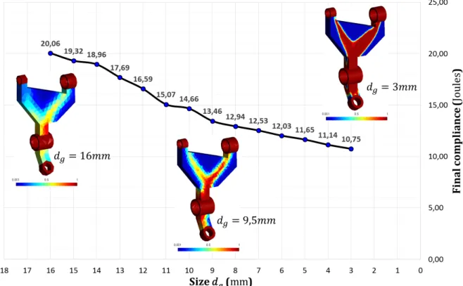
Using a finer mesh obviously increases accuracy in the definition of the optimal shape and leads to a lower final compliance 𝐶̃𝑓𝑖𝑛𝑎𝑙. This is due to a higher number of elements for describing the
density distribution. Figure 2, shows the evolution of the final compliance obtained, for the example introduced in Figure 1, when using uniform meshes with increasing element size (𝑑𝑔varies from 3 𝑚𝑚 to 16 𝑚𝑚). It also shows 3 final relative density distributions at the end of
the optimization process for 𝑑𝑔 = 3 𝑚𝑚, 9,5 𝑚𝑚 and 16 𝑚𝑚. For all these optimizations, the
same value is considered for the convergence criterion (𝛥𝑖 < ∆𝑐𝑜𝑛𝑣= 0,5%). As expected, it
appears that 𝐶̃𝑓𝑖𝑛𝑎𝑙 decreases with element size.
Figure 2 : Evolution of the final compliance 𝐶̃𝑓𝑖𝑛𝑎𝑙 with the mesh size for uniform meshes.
For the same meshes and on the same example (bike suspension rocker), Figure 3 shows the evolution of the maximum gradient obtained with increasing element size (𝑑𝑔 still varies from
3 𝑚𝑚 to 16 𝑚𝑚). This figure reveals that the norm of the maximum gradient globally decreases with element size and that the global trend of this variation is exponential (the dashed line in Figure 3). Since an analogous variation has been observed on other topology optimization problems, this global trend can then be used to set up a refinement and de-refinement strategy that is based on the norm of the relative density gradient as presented in the next section.
10
Figure 3 : Relationship between the norm of maximum relative density gradient and element size for uniform meshes.
3.2.3 Automatic and adaptive mesh refinement and de-refinement
The refinement and de-refinement strategy presented in this paper is based on the computation of an adapted mesh sizing function 𝑑𝑗(𝑥, 𝑦, 𝑧) from the previous optimization results (at step 𝑗 − 1).
The objectives underlying this adapted mesh sizing function is generating coarser elements inside solid and void material and finer elements at the solid-void interface. Moreover, the SIMP process requires meshes with reasonably good element quality, which imposes additional constraints on mesh refinement and de-refinement. Last but not least, the mesh adaptation process needs to be automatic and generic enough to avoid unpractical and time-consuming user interventions. In our adaptation approach, the relative density distribution at the end of a given SIMP optimization procedure is used as an input to generate the adaptive mesh for the next SIMP optimization. In fact, at the beginning of our adaptive strategy, the entire domain is initially uniformly meshed with relatively coarse finite elements and the first SIMP optimization is performed. Using the raw result (a distribution of the relative density 𝜌(𝑥, 𝑦, 𝑧) across the whole mesh) of the first SIMP optimization, norm of the relative density gradient ‖𝑔𝑟𝑎𝑑⃗⃗⃗⃗⃗⃗⃗⃗⃗⃗ (𝜌)‖ is computed in order to identify zones to be refined and zones to be de-refined. Thus, a new mesh sizing function is calculated and an adapted mesh is generated, according to this sizing function, across the whole domain.
In following paragraphs, 𝑑𝑗(𝑥, 𝑦, 𝑧) refers to the mesh sizing function used at the jth refinement
and de-refinement step. The refinement and de-refinement strategy proposed in this paper is based on the following guidelines:
The mesh sizing function used for the first SIMP optimization (step 0) is constant. It is noted 𝑑0(𝑥, 𝑦, 𝑧) = 𝑑𝑔.
11 𝑑𝑗(𝑥, 𝑦, 𝑧) should be maximum and higher than the initial mesh size 𝑑𝑔 where the norm
of relative density gradient, at step 𝑗 − 1, noted ‖𝑔𝑟𝑎𝑑⃗⃗⃗⃗⃗⃗⃗⃗⃗⃗ (𝜌𝑗−1(𝑥, 𝑦, 𝑧))‖, is close to 0.
𝑑𝑗(𝑥, 𝑦, 𝑧) should be minimum where ‖𝑔𝑟𝑎𝑑⃗⃗⃗⃗⃗⃗⃗⃗⃗⃗ (𝜌𝑗−1(𝑥, 𝑦, 𝑧))‖ is maximum.
𝑑𝑗(𝑥, 𝑦, 𝑧) should vary smoothly enough so that a reasonable element quality is achieved.
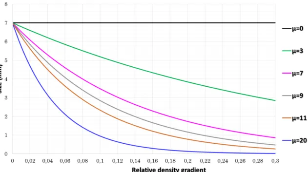
The refinement and de-refinement strategy is based on an exponential function to ensure that the prescribed element size never reaches null values. The targeted element size distribution 𝑑𝑗(𝑥, 𝑦, 𝑧) at refinement and de-refinement step 𝑗 is obtained from the distribution
‖𝑔𝑟𝑎𝑑⃗⃗⃗⃗⃗⃗⃗⃗⃗⃗ (𝜌𝑗−1(𝑥, 𝑦, 𝑧))‖ using:
{
𝑑𝑗(𝑥, 𝑦, 𝑧) = 𝑑𝑔 𝑓𝑜𝑟 𝑗 = 0 𝑑𝑗(𝑥, 𝑦, 𝑧) = 𝐸𝑛𝑚𝑒−µ‖𝑔𝑟𝑎𝑑⃗⃗⃗⃗⃗⃗⃗⃗⃗⃗⃗ (𝜌𝑗−1(𝑥,𝑦,𝑧))‖ 𝑓𝑜𝑟 𝑗 > 0
(7)
𝐸𝑛𝑚 stands for the maximum element size allowed and it is usually higher than the initial uniform mesh size used 𝑑𝑔. µ is a coefficient that controls refinement and de-refinement severity
as illustrated in Figure 4 (with 𝐸𝑛𝑚 = 7 𝑚𝑚).
Figure 4 : Evolution of the prescribed element size with ‖𝑔𝑟𝑎𝑑⃗⃗⃗⃗⃗⃗⃗⃗⃗⃗ (𝜌𝑗−1)‖ for different values of µ.
Unlike alternative approaches such as coarsening by collapsing element edges as proposed in [25] or the application of refinement and de-refinement in two different steps as carried out by [20, 21], we propose a h-type adaptive process for which refinement and de-refinement are performed simultaneously. This is done by re-meshing the entire design domain after each SIMP process is completed. The major advantage in doing that is that it avoids substantial post-processing and mesh incompatibility (as in [23]) and guarantees a much better mesh quality in the adaptation.
12 3.2.4 Numerical implementation
The proposed adaptive TO strategy is implemented and integrated in the Linux based CAD-FEA-TO research platform developed by our team [32]. This platform features integrated modelling, analysis and TO capabilities. It is based on C++ code, on Open CascadeTM [38]
libraries and on the use of Code_AsterTM [39] as FEA solver. In all the figures shown in this
paper, we use GmshTM [40] for visualizing meshes and SIMP results. All optimizations presented
in this paper are performed on a desktop computer with a 3.40 GHz processor with 16 GB RAM. Each result at the end of SIMP iterations is presented as a relative density distribution 𝜌(𝑥, 𝑦, 𝑧), which is a scalar field that is constant within each finite element.
The adaptive TO process starts with an initial CAD model on which material data, boundary conditions (BCs) and loads are applied. Design and non-design sub-domains are also defined on this initial CAD model. The non-design sub-domain refers to the material that should not be affected by the optimization process. A relatively coarse mesh (with constant mesh size 𝑑0(𝑥, 𝑦, 𝑧) = 𝑑𝑔) is first generated on the initial CAD model and a first SIMP optimization is
performed, based on this initial mesh. As explained above in sub-section 3.2.3., a new mesh sizing function 𝑑1(𝑥, 𝑦, 𝑧) is computed from 𝜌0(𝑥, 𝑦, 𝑧), the result of this first SIMP
optimization. A new adapted mesh is generated from 𝑑1(𝑥, 𝑦, 𝑧) and a new SIMP optimization is
then performed using this mesh. As for the second SIMP optimization (after the first adaptation), the third SIMP optimization (after the second adaptation) is performed using a new adapted mesh sizing function 𝑑2(𝑥, 𝑦, 𝑧) computed from 𝜌1(𝑥, 𝑦, 𝑧), the result of the second SIMP
optimization. This adaptive process continues and, by the way, the mesh is gradually and simultaneously refined and de-refined along SIMP optimizations (referred to using subscript j). Of course, each SIMP optimization itself involves FEA iterations (referred to using subscript i). One interesting aspect in the process is that, as suggested in [23], the convergence criterion ∆𝑐𝑜𝑛𝑣evolves along successive SIMP optimization. Indeed, there is no need in achieving a very strict convergence in the first SIMP optimization since the process is adaptive. Thus the convergence criterion used for the jth SIMP optimization, noted ∆
𝑐𝑜𝑛𝑣
𝑗 , decreases with j.
Figure 5 shows SIMP solutions obtained (for the same part as in Figure 1 and for the same material and conditions) after different steps of mesh refinement and de-refinement. Figure 5a shows the SIMP result obtained from the initial uniform relatively coarse mesh (with 𝑑𝑔 =
3,5 𝑚𝑚). For all SIMP iterations, both sensitivity and density filters are applied with the same radius 𝑟𝑚𝑖𝑛= 1,25 ∙ 𝑑𝑗(𝑥, 𝑦, 𝑧). The convergence criterion decreases along SIMP
optimizations: ∆𝑐𝑜𝑛𝑣0 = 2 % for the first SIMP, ∆1𝑐𝑜𝑛𝑣= 0,8 % for the second and ∆𝑐𝑜𝑛𝑣2 = 0,32 %
for the last SIMP. Minimum and maximum values for the imposed mesh size distributions are 1,82 𝑚𝑚 − 7 𝑚𝑚 for 𝑑1(𝑥, 𝑦, 𝑧) after the first mesh adaptation (Figure 5b), and 1,00 𝑚𝑚 −
7 𝑚𝑚 for 𝑑2(𝑥, 𝑦, 𝑧) after the second mesh adaptation (Figure 5c). As shown in Table 1 and
contrary to what could be expected, the final compliance does not decrease along mesh adaptations. This suggests that the adaptive process degrades the optimal shape description instead of improving it. A closer look at Figure 5 confirms that mesh adaptation does not have the expected effect on optimization results since optimal shapes are completely different from one SIMP optimization to the next.
13
Number of
tetrahedra Number of iterations Optimization time (s)
SIMP convergence criterion (%) Compliance (Joules) Initial mesh 169 962 11 298 2,00 11,60 1st adaptation 84 258 14 152 0,80 14,35 2nd adaptation 75 859 16 147 0,32 13,39 Total 41 597
Table 1 : Adaptive topology optimization data results after three SIMP processes and two mesh adaptations for the bike suspension rocker shown in Figure 5.
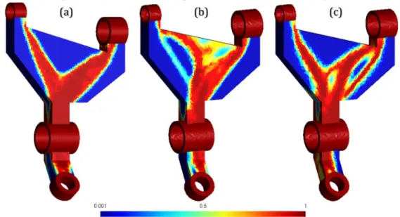
Figure 5 : Relative density distribution at the end of SIMP iterations obtained with (a) a uniform
and relatively coarse mesh 𝑑𝑔 = 3,5 𝑚𝑚, and after (b) the first and (c) the second mesh
adaptation.
3.2.5 A new definition of neighbouring for sensitivity and density filters
Investigations based on several sample parts with different sets of SIMP parameters made us understand that this problem comes from the fact that classical filtering schemes used for uniform or quasi-uniform meshes [31, 35, 36] do not apply anymore when using adapted meshes. The reason is that these adapted meshes locally feature strong variations in mesh size distribution. This implies that the classical neighbourhood used when filtering sensitivity and density, based on a sphere with radius 𝑟𝑚𝑖𝑛 around element e, does not apply in this context and
14
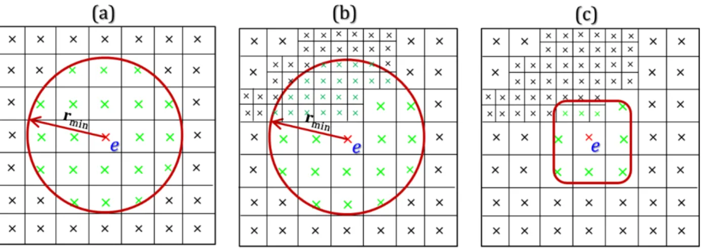
Figure 6 : Neighbouring elements (in green) to element e as considered in sensitivity and density filtering (a) when using a circle on a uniform mesh, (b) when using a circle after mesh
adaptation and (c) when using the first layer of neighbours as in this paper.
Actually, as schematically illustrated in Figure 6 for a 2D quad mesh, neighbouring around element e based on a circle (with radius 𝑟𝑚𝑖𝑛) works well with uniform or quasi-uniform meshes
(Figure 6a). When this type of neighbouring is used for highly graded meshes (Figure 6b) it clearly shows that an inconsistent set of elements around element e will be considered for filtering. Thus, non-uniform unstructured meshes require replacing neighbouring based on circles (in 2D) and spheres (in 3D) by neighbouring by element layers. We consider that two mesh elements are first neighbours if they share a face, an edge or a node. Thereby, a first layer of elements around a given element 𝑒, can be defined (referred to as the first neighbourhood of element 𝑒) by including all elements that are first neighbours of element 𝑒 (in green in Figure 6c). This new definition of neighbouring around element 𝑒 is anisotropic if compared to using a radius, which makes it more consistent with highly graded meshes.
The first neighbourhood (Figure 6c) is used for filtering sensitivity and density in Figure 7 for the same example as in Figure 5 and with the same parameters. Minimum and maximum values for the imposed mesh size distributions are 1,42 𝑚𝑚 − 7 𝑚𝑚 for 𝑑1(𝑥, 𝑦, 𝑧) (Figure 7b), and
0,71 𝑚𝑚 − 7 𝑚𝑚 for 𝑑2(𝑥, 𝑦, 𝑧) (Figure 7c). As shown in
Table 2, like in the previous case, the convergence criterion decreases along SIMP optimizations: ∆𝑐𝑜𝑛𝑣0 = 2 %, ∆𝑐𝑜𝑛𝑣1 = 0,8 % and ∆𝑐𝑜𝑛𝑣2 = 0,32 %. The results presented in Figure
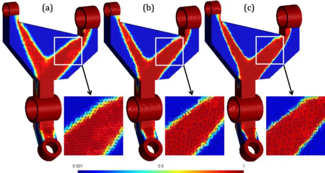
7 shows that this new neighbourhood solves the inconsistency in filtering sensitivity and density. Table 2 also shows that the final compliance always decreases along successive SIMP optimizations and that it converges, after two mesh adaptations to 10,25 Joules (compared to 13,25 Joules). If compared to the results obtained with a constant size mesh in Figure 1b, although the optimal topologies are similar, the quality in the definition of the optimal shape boundary is significantly improved after two levels of mesh adaptation. This adaptation enables a better distribution of the normalized material density at the solid-void interface, which thereby increases accuracy in the description of the optimal shape boundary. Results obtained are similar to those presented in [23, 37] for 2D cases and without de-refinement. The CPU time is related to computational cost of FEA and optimization iterations. As shown in the table, less CPU time is required after the first mesh adaptation, despite a higher number of SIMP iterations. Indeed,
15 thanks to mesh de-refinement, the mesh features substantially less elements than the initial uniform mesh. More CPU time is required after the second mesh adaptation because this adaptation essentially induces mesh refinement and because the convergence criterion ∆𝑐𝑜𝑛𝑣2 =
0,32 % is lower compared to ∆𝑐𝑜𝑛𝑣1 = 0,8 %.
Number of
iterations Optimization time (s)
SIMP convergence criterion (%) Compliance (Joules) Initial mesh 11 287 2,00 12,18 1st adaptation 17 151 0,80 10,75 2nd adaptation 36 390 0,32 10,25 Total 64 828
Table 2 : Adaptive topology optimization data results after three SIMP processes and two mesh adaptations for the bike suspension rocker shown in Figure 7.
Figure 7 : Relative density distribution at the end of SIMP iterations obtained (a) using a
uniform and relatively coarse mesh (with 𝑑𝑔 = 3,5 𝑚𝑚) (b) and (c) after the first and second
mesh adaptations with µ = 9.
3.2.6 Effect of mesh adaptation on mesh quality
Our meshes are made with 3D unstructured tetrahedral elements, and the numerous FEA calculations involved in SIMP optimization are very sensitive to mesh quality. Automatic mesh generation and adaptation is based on the advancing front method [32, 41]. The quality of tetrahedrons is classically measured using [41]:
16 𝑄𝑒 = 𝛼 ∙ 𝑟𝑖𝑛𝑠
𝑙𝑚𝑎𝑥
Where 𝑙𝑚𝑎𝑥 is the longest element edge and 𝑟𝑖𝑛𝑠 the radius of the inscribed sphere. Taking 𝛼 =
2. √6 makes that 𝑄𝑒 = 1 for an equilateral element and 0 for degenerate elements. Figure 8
illustrates meshes used to carry out the three optimizations introduced in Figure 7 and statistics about mesh quality in terms of elements shape and the respect of the sizing function are given in Table 3.
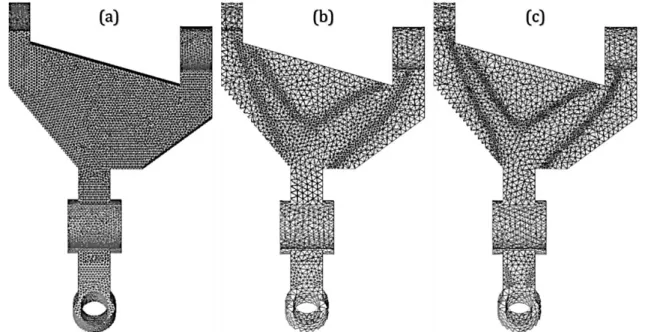
Figure 8 : Meshes used in SIMP results presented in Figure 7 (a) the initial uniform mesh (b) and (c) meshes after the first and second adaptations.
Number of tetrahedra Errorglobal
(%) % elements quality predicted actual 𝑸𝒆≤0,1 0,1<𝑸𝒆≤ 0,2 0,2<𝑸𝒆≤ 0,5 𝑸𝒆> 0,5 Initial mesh 201 398 169 962 15,61 0,02 0,04 19,88 80,06 1st adaptation 90 350 75 051 16,93 0,05 0,11 27,71 72,13 2nd adaptation 130 973 100 028 23,63 0,05 0,08 29,73 70,13 Table 3 : Respect of the size map and mesh quality associated with Figure 8.
It shows that the percentage of very good quality elements decreases from 80% to 70% with mesh adaptation while the number of bad quality elements slightly increases. Mesh quality could be further improved by applying mesh transformation techniques but, since the design domain is entirely re-meshed at each adaptation, the expected gain on mesh quality is marginal. However, the effect of applying mesh quality improvement methods could be investigated in future work. Another potential improvement of the adaptive approach proposed in this paper when setting up sizing functions 𝑑𝑗(𝑥, 𝑦, 𝑧) is limiting the gradient 𝑔𝑟𝑎𝑑⃗⃗⃗⃗⃗⃗⃗⃗⃗⃗ (𝑑𝑗). In fact, if sizing functions feature
17 substantial negative effects on the quality of FEA solutions involved in the optimization process and indirectly on the quality of the optimization process itself.
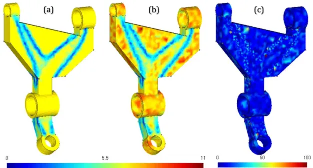
Figure 9 provides a better illustration of the ability of our mesh generation algorithms to respect the imposed sizing function along the mesh adaptation process. Figure 9a shows the prescribed sizing function associated with the second mesh adaptation in Figure 8, while Figure 9b shows the actual distribution of element size after re-meshing. The relative difference between these two distributions (in %) is shown in Figure 9c. The actual minimum and maximum values for mesh sizes are 0,79 𝑚𝑚 − 10,7 𝑚𝑚 , while targeted minimum and maximum sizes were 0,71 𝑚𝑚 − 7 𝑚𝑚. That is due to unavoidable small deviations in the respect of the prescribed size map during automatic mesh generation. In fact, as illustrated in Figure 9c, the imposed sizing function is globally well respected and the deviations are limited and quite local.
Figure 9 : Illustration of the (a) imposed size distribution (b) actual size distribution (c) relative error (in %) after the second adaptation in Figure 8.
3.3 Effect of µ and initial mesh size on optimization results
The previous section introduced our new adaptive topology optimization scheme. In this section, we illustrate the effect, on the process, of two main parameters of the approach. These parameters are µ and the initial mesh size.
3.3.1 Effect of µ
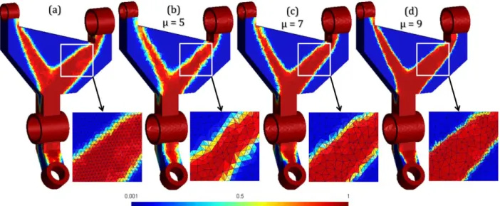
In this sub-section, we investigate the effect of parameter µ on the mesh adaptation process. We perform the adaptive SIMP optimization on the same example as in Figure 7 with different values of µ. Figure 10 shows the solution obtained with an initial uniform mesh size 𝑑𝑔 =
3,5 𝑚𝑚 (Figure 10a) and results, after two levels of adaptation, for µ = 5 (Figure 10b), µ = 7 (Figure 10c) and µ = 9 (Figure 10d). In all cases, 𝐸𝑛𝑚 = 7 𝑚𝑚, which means that the maximum
18 when µ increases, which makes that boundaries between solid and void are better defined. As a matter of fact, when µ = 5, the minimum size (3,52 𝑚𝑚) is almost equal to the initial uniform size (3,5 𝑚𝑚) and nearly only de-refinement is applied. For comparison, when µ = 7 and µ = 9, the mesh is simultaneously refined and de-refined (minimum and maximum sizes are respectively 1,41 𝑚𝑚 − 7 𝑚𝑚 and 0,71 𝑚𝑚 − 7 𝑚𝑚).
Figure 10 : Effect of parameter µ. Relative density distribution at the end of SIMP iterations
obtained (a) using a uniform and relatively coarse mesh with 𝑑𝑔 = 3,5 𝑚𝑚, (b), (c) and (d) after
two mesh adaptations with µ = 5, µ = 7 and µ = 9.
3.3.2 Effect of the initial mesh size
In Figure 11 we illustrate results obtained when solving the same optimization problem as in Figure 7 but starting with a coarser constant size mesh (𝑑𝑔 = 5,0 𝑚𝑚 if compared to 𝑑𝑔 =
3,5 𝑚𝑚 for Figure 7). Minimum and maximum mesh sizes are 2,48 𝑚𝑚 − 7 𝑚𝑚 for the first mesh adaptation (Figure 11b), 1,36 𝑚𝑚 − 7 𝑚𝑚 for the second (Figure 11c) and 0,71 𝑚𝑚 − 7 𝑚𝑚 for the third (Figure 11d). For the same values of µ and 𝐸𝑛𝑚, three steps of mesh adaptation (instead of 2 steps for 𝑑𝑔 = 3,5 𝑚𝑚 in Figure 7) were necessary to obtain similar
optimum mesh sizes. As expected (see
Table 4), the finer the initial mesh size, the lower the final compliance (10,57 Joules for 𝑑𝑔 =
19
Number of
iterations Optimization time (s)
SIMP convergence criterion (%) Compliance (Joules) Initial mesh 12 99 2,000 13,43 1st adaptation 19 221 0,800 12,08 2nd adaptation 37 503 0,320 11,10 3rd adaptation 32 804 0,128 10,57 Total 100 1627
Table 4 : Adaptive topology optimization data results after four SIMP processes and three mesh adaptations for the bike suspension rocker shown in Figure 11.
Figure 11 : Effect of the initial mesh size. Relative density distribution at the end of SIMP
iterations obtained (a) using a uniform and coarser mesh with 𝑑𝑔 = 5,0 𝑚𝑚, (b), (c) and (d)
after the first, second and third mesh adaptations with µ = 9.
In Figure 12 we present a comparison between final SIMP results and optimal shapes derived for the cases in Figure 7 and Figure 11. Figure 12a and Figure 12d present SIMP results, and rough optimal shapes presented in Figure 12b and Figure 12e are obtained from it using 𝜌𝑡ℎ = 0,45.
These rough optimal shapes are processed as explained in [42] (removal of non-manifold patterns followed by mesh smoothing), which leads to the final optimal shapes illustrated in Figure 12c and Figure 12f. It is worth mentioning that mesh smoothing is based on the algorithm presented in [43]. From these optimization results, it appears that changing the initial mesh size leads to quite significant differences in the final result.
20
Figure 12 : Comparison between optimization results obtained in Figure 7 and Figure 11. (a) and (d) Relative density distribution at the end of SIMP iterations (b) and (e) rough optimal
shapes (c) and (f) optimal shapes after smoothing.
4 Results and discussions
The effectiveness of the adaptive TO process presented in the previous sections is demonstrated through the optimization of the 3D models of two mechanical parts (a connecting rod and a cantilever beam). In these two examples, Young’s modulus is 69 GPa and Poisson’s ratio is 0,33.
21 4.1 First example: connecting rod
The next example presented is the adaptive optimization of a connecting rod. Figure 13a introduces the initial geometry of the connecting rod with BCs and loads applied. The initial connecting rod overall dimensions are 350 𝑚𝑚 (height), 150 𝑚𝑚 (width) and 25 𝑚𝑚 (thickness). Null displacements are imposed on the lower-half of the lower bore, and the load is applied (in the 𝑌 direction) on the upper-half of the upper bore. As seen in the SIMP result presented in Figure 13b, non-design material is distributed around the two connecting bores. This result is based on an initial uniform relatively coarse mesh (with 𝑑𝑔 = 4,5 𝑚𝑚) without adaptive
refinement and the volume fraction imposed is 𝑓 = 0,3. The norm of relative density gradient derived from the SIMP result is presented in Figure 13c. In Figure 14, we introduce mesh adaptation on the same case as in Figure 13. Figure 14a illustrates a 2D view of the result obtained in Figure 13b with the initial uniform mesh (with 𝑑𝑔 = 4,5 𝑚𝑚). Then, Figure 14b,
Figure 14c and Figure 14d show the effects of three successive mesh adaptations on SIMP results obtained. This adaptation considers 𝐸𝑛𝑚 = 9 𝑚𝑚 and µ = 11. Minimum element sizes
are 2,40 𝑚𝑚, 0,65 𝑚𝑚 and 0,30 𝑚𝑚 respectively after the first, second and third mesh adaptation. From Figure 14 and
Table 5, it is clear that higher resolution of the structural boundaries and better compliances are achieved along mesh adaptations.
Figure 13 : connecting rod (a) model, loads and boundary conditions, (b) relative density
distribution at the end of SIMP iterations using a uniform mesh (𝑑𝑔 = 4,5 𝑚𝑚) and (c) relative
22
Figure 14 : Relative density distribution at the end of SIMP iterations obtained on the
connecting rod (a) using a uniform and relatively coarse mesh (with 𝑑𝑔 = 4,5 𝑚𝑚), (b), (c) and
(d) after the first, second and third mesh adaptations with µ = 11.
Number of
iterations Optimization time (s)
SIMP convergence criterion (%) Compliance (Joules) Initial mesh 11 160 1,000 0,051 1st adaptation 14 59 0,100 0,043 2nd adaptation 18 100 0,010 0,042 3rd adaptation 22 206 0,001 0,042 Total 65 525
Table 5 : Adaptive topology optimization data results after four SIMP processes and three mesh adaptations for the connecting rod shown in Figure 14.
Figure 15 shows the initial uniform mesh and the meshes obtained after the different steps of adaptation. Associated statistics about mesh quality and respect of the prescribed size map are summarized in Table 6. Like in the case of the bike suspension rocker, percentage of good-quality elements decreases from 82% to 61,5% along mesh adaptation. The actual minimum and maximum values for mesh sizes are 0,285 𝑚𝑚 − 12,5 𝑚𝑚, if compared to the imposed values which are 0,3 𝑚𝑚 − 9,0 𝑚𝑚.
23
Figure 15 : Meshes used in SIMP results presented in Figure 14 (a) the initial uniform mesh (b),(c) and (d) meshes after the first, second and third adaptations.
Number of tetrahedra Errorglobal
(%) % elements quality predicted actual 𝑸𝒆≤0,1 0,1<𝑸𝒆≤ 0,2 0,2<𝑸𝒆≤ 0,5 𝑸𝒆> 0,5 Initial mesh 126 744 114 544 9,63 0,00 0,03 18,03 81,94 1st adaptation 36 006 33 014 8,31 0,05 0,06 27,52 72,37 2nd adaptation 52 804 45 524 13,79 0,03 0,11 31,45 68,40 3rd adaptation 150 441 100 720 33,05 0,03 0,13 38,42 61,42 Table 6 : Respect of the size map and mesh quality associated with Figure 15.
The optimal shape, as shown in Figure 16, is obtained using 𝜌𝑡ℎ = 0,45 and the same
post-processing operations are applied as for the example shown in Figure 12. It demonstrates the ability of the proposed approach to generate symmetrical designs with high-quality boundary description using asymmetric and unstructured tetrahedral meshes.
24
Figure 16 : Connecting rod (a) final relative density distribution at the end of SIMP iterations after 3 steps of adaptation with µ = 11 (b) rough optimal shape and (c) optimal shape after
smoothing.
4.2 Second example: cantilever beam
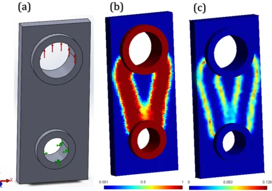
The second example considered is the optimization of a cantilever beam, which is a case that has been studied (mostly in 2D) by several authors [18, 20, 23, 25, 26, 37]. The initial beam features a square cross-section (50 𝑚𝑚 × 50 𝑚𝑚) and length 𝐿 = 250 𝑚𝑚. It is anchored at one end and loaded at the other end in the 𝑌 direction (see Figure 17a). As seen in the SIMP result presented in Figure 17b, non-design material is distributed around the anchor surface and around the load. In this case, the volume fraction is 𝑓 = 0,4. The solution obtained and the corresponding relative density gradient are shown respectively in Figure 17b and Figure 17c. This result is obtained with a uniform and relatively coarse mesh with 𝑑𝑔 = 4 𝑚𝑚.
In Figure 18, we introduce mesh adaptation on this same case along with the details of material and void distributions inside the beam section (using a cutting plane for each case). Figure 18a illustrates two views of the result obtained in Figure 17b with the initial uniform mesh (with 𝑑𝑔 = 4 𝑚𝑚). Then, Figure 18b and Figure 18c show the effects of two successive mesh
adaptations on SIMP results obtained. This adaptation considers 𝐸𝑛𝑚 = 5 𝑚𝑚 and µ = 7. The
compliance finally converges to 0,063 Joules with a final convergence criterion ∆𝑐𝑜𝑛𝑣2 = 0,01 %
after 41 iterations (see Table 7).
25
Figure 17 : Cantilever beam (a) model, loads and boundary conditions, (b) relative density
distribution at the end of SIMP iterations using a uniform mesh size (𝑑𝑔 = 4 𝑚𝑚) and (c)
relative density gradient derived : high values (light-blue and yellow) and zero gradient (dark-blue).
Number of
iterations Optimization time (s)
SIMP convergence criterion (%) Compliance (Joules) Initial mesh 12 122 1,000 0,079 1st adaptation 14 216 0,100 0,068 2nd adaptation 15 338 0,010 0,063 Total 41 676
Table 7 : Adaptive topology optimization data results after three SIMP processes and two mesh adaptations for the cantilever beam shown in Figure 18.
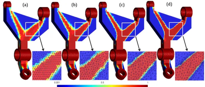
The same trend as in the previous examples can be seen: the mesh adaptation significantly refines the definition of the optimal shape boundary.
26
Figure 18 : Relative density distribution at the end of SIMP iterations obtained on the cantilever
beam (a) using a uniform and relatively coarse mesh (with 𝑑𝑔 = 4 𝑚𝑚) (b) and (c) after the first
and second mesh adaptations with µ = 7.
Figure 19 shows the initial uniform mesh and the meshes obtained after the different steps of mesh adaptation. Associated statistics about mesh quality and the respect of the prescribed size map are summarized in Table 8.
Figure 19 : Meshes used in SIMP results presented in Figure 18 (a) the uniform mesh (b) and (c) meshes after the first and second adaptations.
27
Number of tetrahedra Error(%) global % elements quality
predicted actual 𝑸𝒆≤0,1 0,1<𝑸𝒆≤ 0,2 0,2<𝑸𝒆≤ 0,5 𝑸𝒆> 0,5
Initial mesh 82 914 70 663 14,78 0,00 0,01 17,67 82,31
1st level 133 511 102 608 23,15 0,00 0,03 24,67 75,30
2nd level 212 306 148 708 29,96 0,00 0,02 25,90 74,09 Table 8 : Respect of the size map and mesh quality associated with Figure 19.
The optimal shape obtained is shown in Figure 20. It is also obtained using 𝜌𝑡ℎ = 0,45 and the
same post-processing operations are applied as for the examples shown in Figure 12 and Figure 16. This example is interesting, if compared to the previous ones, because material distribution moves to the boundaries of the initial volume along the adaptive SIMP optimization process. Indeed, as illustrated in Figure 18, material is concentrated around the square section and the interior volume is empty.
Figure 20 : Cantilever beam (a) final relative density distribution at the end of SIMP iterations after 2 steps of adaptation with µ = 7 (b) rough optimal shape (c) optimal shape after
smoothing.
A closer look at the evolution of a cross section along the adaptive optimization process provides a good illustration and understanding of what happens. Figure 21 shows cross sections of the SIMP relative density and of the associated norm of gradient, for the uniform mesh (Figure 21a) and for the 2 steps of adaptive refinement and de-refinement (Figure 21b and Figure 21c)
28 illustrated in Figure 18. It clearly demonstrates that, in a given section along the beam, the optimization process increases upper and lower wall thicknesses while it decreases right and left wall thicknesses. This is consistent with the fact that the bending strength of the cantilever beam globally increases with the moment of inertia of the beam section. Theoretically, as illustrated in Figure 22 and as addressed by [44], with a given amount of material, the optimal moment of inertia corresponds to thickening to the maximum the upper and lower flanges (thickness ℎ) and decreasing the vertical thickness 𝑤 so that it tends to zero. The results shown in Figure 21 demonstrate that our adaptive optimization process converges to a square hollow section as in Figure 22a. Standard sections based on a I profile (like in Figure 22b) are better, in this context, because the equivalent thickness 𝑤 of the vertical web is twice the wall thickness ( 𝑤
2 ) of the
equivalent square hollow section Figure 22a. Both sections feature the same moment of inertia 𝐼𝑥𝑥 but the minimum web thickness is limited by localized buckling in the web. Of course, the SIMP method, as implemented in this work, is based on linear mechanics, which means that local buckling is not taken into account in the optimization process. In this context, these two sections are equivalent and it is consistent that the process converges to a square hollow section. It also appears that, with the adaptive SIMP optimization process, if we used a more refined mesh, the result would tend to get closer to the optimal section, which means tend to increase wall thickness ℎ and decrease wall thickness 𝑤
2.
Figure 21 : Evolution of the internal solid-void interface after (a) the first, (b) the second, and (c) the third SIMP process. Upper figures show relative density distributions at the end of each
SIMP and lower figures show the relative density gradient derived : high values (yellow and orange) and zero gradient (dark-blue).
29
Figure 22 : (a) A square hollow cross-section (b) An equivalent I-profile cross-section.
5 Conclusion
In this paper, a new adaptive topology optimization method is presented for the optimization of continuum structures. The aim of this work is to converge towards higher resolution in the definition of optimal shapes obtained after optimization, but at a reasonable computational cost. This method is based on an implementation of the SIMP method that handles 3D optimization problems by using unstructured tetrahedral meshes. The mesh adaptation scheme proposed is fully automatic and it is based on the SIMP relative density gradient. The scheme features simultaneous mesh refinement and de-refinement. An important conclusion is that this adaptive process requires revisiting classical sensitivity and density filtering schemes. Even if the approach is very promising and applicable to other TO schemes, several enhancements of the method can easily be foreseen. Actually, it has been mentioned that no explicit limitation is put on the gradient of mesh sizing functions, which contributes to undermine mesh quality, and by the way, the quality of the optimization itself. We have seen that sensitivity and relative density filtering are very sensitive to mesh refinement. This suggests that the extension of classical filtering techniques, in the context of using adaptive meshes with steep mesh size variations, should be studied thoroughly. Moreover, our approach introduces several new parameters, which adds to numerous parameters that are associated with the SIMP method itself. Studying the influence of these parameters on optimization results is also a source of potential future work on the subject. Last but not least, the automatic (or at least assisted) creation of CAD models from optimization results is also clearly a natural perspective for further research work on the subject. This objective represents an important source of research interest but it is also an extremely complex and ambitious problem because building a good optimal shape from TO results is subject to numerous constraints (shape, mass, strength, vibrations, manufacturing, etc.) that, in many cases, are partly (or even completely) contradictory.
6 Acknowledgement
This study was carried out as part of a project supported by the Natural Sciences and Engineering Research Council of Canada (NSERC) and UQTR foundation.
30 7 References
1. Bendsoe, M.P. and O. Sigmund, Topology optimization - Theory,Methods and
Applications. 2nd ed. 2003, Berlin: Springer. 370.
2. Deaton, J.D. and R.V. Grandhi, A survey of structural and multidisciplinary continuum
topology optimization: Post 2000. Structural and Multidisciplinary Optimization, 2014.
49(1): p. 1-38.
3. Jang, G.-W., K.J. Kim, and Y.Y. Kim, Integrated topology and shape optimization
software for compliant MEMS mechanism design. Advances in Engineering Software,
2008. 39(1): p. 1-14.
4. Cugini, U., et al., Integrated Computer-Aided Innovation : The PROSIT approach. Computers in Industry, 2009. 60: p. 629-641.
5. Zhou, M., et al., Topology Optimization - Practical Aspects for Industrial Applications. Proceedings of the 9th World Congress on Structural and Multidisciplinary Optimization, June 13 - 17, Shizuoka, Japan, 2011.
6. Bendsøe, M.P., Optimal shape design as a material distribution problem. Structural Optimization, 1989. 1(4): p. 193-202.
7. Suzuki, K. and N. Kikuchi, A homogenization method for shape and topology
optimization. Computer Methods in Applied Mechanics and Engineering, 1991. 93(3): p.
291-318.
8. Allaire, G., Z. Belhachmi, and F. Jouve, The homogenization method for topology and
shape optimization. Single and multiple loads case. Revue Europeenne des Elements,
1996. 5(5-6): p. 649-672.
9. Wang, M.Y., X. Wang, and D. Guo, A level set method for structural topology
optimization. Computer Methods in Applied Mechanics and Engineering, 2003. 192(1-2):
p. 227-246.
10. Yulin, M. and W. Xiaoming, A level set method for structural topology optimization and
its applications. Advances in Engineering Software, 2004. 35(7): p. 415-441.
11. Querin, O.M., G.P. Steven, and Y.M. Xie, Evolutionary structural optimisation (ESO)
using a bidirectional algorithm. Engineering Computations (Swansea, Wales), 1998.
15(8): p. 1031-1048.
12. Zuo, Z.H. and Y.M. Xie, A simple and compact Python code for complex 3D topology
optimization. Advances in Engineering Software, 2015. 85: p. 1-11.
13. Aremu, A., et al. Suitability of SIMP and BESO topology optimization algorithms for
additive manufacture. in 21st Annual International Solid Freeform Fabrication Symposium - An Additive Manufacturing Conference, SFF 2010. 2010.
14. Brackett, D., I. Ashcroft, and R. Hague. Topology optimization for additive
manufacturing. in 22nd Annual International Solid Freeform Fabrication Symposium - An Additive Manufacturing Conference, SFF 2011. 2011.
15. Maute, K. and E. Ramm, Adaptive topology optimization. Structural Optimization, 1995. 10(2): p. 100-112.
16. Ramm, E., K. Maute, and S. Schwarz, Adaptive topology and shape optimization. Computational Mechanics, New Trends and Applications, Barcelona, Spain, 1998.
17. Arantes Costa Jr, J.C. and M.K. Alves, Layout optimization with h-adaptivity of
structures. International Journal for Numerical Methods in Engineering, 2003. 58(1): p.