HAL Id: hal-02390212
https://hal.archives-ouvertes.fr/hal-02390212
Submitted on 26 Mar 2020
HAL is a multi-disciplinary open access
archive for the deposit and dissemination of
sci-entific research documents, whether they are
pub-lished or not. The documents may come from
teaching and research institutions in France or
abroad, or from public or private research centers.
L’archive ouverte pluridisciplinaire HAL, est
destinée au dépôt et à la diffusion de documents
scientifiques de niveau recherche, publiés ou non,
émanant des établissements d’enseignement et de
recherche français ou étrangers, des laboratoires
publics ou privés.
A simplified and versatile calibration method for
multi-camera optical systems in 3D particle imaging
Nathanaël Machicoane, A. Aliseda, R. Volk, Mickaël Bourgoin
To cite this version:
Nathanaël Machicoane, A. Aliseda, R. Volk, Mickaël Bourgoin. A simplified and versatile calibration
method for multi-camera optical systems in 3D particle imaging. Review of Scientific Instruments,
American Institute of Physics, 2019, 90 (3), pp.035112. �10.1063/1.5080743�. �hal-02390212�
3D particle imaging
Cite as: Rev. Sci. Instrum. 90, 035112 (2019); https://doi.org/10.1063/1.5080743
Submitted: 11 November 2018 . Accepted: 28 February 2019 . Published Online: 22 March 2019 N. Machicoane , A. Aliseda , R. Volk, and M. Bourgoin
ARTICLES YOU MAY BE INTERESTED IN
Denoising of surface electromyogram based on complementary ensemble empirical mode
decomposition and improved interval thresholding
Review of Scientific Instruments
90, 035003 (2019);
https://doi.org/10.1063/1.5057725
New light trap design for stray light reduction for a polarized scanning nephelometer
Review of Scientific Instruments
90, 035113 (2019);
https://doi.org/10.1063/1.5055672
A high speed X-Y nanopositioner with integrated optical motion sensing
Review of
Scientific Instruments
ARTICLE scitation.org/journal/rsiA simplified and versatile calibration method
for multi-camera optical systems in 3D
particle imaging
Cite as: Rev. Sci. Instrum. 90, 035112 (2019);doi: 10.1063/1.5080743
Submitted: 11 November 2018 • Accepted: 28 February 2019 • Published Online: 22 March 2019
N. Machicoane,1,a) A. Aliseda,1 R. Volk,2 and M. Bourgoin2 AFFILIATIONS
1Department of Mechanical Engineering, University of Washington, Seattle, Washington 98195, USA
2University of Lyon, ENS de Lyon, Université Claude Bernard, CNRS, Laboratoire de Physique, F-69342 Lyon, France
a)Electronic mail:[email protected]
ABSTRACT
This article describes a stereoscopic multi-camera calibration method that does not require any optical model. It is based on a measure of the light propagation within the measurement volume only instead of modeling its entire path up to the sensors. The calibration uses simple plane by plane transformations which allow us to directly link pixel coordinates to light rays. The appeal of the proposed method relies on the combination of its simplicity of implementation (it is particularly easy to apply in any sophisticated optical imaging setup), its versatility (it can easily handle index-of-refraction gradients, as well as complex optical arrangements), and its accuracy {we show that the proposed method gives better accuracy than commonly used techniques, based on Tsai’s simple pinhole camera model [R. Tsai, J. Rob. Autom. 3, 323 (1987)], while its numerical implementation remains extremely simple}. Based on ideas that have been available in the fluid mechanics community, this method is a compact turn-key algorithm that can be implemented with open-source routines.
Published under license by AIP Publishing.https://doi.org/10.1063/1.5080743
I. INTRODUCTION
Flow velocity measurements, based on the analysis of the motion of particles imaged with digital cameras, have become the most commonly used metrology technique in contemporary fluid mechanics research.1,2Particle Image Velocimetry (PIV) and Parti-cle Tracking Velocimetry (PTV) are two widely used methods that enable the characterization of a flow from an Eulerian (PIV) or Lagrangian (PTV) point of view. Additionally, particle imaging is used in image correlation techniques that provide strain or strain rate measurements,3,4and PTV can yields information about a dis-persed phased carried by the flow.5–8Several aspects influence the accuracy and reliability of the measurements obtained with these techniques:9 resolution (temporal and spatial), dynamical range (spatial and temporal), capacity to measure 2D or 3D components of velocity in a 2D or 3D domain, or statistical convergence. These imaging and analysis considerations depend not only on the hard-ware (camera resolution, repetition rate, on board memory, or optical system) but also on the software (optical calibration, par-ticle identification and tracking algorithms, image correlations, or dynamical post-processing) used in the measurements.
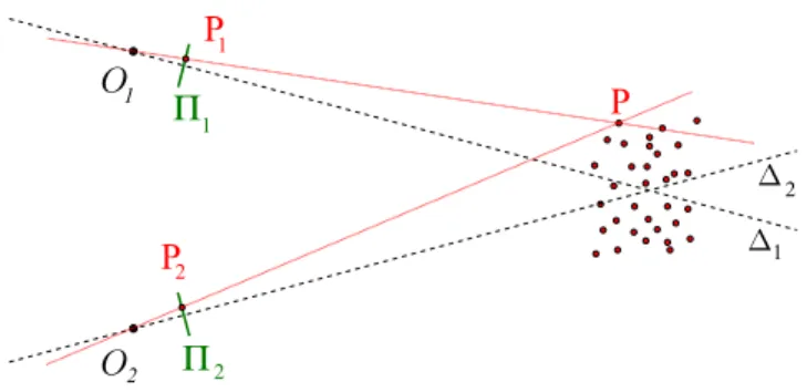
In the context of particle tracking with applications in fluid mechanics, particle center detection and tracking algorithms have been the focus of more studies10,11,22than optical calibration and 3D position determination. Although many strategies with vari-ous degrees of complexity have been developed for camera cali-bration,12–17most existing experimental implementations of multi-camera particle tracking use the pinhole multi-camera model, originally proposed by Tsai in 198718 as the basis for calibration (sketched inFig. 1).13Tsai’s model requires non-linear elements to account for each aspect of the optical path. In practice, realistic experimental setups are either complex or time-consuming to model via individ-ual optical elements in the Tsai method or are over-simplified by ignoring certain elements such as windows or compound lenses, with loss of accuracy.
This article describes a new camera calibration method that can be more accurate than a simple Tsai model in terms of absolute 3D stereo-positioning of particles, while easily handling any of the com-plexity or non-linearity in the optical setup described above. The key point of the method is that, instead of defining an optical model of the imaging system, it defines, without any physical a priori model, a transformation that connects each point in the camera sensor to
Rev. Sci. Instrum. 90, 035112 (2019); doi: 10.1063/1.5080743 90, 035112-1
FIG. 1. Sketch of Tsai’s pinhole camera model and stereo-matching: the position
of a particle in the real world corresponds to the intersection of 2 lines∆1and∆2,
each emitted by the camera centers O1and O2and passing through the position
of particles P1and P2detected on a each camera planeΠ1andΠ2.
the actual light beam across the measurement volume. This trans-formation contains the necessary degrees of freedom but does not require any operator input beyond a set of calibration images taken across the measurement volume (typical of any 3D calibration pro-cess). The multi-camera calibration proposed can be applied to other 3D imaging setups such as tomographic PIV or PTV.
II. CALIBRATION PRINCIPLE
3D particle imaging methods require an appropriate calibration method to perform the stereo-matching between the several sets of 2D positions of particles in the pixel coordinate system for each cam-era and the absolute 3D position of the particles in the real-world coordinate system. The accuracy of the calibration method directly impacts the accuracy of the 3D positioning of the particles in the real world.
The calibration method proposed here is based on the sim-ple idea that no matter how distorted a recorded image is, each bright point on the pixel array is associated with the ray of light that produced it, such that the corresponding light source (typically a scattering particle) can lie anywhere on this ray of light. An appro-priate calibration method should be able to directly attribute to a given doublet (xp, yp) of pixel coordinates the corresponding ray
path. If the index of refraction in the measurement volume of inter-est is uniform (so that light propagates along a straight line inside the measurement volume), each doublet can be associated with a straight line ∆ (defined by 6 parameters in 3D: one point O∆and
one vector ⃗V∆), regardless of the path outside the volume of
inter-est, which can be very complex as material interfaces and lenses are traversed. The method consists in building a pixel-to-line transfor-mation I to perform this correspondence between pixel coordinates and each of the 6 parameters of the ray of light: (xp, yp)
I
Ð→ (O∆, ⃗V∆).
Note that in the experimental demonstration of the methods pro-posed here, it is assumed that light propagates in a straight line as the medium in the experiment presented is homogeneous, but, as dis-cussed below, it is trivial to extend the method to handle curved light path.
While the proposed method can seem similar to the Tsai approach, since it also builds a ray of light for each doublet, there is a significant difference in that Tsai’s approach which assumes a physical model for the camera and optical path, with few parameters
The quality of the inferred transformation will therefore be sensi-tive to variations of the setup leading to calibration data which may no longer match the model due to optical distortions, imperfect interfaces, sophisticated optical arrangements (such as a tilt-and-shift lens), and other possible complexities. Handling such complex-ities in pinhole-like models is doable but generally requires specific modifications of the underlying model (implying generally complex algorithms, difficult at least for non-experts). The present approach, based on empirical transformations from the actual calibration data, embeds an arbitrary number (as described below) of parameters that are not related to any physical property of the optical system. The calibration, therefore, self-adapts to optical imperfections, media inhomogeneities (outside of the measurement volume), or complex lens arrangements. Additionally, the generalization of the method to cases where light does not propagate in a straight line is straightfor-ward: it is sufficient to build the transformation I with the param-eters required to describe the expected curved path of light in the medium of interest (for instance, a parabola in a linearly stratified medium or an arbitrary higher order polynomial for more complex situations).
III. PRACTICAL IMPLEMENTATION
An implementation of the method is proposed where the pixel-to-line transformation I is built as an interpolant from experimental images of a calibration target with known patterns at known posi-tions. The open-source routines described below are provided in the
supplementary material. The process is described for one camera only for clarity’s sake.
A calibration target consisting in a grid of equally separated dots is moved perpendicularly to its plane (along the OZ axis) using a micrometric screw, being imaged at several known Z positions by all cameras. Note that micrometric translation of planes is not a priori required, and a set of images of points with known location, in arbi-trary planes, can very well be used instead. Also, with minor changes, other planar patterns than points (such as a checkboard pattern) can also be used. In total, NZ plane images are taken with each
camera: Ijis the calibration image when the plane is at position Zj
(with j ∈ [1, NZ]). For the purpose of testing, the quality of the
cal-ibration method and its sensitivity to the number of planes used, up to NZ= 13 planes, were collected across the measurement
vol-ume. The calibration protocol, sketched inFig. 2, then proceeds as follows:
1. Dot center finding. For each calibration image Ij, the dot
centers are detected, giving a set (xkj, ykj)k∈[1;Nj]of pixel
coor-dinates. Nj is the number of dots actually detected on each
image Ij. Real-world coordinates of the dots (Xjk, Yjk, Zkj)k∈[1;Nj]
are known. Lowercase coordinates represent pixel coordinates, while uppercase coordinates represent absolute real-world coordinates.
2. 2D plane-by-plane transformations. For each position Zj
of the calibration target, the measured 2D pixel coordi-nates (xkj, ykj)k∈[1;N
j]and the known 2D real-world coordinates
(Xkj, Yjk)k∈[1;Nj] are used to infer a spatial transformation Tj
projecting 2D pixel coordinates onto 2D real-world coordi-nates in the plane XOY at position Zj. Different types of
Review of
Scientific Instruments
ARTICLE scitation.org/journal/rsiFIG. 2. Sketch of the calibration method. (a) Calibration target imaged on one plane, over Nx×Nypixels. (b) Same plane transformed into real-world coordinates on the
domain LX×LY(no optical distortion is considered here for simplicity so the transformation is linear in the 2D plane). (c) Stacks of planes in 3D real-world coordinates. Dots
at (X, Y) are fitted along Zi, 1 ≤ i ≤ NZto build the interpolantI. For simplicity, only 3 planes are considered here with the 3 dots identified as crosses and a linear fit is used
(dashed line). Note that the fit is only done within the calibration volume where the target is translated along the Nzplanes and does not extend to the cameras.
transformations can be inferred from a simple linear projec-tive transformation to high order polynomial transformations if non-linear optical aberrations need to be corrected (com-mon optical aberrations are adequately captured by a 3rd order polynomial transformation). This is a standard planar calibration procedure, where an estimate of the accuracy of the 2D plane-by-plane transformation can be obtained from the distance, in pixel coordinates, between (xkj, ykj)k∈[1;Nj]and Tj−1(Xjk, Yjk, Zj)
k∈[1;Nj]. The maximum error for the images
used here is less than 2 pixels.
3. Building the pixel-line interpolant. The key step in the cal-ibration method builds the pixel-line interpolant, I, which directly connects pixels coordinates to a ray path. To achieve this, a grid of NI interpolating points in pixel coordinates
(xlI, ylI)l∈[1,N
I]is defined, for which the ray paths have to be
computed. The inverse transformations Tj−1are used to project
each point of this set back onto the real-world planes (X, Y, Zj), for each of the NZpositions Zj. Each interpolating point
(xlI, ylI)is therefore associated with a set of NZpoints in the real world (XIl, YlI, Zj). Conversely, these points in the real
world can be seen as a discrete sampling of the ray path which impacts the sensor of the camera at (xIl, y
I
l). If light
propa-gates as a straight line, the NZpoints (XlI, YlI, Zj)should be aligned. By a simple linear fit of these points, each interpo-lating point (xIl, yIl)is related to a line ∆l, defined by a point O∆l = (X 0 l, Y 0 l, Z 0
l)and a vector ⃗V∆l = (Vxl, Vyl, Vzl)(hence
6 parameters for each interpolating point). Each of these rays from the NIinterpolation points is used to compute the
inter-polant I, which allows any pixel coordinate (x, y) in the camera to be connected to its ray path (O∆, ⃗V∆)corresponding to all possible positions of light sources that could produce a bright spot in (x, y). Finding the 3D position of a point (or particle) can be done by finding the location of crossing of all the rays coming from the different cameras. All pixels in each camera were chosen here to build the interpolant as this step is done only once, but the method can be applied with a sub-sampled
pixel array. Alternatively, one can also choose not to build the interpolant but to apply the plane-by-plane transformations and the polynomial fit leading to the light ray directly from the actual data (for instance, corresponding to detected centers of particle images).
IV. COMPARISON WITH THE TSAI METHOD
The calibration procedure proposed by Tsai18has been widely used to recover the optical characteristics of an imaging system and reconstruct the 3D position of an object. The accuracy of the pro-posed imaging calibration procedure is assessed by comparing it with a simple Tsai implementation. Given the simplicity of imple-mentation of the proposed method, we consider for the present com-parison a simple version of the Tsai model, accounting only for cubic radial distortion. While improved optical elements modeling in the Tsai model could increase the accuracy, they come at an increased user workload.
The stereoscopic optical arrangement is sketched inFig. 3. It aims at performing particle tracking velocimetry in a 1 cm-thick laser sheet near the geometrical center of a turbulent water flow cre-ated in an icosahedron [the Lagrangian Exploration Module (LEM) flow; see Refs.19,20, and23for more details]. Each camera objec-tive, nearly perpendicular to its corresponding window, is mounted in the Scheimpflug configuration21 so that all particles present in the laser sheet are nearly in focus independently of their position in the field of view. To perform both calibrations, we used a translu-cent plate mounted parallel to the laser sheet with dots size equal to 2 mm. These points were equally spaced by a distance of 5 mm in both directions, and the thickness of the plate was approximately 0.2 mm. This plate was attached to a manual micro-metric traverse that was able to give displacements with an accuracy of the order of 10 µm. For both methods, up to 13 images of the target were used, spaced 1 mm from each other along the Z axis. The interpolant for the proposed method was built considering a simple line equation for light propagation as light is expected to propagate straight in the homogeneous medium we considered.
Rev. Sci. Instrum. 90, 035112 (2019); doi: 10.1063/1.5080743 90, 035112-3
FIG. 3. Top view of the stereoscopic optical arrangement used for particle tracking
in the LEM flow. Both cameras use an objective with Scheimpflug mount so that all objects in a 10 × 10 × 1 cm3region near the geometrical center are approximately
in focus on the camera sensor. The calibration mask is placed parallel to the laser sheet and moved in the Z direction.
TABLE I. Absolute deviation from the expected position of the targets averaged over space.
dX(µm) dY(µm) dZ(µm) d (µm)
Proposed calibration 32.7 12.6 39.2 59 Tsai model 121 171.1 112.7 266.6
The calibration methods use the 2D positions of the target dots and provide a series of positions that cannot match exactly the 3D real coordinates because, in both methods, the model param-eters are obtained by solving an over-constrained linear system in the least-square sense. The calibration error, i.e., the absolute difference between the (known) real coordinates and the trans-formed ones, is computed to evaluate the calibration accuracy. This error can be estimated along each direction, e.g., dX, or as a norm:
d =√d2
X+ d2Y+ dZ2(Table I).Figure 4plots the total 3D error
aver-aged on the 13 planes used, for both the proposed method and the Tsai model.
ple Tsai one. The error is at least 300% smaller (depending on which component is considered) and is reduced to barely 0.5 pixel. It is important to note that the error map obtained with the Tsai method [Fig. 4(b)] seems to display a large bias along Y that could be due to the use of Scheimpflug mounts, which are typically not included in this Tsai calibration, and to the angle between the cameras and the tank windows. This hypothesis was verified by comparing the two calibration procedures in more conventional conditions (with-out the Scheimpflug mount and in air in order to avoid intermediate interfaces), where they give similar results with very small error. This also points out that, beyond its accuracy and simplicity of implemen-tation, the proposed calibration method is highly versatile and can be used without modification and without loss of accuracy both in simple optical situations and in complex arrangements.
For the present optical arrangement and the new calibration method, the error in the Y positioning is smallest. Indeed, due to the shape of the experiment (an icosahedron), the y axis of the camera sensor is almost aligned with the Y direction so that this coordi-nate is fully redundant between the cameras, while the x axis of each camera sensor forms an angle α ≃ π/3 with the X direction so that the accuracy on X positioning is lower. This directly impacts the accuracy on the Z positioning whose error is almost equal to the X positioning error.
V. DISCUSSION
Up to 13 planes were used to build the operator that yields the camera calibration. While two planes are the minimum required for the method, a larger number of planes imaged provide better accuracy. In this case study, the major sources of optical distortion were Scheimpflug mounts, imperfect lenses, and non-perpendicular interfaces. 7 planes provided an optimal trade-off between high accuracy and simplicity, with an error only 2% larger than with 13 planes, while using 3 planes yields an error 10% larger. If deal-ing with a more complex experiment, e.g., with a refraction index gradient, increasing the number of planes in the calibration would improve the results allowing the calibration operator to accurately capture the curvature of the light rays. On the contrary, for simpler situations (without interfaces and without Scheimpflug mounts), fewer planes would be required to achieve the same level of accu-racy. As a matter of fact, the number of planes used impacts directly the effective number of hidden parameters in the calibration model and largely determine its accuracy. The 3rd order polynomial plane-by-plane transformations used here embed 10 parameters
FIG. 4. Calibration error averaged over Z using the
Review of
Scientific Instruments
ARTICLE scitation.org/journal/rsieach (corresponding to the polynomial coefficients). The total num-ber of effective degrees of freedom for the total calibration using Nz
planes is, then, Np= 10Nz. The simple Tsai model accounts only for
radial distortions and thus typically embeds only on the order of 10 parameters. Taking this higher number of degrees of freedom into account, the improved accuracy of the proposed method compared to the Tsai model is somehow expected (as using 7 planes leads to a calibration model embedding 70 parameters). The present com-parison may, thus, seem unfair to the Tsai model, but the basis for it was similar ease of implementation and not similar number of degrees of freedom. One can consider more sophisticated pinhole camera models, with additional parameters properly accounting for tilt and shift corrections, up to a point where they would match the accuracy reached with the proposed calibration here, but with much more effort from the user in formulating the complex opti-cal model. This is because such extensions of the pinhole approach are based on sophisticated physical and geometrical models, with algorithms which tend to be tedious to implement. A big advan-tage of the present calibration is its versatility and ease of algorithmic implementation, which remains identical (without loss of accuracy), irrespective of the optical path complexity.
The proposed calibration method has several advantages that make it worth implementing in a multi-camera particle imaging setup. First, it requires no model or assumption about the proper-ties of the optical path followed by the light in the different media outside the volume of interest. The method computes a transforma-tion that directly determines the equatransforma-tion for propagatransforma-tion of light in space (within the volume of interest). This ray equation is fully determined by the Nzplane-by-plane transformations. Second, this
method is turnkey for any typical optical system. The implementa-tion of the new method is easily done and can be used retroactively using previous calibration images.
To conclude, the calibration method proposed combines sim-plicity of implementation, versatility of application, and accuracy. The calibration algorithm and the operator calculation to convert pixel locations to physical locations, with minimal errors, are open-source and given in the thesupplementary materialbut can easily be programmed in any language available to experimentalists. The new method is at least equally, and frequently more, accurate than the commonly used Tsai model, and it can be used more easily and in a wider range of optical configurations. As experimental setups get more complicated with more optical and light refraction elements, this method should prove simpler to implement and more accurate than approaches based on camera models.
SUPPLEMENTARY MATERIAL
Thesupplementary materialcontains the calibration algorithm, as well as examples for the plane-by-plane transform, interpolant
computation, and resulting error estimation that can be tested on the user data or with the provided demo data for testing purposes. ACKNOWLEDGMENTS
The authors would like to acknowledge the financial support of the European EUHIT I3project (Contract No. 312778), Labex TEC 21 (Contract No. ANR-11-LABX-0030), PALSE/2013/26, and IDEXLyon (Contract No. ANR-16-IDEX-0005) under the Univer-sity of Lyon auspices.
REFERENCES
1
R. J. Adrian,Annu. Rev. Fluid Mech.23, 261 (1991). 2
Springer Handbook of Experimental Fluid Dynamics, edited by C. Tropea, A. Yarin, and J. F. Foss (Springer-Verlag, Berlin-Heidelberg, 2007).
3
J. C. del Alamo, R. Meili, B. Alonso-Latorre, J. Rodriguez-Rodriguez, A. Aliseda, R. A. Firtel, and J. C. Lasheras,Proc. Natl. Acad. Sci. U. S. A.104(33), 13343–13348 (2007).
4
J. Rodriguez-Rodriguez, C. Marugan-Cruz, A. Aliseda, and J. C. Lasheras,Exp. Therm. Fluid Sci.35, 301–310 (2011).
5
Y. Sato and K. Yamamoto,J. Fluid Mech.175, 183–199 (1987). 6
M. Virant and T. Dracos,Meas. Sci. Technol.8(12), 1539–1552 (1997). 7
G. A. Voth, A. L. Porta, A. Crawford, J. Alexander, and E. Bodenschatz,J. Fluid Mech.469, 121 (2002).
8
F. Toschi and E. Bodenschatz, Annu. Rev. Fluid Mech. 41, 375–404 (2009).
9
Springer Handbook of Experimental Fluid Dynamics, edited by C. Tropea, A. Yarin, and J. Foss (Springer-Verlag, Berlin, 2007), pp. 789–799.
10
N. Ouellette, H. Xu, and E. Bodenschatz,Exp. Fluids40, 301 (2006). 11
H. Xu,Meas. Sci. Technol.19, 075105 (2008). 12
R. Y. Tsai and R. K. Lenz, “Real time versatile robotics hand/eye calibration using 3D machine vision,” in 1988 IEEE International Conference on Robotics and Automation (IEEE, 1988).
13
J. Weng, P. Cohen, and M. Herniou,IEEE Trans. Pattern Anal. Mach. Intell.14, 965–980 (1992).
14
J. Heikkila and O. Silven, in Proceedings of IEEE Computer Society Conference on Computer Vision and Pattern Recognition (IEEE, 1997).
15
Z. Zhang, IEEE Trans. Pattern Anal. Mach. Intell. 22(11), 1330–1334 (2000).
16
D. Claus and A. W. Fitzgibbon, in Proceedings of IEEE Computer Society Con-ference on Computer Vision and Pattern Recognition (IEEE, 2005), pp. 213–219. 17
F. Remondino and C. Fraser, in ISPRS Commission V Symposium on Image Engineering and Vision Metrology (WG, 2006), Vol. 36, No. 5, pp. 266–272. 18R. Tsai,IEEE J. Rob. Autom.
3, 323 (1987).
19L. Fiabane, R. Zimmermann, R. Volk, J.-F. Pinton, and M. Bourgoin,Phys. Rev. E86, 035301 (2012).
20
R. Zimmermann, Y. Gasteuil, M. Bourgoin, R. Volk, A. Pumir, and J.-F. Pinton, Rev. Sci. Instrum.82, 033906 (2011).
21A. Prasad and K. Jensen,Appl. Opt.
34(30), 7092–7099 (1995). 22A. Clark, N. Machicoane, and A. Aliseda,Meas. Sci. Technol.
30(4), 045302 (2019).
23
N. Machicoane, M. López-Caballero, M. Bourgoin, A. Aliseda, and R. Volk, Meas. Sci. Technol.28(10), 107002 (2017).
Rev. Sci. Instrum. 90, 035112 (2019); doi: 10.1063/1.5080743 90, 035112-5