Computationally-aided design of aluminum alloys for high electrical conductivity power grids

(1)

HAL Id: tel-02904515

https://hal.archives-ouvertes.fr/tel-02904515

Submitted on 22 Jul 2020

HAL is a multi-disciplinary open access

archive for the deposit and dissemination of sci-entific research documents, whether they are pub-lished or not. The documents may come from teaching and research institutions in France or abroad, or from public or private research centers.

L’archive ouverte pluridisciplinaire HAL, est destinée au dépôt et à la diffusion de documents scientifiques de niveau recherche, publiés ou non, émanant des établissements d’enseignement et de recherche français ou étrangers, des laboratoires publics ou privés.

high electrical conductivity power grids

Mehran Afshar

To cite this version:

Mehran Afshar. Computationally-aided design of aluminum alloys for high electrical conductivity power grids. Materials. Rheinisch-Westfälischen Technischen Hochschule Aachen, 2019. English. �tel-02904515�

(2)

Computationally-aided design of aluminum alloys for high electrical

conductivity power grids

Von der Fakultät für Georessourcen und Materialtechnik der

Rheinisch -Westfälischen Technischen Hochschule Aachen

zur Erlangung des akademischen Grades eines

Doktors der Ingenieurwissenschaften

genehmigte Dissertation

vorgelegt von

M.Sc. Mehran Afshar

aus Teheran, Iran

Berichter: PD Dr. rer. nat. Volker Mohles

Univ.-Prof. Dr. Sandra Korte-Kerzel

Prof. Dr.-Ing. Luis A. Barrales-Mora

Tag der mündlichen Prüfung: 14. Mai 2019

(3)

(4)

i

I would like to be grateful to Prof. Dr. Sandra Korte-Kerzel for giving me this opportunity to continue my education at the Institut für Metallkunde und Metallphysik of the RWTH-Aachen University.

Additionally, I would like to appreciate Dr. habil. Volker Mohles, the leader of the Simulation research group of the IMM, for his supports and encouragement during the project in the last three years. I am also thankful to Dr. Luis Antonio Barrales Mora for his fruitful discussions, helps and supports during the project, which made the target more accessible. I wish that I could express my gratitude to Dr. Mohles and Dr. Barrales for their support in words; however, the words could not always convey the true feelings.

It is also necessary to appreciate my colleagues, Sabine Lakrasche, Ziemons Arndt, Sergej Laiko, Fabrice Wagner, Simon Arnoldi, Christoffer Zehnder, Fengxin Mao, Haichun Jiang, Frederike Berrenberg, Marcel Schreiber, Dr. Stefanie Sandlöbes, Dr. Talal Al-Samman and Prof. Lazar Shvindlerman for making the working atmosphere more pleasant.

Finally, I would like to appreciate my sympathetic wife with her affectionate behavior which has filled my heart full of love and energy and also my lovely parents, which have grown me up and my siblings which help me to go forward.

I gratefully acknowledge Hydro Aluminium Rolled Products GmbH, for providing the materials and also the German Federal Ministry of Education and Research (BMBF) for the financial support of the project.

(5)

ii

List of figures

Figure 2.1. A dislocation-particle interaction (a) by the cutting mechanism (b) by Orowan’s mechanism [1], [2]. ... 5 Figure 2.2. The dependence of strengthening on particle size. (a) Schematic from theories; (b) effect of particles’ volume fraction on the Hardness [6]. ... 5 Figure 2.3. (a) The AI-Cu phase diagram o the AI-rich side, (b) age hardening curves of AI-4%Cu-l%Mg [1], [21]. ... 6 Figure 2.4. Bright-field TEM micrographs ([001]Al zone axis) of a AA6022 aluminum alloy heated to (a) 260 °C and (b) 300 °C at 10 °C/min immediately after solutionizing and quenching [39]. ... 8 Figure 2.5. Optical micrographs of an Al-Mg-Si alloy [41]. ... 8 Figure 2.6. Predicted diffracted patterns of (a) a [001]Al zone axis which contains needle-like precipitates β’’ along [010] and [100] zone axis of matrix [30] (b) β’ and Q’ with a same orientation relation[28]. ... 9 Figure 2.7. 3D representation of the diffraction pattern of a 3003 aluminum alloy during continuous heating at 50°C/h up to 550°C [59]. ... 10 Figure 2.8. DSC curves of an Al-Mg-Si alloy at different heating rates [34]. ... 11 Figure 2.9. DSC curves of AA6005A and AA6016 with different heating rates for the initial conditions (a) T4. (b) T6 [70]. ... 13 Figure 2.10. A typical Gibbs energy vs composition with an evaluation procedure for driving force calculation [71]. ... 14 Figure 2.11. The growth of the particles in the Euler-like approach[83]. ... 17 Figure 2.12. Nucleation and growth steps within a Lagrange-like approach [83]. ... 17 Figure 2.13. (a) A typical creep curve: strain as a function of time. (b) schematic curve of strain rate as a function of time [1]. ... 20 Figure 2.14. The occurrence of GBS revealed by the boundary offsets in a transverse marker line for an Mg-0.78%Al alloy tested under creep condition at 200 °C. The tensile axis is horizontal [100]. ... 22 Figure 2.15. Creep regimes in dependence on stress. [95] ... 22 Figure 2.16. The self-diffusion within grains which causes creep in polycrystalline materials [114]. ... 23

(10)

vii

Figure 2.17. The temperature compensated shear strain rate vs. normalized shear stress (τ/G)

for pure Al [117]. ... 24

Figure 2.18. The re-drawn maps for 5N Al with d = 140 μm [118]. ... 25

Figure 2.19. TEM images of cell walls taken after 8.6 × 105_{s creep under 30MPa at 300K for 5N} Al [118]. ... 25

Figure 2.20. The Orowan stress as a function of mean precipitate radius [120]. ... 28

Figure 2.21. Schematic creep rate dependence on the applied stress for a particle reinforced alloy [95]. ... 29

Figure 2.22. The creep rate vs. applied stress for different aluminum alloys [125]. ... 29

Figure 2.23. An example for n-values of alloys and solid solutions [119]. ... 30

Figure 2.24. A comparison between calculated and measured threshold stresses [132]. ... 32

Figure 2.25. Graphic determination of a threshold stress [133]... 33

Figure 3.1. A schematic of the combined Lagrange and Euler approaches. ... 38

Figure 3.2. The flow chart of the ClaNG model. ... 38

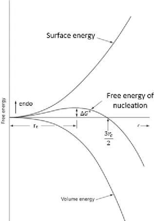
Figure 3.3. The free energy of a nucleation of a particle as a function of its radius. ... 41

Figure 3.4. Example for the first comparisons between simulated and experimental DSC curves of AA3105 at 5 K/min. ... 44

Figure 3.5. The evolution of (a) mean radius and (b) number density of the β” and β’ particles at 185 °C respectively. ... 45

Figure 3.6 The simulated and experimental DSC curves of an AA6016 aluminum alloy with a heating rate of with (a) 5K/min and (b) 10 K/min, an AA6005 aluminum alloy with a heating rate of with (c) 0.6 K/min and (d) 6 K/min and an AA3105 aluminum alloy with a heating rate of with (e) 0.6K/min and (f) 1.2 K/min respectively. ... 48

Figure 3.7. The simulated and experimental enthalpy change with and without considering GP zone and primary precipitates for (a-b) an AA6016 aluminum alloy with a heating rate of with 5K/min, (c-d) an AA6005 aluminum alloy with a heating rate of with 0.6 K/min and (e-f) an AA3105 aluminum alloy with a heating rate of with 0.6K/min respectively. ... 49

Figure 3.8. Simulated (a,b) particle number density, (c,d) mean radius and (e,f) phase fraction for a heating rate of (a,c,e) 5 K/min and (b,d,f) 10 K/min. ... 50

Figure 3.9. The simulated (a,b) particle number density, (c,d) mean radius and (e,f) phase fraction for a heating rate of (a,c,e) 6.0 K/min and (b,d,f) 0.6 K/min of AA6005 aluminum alloy. ... 51

(11)

viii

Figure 3.10. The simulated (a,b) particle number density, (c,d) mean radius and (e,f) phase fraction for a heating rate of (a,c,e) 1.2 K/min and (b,d,f) 0.6 K/min of AA3105 aluminum alloy. ... 52 Figure 3.11. The simulated isothermal heat treatment of AA3105 aluminum alloy at 265°C. 53 Figure 3.12. A Phase diagram of precipitation and dissolution of a β’ from aluminum matrix. ... 55 Figure 4.1. (a) The experimental DSC curves of the AA3105 alloy at 0.01 K/s in as-cast condition (Measurement performed by R. H. Kemsies) and (b-f) the dark-field and SAED pattern of the samples, which are quenched at 240, 300, 375, 405 and 500 °C, respectively. (Image acquired by S. Zischke) ... 61 Figure 4.2. (a) experimental DSC curves of the AA3105 alloy with 0.01 K/s in as-cast condition (Measurement performed by R. H. Kemsies) and (b-e) the dark-field and SAED pattern of the samples which are quenched at 310, 400, 460 and 550 °C, respectively. (Measurement performed by S. Zischke) ... 63 Figure 4.3. TEM dark-field micrograph of the AA3105 alloy after continuous heating to (a) 375 °C and (b) 405 °C. (Image acquired by S. Zischke) ... 64 Figure 5.1. Diffusion time vs. Temperature of Fe atoms for 100 nm diffusion distance. ... 68 Figure 5.2. The hardness results of the commercial AA3105 alloy in an as-cast condition with heat treatment path A, (a) cast in a sand mold, (b) cast in a copper mold; (c) optimized AA3105 in a copper mold. ... 69 Figure 5.3. (a,b) The conventional TEM image and (c,d) diffraction pattern of the optimized AA3105 in a copper mold which are quenched at 250 °C after (a,c) 10 hours and (b,d) 20 hours, respectively. Specific diffraction pattern were not recognized but the morphology of the particles suggests that they are β’’ and β’ precipitates. (TEM performed by S. Zischke) ... 70 Figure 5.4. The hardness results (a) of the commercial AA3105 alloy in an as-cast condition in a sand mold, (b) of the optimized AA3105 in a copper mold with path B and (c) The heat treatment path B. ... 71 Figure 5.5. The hardness results (a) of the commercial AA3105 alloy in an as-cast condition in a sand mold, (b) of the optimized AA3105 in a copper mold with path C and (c) The heat treatment path C. ... 72 Figure 6.1. Geometry of the tensile samples in units of mm. ... 75

(12)

ix

Figure 6.2. (a) HAADF image and (b) Line scan of X-ray spectrum of a dispersed particles. The main elements are: Al, Si, Mn, Mg and Fe. (TEM performed by S. Zischke) ... 76 Figure 6.3. (a) The conventional TEM micrograph and (b) the SAED pattern of the same area of the heat treated sample at 140 °C for 1000 hours. (Image acquired by S. Zischke) ... 77 Figure 6.4. Creep strain over time for the AA3105 aluminum at different temperatures. ... 78 Figure 6.5. (a) The strain rate raised to the power 1/n as a function of stress at 200 °C. b) the comparison between temperature dependence of normalized threshold stress and those predicted from various models proposed for dispersion hardened alloys [187]. ... 80 Figure 6.6. The minimum creep rates vs. reciprocal temperature at different stresses for AA3105 aluminum alloy. ... 81 Figure 6.7. The minimum creep rates vs. normalized stress at different temperatures a) without considering the threshold stress and b) with considering threshold stress for AA3105 aluminum alloy. ... 81 Figure 6.8. (a) The EBSD map, (b) histogram of the misorientation angle from 2-65° and (c-d) TEM dark-field micrograph of the extruded AA3105 aluminum alloy in the initial condition. (SEM performed by S.J. Schröders) ... 82 Figure 6.9. TEM dark-field micrographs of the crept AA3105 aluminum alloy (a) under 40 MPa after 14 hours and (b) 85 MPa after 2 hours at 175 °C. The arrows show areas with high dislocation density. (TEM performed by S. Zischke) ... 83 Figure 6.10. TEM dark-field micrograph of the crept AA3105 aluminum alloy under 40 MPa (a-b) after 1 h and (c-d) after 14 h at 175 °C. The arrows show dislocation pile-up and also dislocation dipoles. (Image acquired by S. Zischke) ... 84 Figure 6.11. (a-b) Kernel average misorientation angle maps and (c-d) histograms of the misorientation angle from 2-65° of the crept AA3105 aluminum alloy at 175 °C under 40 MPa after (a,c) 1 h and (b,d) 14 h. (SEM performed by S.J. Schröders) ... 85 Figure 6.12. TEM dark-field micrographs of the crept AA3105 aluminum alloy at 175 °C under 85 MPa after (a,b) 25 mins and (c,d) 2 h. The arrows show dislocations pile-up behind a precipitate and a subgrain formation. (Image acquired by S. Zischke) ... 86 Figure 6.13. (a-b) Kernel average misorientation angle maps and (c-d) histograms of the misorientation angle from 2-65° of the crept AA3105 aluminum alloy under 85 MPa load after (a,c) 25 mins and (b,d) 2 h. (SEM performed by S.J. Schröders) ... 87

(13)

x

Figure 6.14. The creep strain over time for the Al-Zr-Fe aluminum at different temperatures. ... 91 Figure 6.15. The minimum creep rates vs. reciprocal of the absolute temperature at different stresses for Al-Zr-Fe aluminum alloy. ... 92 Figure 6.16. The temperature dependence of minimum creep rates at different tensile stresses, to determine Q-values for Al-Zr-Fe aluminum alloy. ... 92 Figure 6.17. (a) SEM image, (b) EBSD map, (c) the EDS analysis and (d) histogram of the misorientation angle from 2-65° of the Al-Zr-Fe aluminum alloy in as-extruded condition. .. 94 Figure 6.18. TEM dark-field micrographs of the crept Al-Zr-Fe aluminum alloy at 125 °C (a,b) under 40 MPa and (c,d) 75 MPa in the steady-state region. Arrows show subgrain boundaries and dislocation dipoles. (Image acquired by S. Zischke) ... 95 Figure 6.19. (a-b) Kernel average misorientation angle maps and (c-d) histograms of the misorientation angle from 2-65° of the crept Al-Zr-Fe aluminum alloy at 125 °C (a,c) under 40 MPa and (b,d) 75 MPa in the steady-state region. (SEM performed by S.J. Schröders) .... 96 Figure 6.20. TEM dark-field micrographs of the crept Al-Zr-Fe aluminum alloy at 175 °C (a-b) under 40 MPa and (c-d) 75 MPa in the steady-state region. Arrows show subgrain boundaries, dislocations and low angle grain boundaries. (TEM performed by S. Zischke ) ... 97 Figure 6.21. Kernel average misorientation angle maps and histograms of the misorientation angle from 2-65° of the crept Al-Zr-Fe aluminum alloy at 175 °C (a,c) under 40 MPa and (b,d) 75 MPa in the steady-state region. (SEM performed by S.J. Schröders) ... 98 Figure 6.22. The temperature compensated strain rate vs. normalized stress for AA3105 and Al-Zr-Fe aluminum alloys. ... 100

(14)

xi

List of tables

Table 2.1. Creep parameters n, p and Q for different creep regimes [118]. ... 25 Table 3.1. List of the parameters used in the simulations ... 44 Table 4.1. The chemical composition of the AA3105 aluminum alloy with and without Mg addition ... 59 Table 5.1. The chemical composition of the commercial and optimized AA3105 aluminum alloy. ... 67 Table 6.1. The chemical composition of the extruded aluminum alloy. ... 74 Table 6.2. n, p and Q values for creep in pure aluminum ... 89

(15)

xii

List of symbols

𝜀̇ Strain rate / steady-state creep rate

𝜎 Stress

𝐷_𝑙 Lattice diffusion coefficient

𝐷_𝑏 Grain boundary diffusion coefficient

𝐷𝑝𝑑 Dislocation pipe diffusion coefficient

Ω Vacancy volume

𝐺𝑆 Grain diameter

𝑇 Temperature

𝑘 Boltzmann’s constant

𝐴𝐻𝐷 , 𝐴0 Constant

𝜎_𝑇ℎ Threshold Stress (MPa)

N Creep exponent

Q0 Self-diffusion activation energy

B Burgers vector

R Universal gas constant

G Shear modulus

P Pressure

𝜇 Chemical potential

V Volume

Vm _{Molar volume}

N Number of individual phases

N0 Nucleation sites

𝛾 Interfacial energy

𝜙 Heat flow

Cp Specific heat capacity

H Specific enthalpy

𝐺𝑠𝑦𝑠 Gibbs energy per unit volume of the system

∆𝑔_𝑝 Difference of Gibbs molar energy

σy Yield stress

(16)

1

1 Motivation

Copper alloys have an excellent electrical conductivity and, for this reason, have been used widely for many years in power grids. However, the price of the copper alloys has increased over time and a demand for new non-copper based conductive alloys has risen. The new alloys should satisfy the required mechanical and electrical properties. The new alloys must have high or comparable creep resistance, because the working temperature of the power grids remains normally at 140 °C but can increase for short periods to 200 °C. Additionally, new alloys should have high electrical conductivity and a reasonable price. Aluminum alloys are among the most promising candidates.

Aluminum has a high electrical conductivity (2.65×10-8 Ω.m), which satisfies this requirement for power grids. On the other hand, creep mechanisms in aluminum alloys are active at temperatures of more than approximately 0.5 of the homologous temperature, which is equal to 193.65 °C for pure aluminum, which is in the range of the working condition of the power grids. In order to use aluminum alloys in the power grids, it is necessary to develop alloys with an improved strength and creep resistance through different strengthening mechanisms. There are different strengthening mechanisms such as work hardening, solid solution hardening, precipitation hardening and dispersion hardening. Work hardening cannot in practice be considered, because the material recovers at operation temperatures. Solid solution hardening shows detrimental effects because high amount of substitutional or interstitial atoms decreases electrical conductivity. Therefore, solid solution hardening (dilute alloys), dispersion and precipitation hardening are the only possible useful mechanisms that can be applied. Nevertheless, the typical age hardening aluminum alloys are not useful in power grids, because the precipitates must be highly stable at the relatively high operation temperatures. To meet these requirements only a handful of elements can be considered. These elements are Cr, Cu, Fe, Mg, Mn, Ni, Si and Zr. Based on the mentioned elements, new aluminum alloys were produced and investigated in the frame of ALLEE project. The produced aluminum alloys were AA1070 (as a reference for the best electrical conductivity in aluminum alloys), AA6101A, AA8076A, AA3105, AA6101 + Zr, AA6101 + Ni and different alloys in AlNi, AlNiFe, AlZr and AlZrFe systems.

In order to achieve our goal and have a well-directed structure, the following questions are going to be examined in this dissertation in three chapters.

(17)

2 1.1 Scientific questions

1- How can precipitation be simulated and which classical nucleation and growth models can simulate the growth and dissolution kinetics of metastable phases? Can DSC curves be used to calibrate these models and is this kind of calibration preferable to microscopy imaging techniques? If so, is DSC sufficient? How far can this method substitute other experimentally expensive techniques?

In order to predict the correct sequence of metastable phases, a model is needed which should contain nucleation, growth and incubations models. The usual Zener growth law is not able to simulate the dissolution of the particles at lower temperatures compared to the phase diagram. In order to solve this problem, another growth law has to be implemented in the code. Furthermore, the model needs calibration. Calibration used to be based on TEM investigation which was time consuming. However, DSC curves could be useful tools to validate the precipitation sequence. DSC experiments show the precipitation sequence and the nucleation, growth and dissolution of the precipitates. Increasing the heating rate increases nucleation, growth and dissolution temperatures and shifts the DSC curves to higher temperatures.

A common method to calibrate this kind of models is TEM investigations, in which the phases, the size of the precipitates, are determined. But it is time consuming and costly. The DSC measurement can be a useful method to calibrate a model and reduce the TEM measurements.

2- Can a simulation model help to tune alloys, old or newly designed for preselected properties, in particular creep resistance and conductivity?

In order to obtain the maximum precipitation hardening, the precipitates should have a certain size (r0), which corresponds to the particle radius at which the Orowan and the cutting

stresses for dislocations to cut particles are equal.

Models for the prediction of the yield stress and the hardness were also implemented in the code to calculate the yield stress and consequently the hardness of the materials. Therefore, the maximum yields stress during a heat treatment can be calculated and the results are helpful to tune the strength of the simulated alloys. There are also functions to simulate the electrical conductivity of the alloys based on the chemical composition of the materials.

(18)

3

3- Which creep mechanisms are active at the application temperature and under different stresses? How can we optimize the creep resistance of aluminum alloys without compromising the electrical conductivity?

To address this question, the creep mechanisms which are active at the application temperature should be determined through creep tests at different temperatures and stresses. TEM investigations should prove if the defined creep mechanisms through the creep tests are valid. If dislocation glide is the dominant creep mechanism, solid solution hardening (dilute alloys), dispersion hardening and precipitation hardening could be helpful strengthening mechanisms to produce new aluminum alloys, which are creep resistant and have a comparable electrical conductivity with the copper alloys.

(19)

4

2 Literature review

2.1 Precipitation hardening in aluminum alloys 2.1.1 Precipitation hardening

One of the most important processes for strengthening materials is age hardening. Through age hardening the strength/density ratio increases, which is an important parameter in the aerospace industry. Age hardened aluminum alloys are also the base materials used in automotive applications. Precipitation hardening is the principle of age hardening, in which second phase particles precipitate from a supersaturated solid solution. Precipitates and matrix interface can be coherent, partially coherent or incoherent. The type of interface can determine decisively how a dislocation interacts with a precipitate (e.g. [1]–[5]).

If a quenched super saturated solid solution is tempered at low temperatures, metastable phases can appear. These particles usually have coherent or partially coherent phase boundaries. In such cases, dislocations commonly cut the particles (see Figure 2.1.a). This process will produce new interfaces, which increases the free energy of the crystal. This energy must be compensated by the applied stress causing the dislocation motion[1]. The strengthening contribution of the particles when cut depends on the particle radius and their volume fraction (Eq. 1) (e.g. [1]):

Eq. 1 ∆𝜏_𝑐 = 𝛾̃3 2⁄ 𝑏 √𝑓 √𝑟 √6𝐸𝑣 ̅̅̅̅̅̅̅

where 𝑓 is volume fraction, 𝛾̃ is an effective interface energy, 𝑟 is the particle radius and 𝐸𝑣 is

the energy of an edge dislocation. If the heat treatment is conducted for a long time, the metastable particles grow and transform into stable phases that form incoherent boundaries with the matrix. In this case, the dislocations can only bypass the particles (see Figure 2.1.b) [1]. The stress which is necessary for dislocations to bypass particles, can be calculated according to Orowan mechanism (Eq. 2) as [1]:

Eq. 2 𝜏_𝑂𝑅 = 𝐺𝑏

𝑟 √𝑓

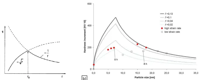
Figure 2.2.a shows the theoretical dependence of strengthening on particle size. There is always an optimum radius (Eq. 3) which delivers the maximum strength [1].

Eq. 3 𝑟_𝑐 = 𝐺𝑏2

𝛾̅ √3

(20)

5

If the precipitates are smaller than rc, dislocations pass them by cutting and if their radius is

bigger than rc, they will be by passed by the Orowan mechanism[1]. Figure 2.2.b shows the

effect of particles’ volume fraction on the Hardness [6].

Figure 2.1. A dislocation-particle interaction (a) by the cutting mechanism (b) by Orowan’s mechanism [1], [2].

Figure 2.2. The dependence of strengthening on particle size. (a) Schematic from theories; (b) effect of particles’ volume fraction on the Hardness [6].

2.1.1.1 2xxx, 6xxx and 7xxx series aluminum alloys

Typical examples of age hardenable aluminum alloys are the 2xxx series aluminum alloys containing Cu and Mg with copper as the major alloying element. Additionally, 6xxx series aluminum alloys containing Mg and Si have been considered as the most promising age-hardenable materials for automotive applications as well as the 7xxx series aluminum alloys containing Zn, Mg and Cu with zinc as the major alloying elements [1], [7]–[10].

The 2xxx series aluminum alloys become hardenable mainly by the addition of Cu [11]–[14]. The maximum solubility of Cu in Al is 5.56% at 548 °C and it decreases to less than 1% at room temperature. In order to observe the age hardening effect, the chemical composition of the

a) b)

(21)

6

alloy must be in a composition range that at high temperatures allows all the elements to be in a solid solution whereas at lower temperatures the solid solution decomposes into two phases. Figure 2.3.a shows the Al-Cu phase diagram on the Al-rich side. If a sample with a composition close to the a-b-c line in Figure 2.3 is quenched after homogenization at 548 °C, it will result in a super saturated solid solution. Afterward, if the sample is heat treated at temperatures higher than room temperature but substantially lower than the solvus temperature, the hardness of the sample will increase due to the nucleation and growth of particles of a secondary phase (see Figure 2.3.b). The first hardening stage can be attributed to the GP zones formation. By increasing time or temperature, a second peak is observed. This is caused by the formation of 𝜃′ phase. If the heat treatment continues further, the precipitates grow further and the hardness decreases due to the Ostwald ripening [15]. The sequence of formation of precipitates in 2xxx series aluminum alloys was described by GPI+GPII zones → θ′ → θ (Al2Cu) or GPII zones → S’′ → S’ → S1 and S2 (Al2CuMg)[1], [16]. The

formation of the S or θ phase depends on the chemical composition of the alloy. Artificial ageing can be done at the range of 130-170 °C for 2xxx series aluminum alloys [17]–[20].

Figure 2.3. (a) The Cu phase diagram o the rich side, (b) age hardening curves of AI-4%Cu-l%Mg [1], [21].

The 6xxx series aluminum alloys have been also the subject of several studies in recent years. In particular, Al-Si-Mg alloys have displayed excellent mechanical properties owing to substantial age-hardening upon heat treatment [3], [22]–[28]. These alloys are used widely for automotive and aircraft applications. In commercial 6xxx series aluminum alloys, the amount of magnesium and silicon content are set in such a way that allows forming a

(22)

7

binary Al–Mg2Si alloy (Mg:Si 1.73:1). It is also possible to permit an excess of silicon, which is

needed to form Mg2Si. To tailor the mechanical properties in these alloys, it is essential to

know the exact precipitation sequence and their corresponding kinetics of precipitation and growth. In this regard, there have been experimental investigations that have showed that the precipitation hardening response is related to the Mg-Si phases [9], [29]–[31]. The sequence of precipitation formation from the solid solution condition in Al-Mg-Si alloys can be described as cluster → GP zones → β′′ → β′ → β (Mg2Si), whereas the precipitation sequence of

Al-Mg-Si alloys with a high silicon content is believed to be GP zones → small precipitates with an unknown structure → β′′ → β′ → Si → β (Mg2Si) [32]–[38].

The metastable precipitates are in nano-scale, therefore TEM is used to characterize them. Figure 2.4 shows the bright field image of an AA6022 aluminum alloy, which is heat-treated to 260 and 300 °C at 10 °C/min after solutionizing and quenching [39]. TEM images have shown that at 260 °C the precipitates are needle-like, between 20-40 nm long and with a diameter between 2-5 nm. The overlap of diffraction patterns of the precipitates on the matrix diffraction pattern can be observed along [010]Al zone axis due to the needle-like morphology of the precipitates. The cross section of the precipitates of the quenched sample at 300 °C is rectangular. This shape has been attributed to the β′ lath-like precipitates [28], [30], [39], [40].

In the as-cast condition, there are two types β precipitates. They are shown in Figure 2.5. One type is shown to precipitate on the boundaries of the primary solidified α-Al(Mn,Fe)Si particles. The mentioned precipitates are spherical and generally bigger than 2µm. The second ones are observed to appear in the matrix. These particles precipitate from the super saturated solid solution. These latter precipitates are plate-like or needle-like and usually smaller than 0.5 µm. It is also stressed that higher content of the Fe leads to a lower volume fraction of the Mg-Si phases. This is attributed to the absorption of the Si by α-Al(Mn,Fe)Si phase and consequently lower Si content available in the matrix for the formation of the particles Mg-Si particles [41].

(23)

8

Figure 2.4. Bright-field TEM micrographs ([001]Al zone axis) of a AA6022 aluminum alloy heated to (a) 260 °C and (b) 300 °C at 10 °C/min immediately after solutionizing and quenching [39].

Figure 2.5. Optical micrographs of an Al-Mg-Si alloy [41].

In order to determine the precipitated phase in the matrix, a selected area electron diffraction (SAED) pattern of the precipitates must be compared with known structures. Figure 2.6 shows the predicted diffracted pattern of a [001] Al zone axis which contains needle-like precipitates along the [010] and [100] zone axis of matrix. This pattern should be compared with the experimental SAED patterns from the precipitates [30]. The structure of metastable and stable Mg-Si phases are discussed in [28], [42].

a) b)

(24)

9

Figure 2.6. Predicted diffracted patterns of (a) a [001]Al zone axis which contains needle-like precipitates β’’ along [010] and [100] zone axis of matrix [30] (b) β’ and Q’ with a same orientation relation[28].

The 7xxx series aluminum alloys deliver the highest precipitation hardening contribution among all aluminum alloys. 7xxx series aluminum alloys contain Zn and Mg. The sequence of precipitation formation from the solid solution in Al-Zn-Mg alloys is described as: solid solution → GP-zones → η’ → η -MgZn2 [43]–[47]. Studies have shown that the highest

contribution of the particles on the strengthening of the 7xxx series aluminum alloys is observed after a single ageing at temperatures in the range 120–135 °C. At higher temperatures of 160-170 °C, the strength of the material decreases drastically due to the formation of η or η’ phases [9].

The 3xxx series aluminum alloys have been used widely in packaging. The 3xxx series aluminum alloys are denoted as non-heat treatable alloys. The diffusion of Fe and Mn, which are the main alloying elements in the 3xxx series aluminum alloys, are rather low in the aluminum matrix. Therefore, the usual strengthening mechanism in these alloys is work hardening [48]–[50]. However recent reports have shown that a precipitation process occurs in an as-cast AA3004 alloy and improves the mechanical properties and electrical conductivity [51]–[57]. The partially coherent α-Al(Mn,Fe)Si dispersoids precipitated during heat treatment and simultaneously primary Al6(Mn,Fe) particles dissolved [58]–[60]. Figure 2.7

shows a 3D representation of the diffraction pattern. It indicates the dissolution and precipitation of different phases during heating at 50°C/h up to 550°C for a 3003 aluminum alloy [59].

(25)

10

Figure 2.7. 3D representation of the diffraction pattern of a 3003 aluminum alloy during continuous heating at 50°C/h up to 550°C [59].

2.2 Differential scanning calorimetry

Owing to the difficulty of directly observing the precipitation sequence, differential scanning calorimetry has been used to determine the temperatures associated with precipitation and thus capture the precipitation behavior indirectly [28], [35], [39], [61]–[67]. The method was developed in 1962 by E. Watson [68]. In this method, a sample and a reference material are heated simultaneously. During the heating of the sample, different physical transformations can occur. These transformations release or absorb energy and thus influence the temperature. Simultaneously, the differences between the sample’s temperature and the temperature of the reference material are recorded. The recorded data can be converted to energy changes, which occur in the samples during heating or cooling. During a DSC measurement, the temperature is increased with a constant rate with respect to the time. As long as no reaction happens in the sample, the temperature difference of the sample and the reference material is zero. If an endothermic transformation occurs, the sample absorbs energy and causes a delay in the temperature rise. When the transformation is completed,

(26)

11

the system goes back to a dynamic equilibrium condition, meaning that the sample temperature change approaches that of the reference material. If the transformation is exothermic, the sample temperature rises and for a while, the temperature of the sample is higher than the reference material [68]. The result of the DSC measurement is a curve of heat flow with respect to temperature. An advantage of DSC measurements is that the recorded curves shows clearly the precipitation and dissolution of precipitates [63], [69]. As an example, Figure 2.8 shows the DSC curve of an Al-Mg-Si alloy at different heating rates. The first exothermic peak A is attributed to the formation of solute atom clusters. Peak B shows the dissolution of them. Peak C is due to the β’’ precipitates which are needle-like. The next peak D is interpreted as the growth process of β’’ needles into β’ rods. The reaction E is probably from the β-Mg2Si precipitation. It is also known that the excess Si accelerates formation of

cluster or β’’. Figure 2.8 shows that increasing the heating rate shifts the peaks to higher temperatures [34], [36].

Figure 2.8. DSC curves of an Al-Mg-Si alloy at different heating rates [34].

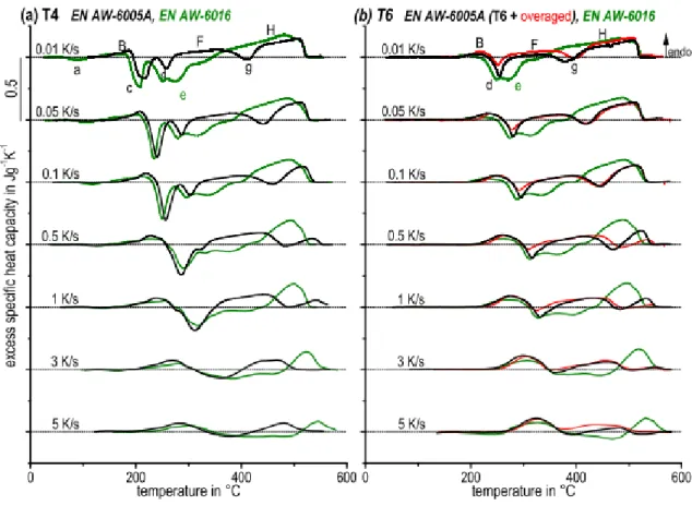
Osten et al. [70] investigated the effect of different heating rates on the precipitation sequence and dissolution of particles in different 6xxx series aluminum alloys. They reported that the initial microstructure affected strongly the dissolution and precipitation behavior of the materials. Figure 2.9 shows the DSC curves of AA6005A and AA6016 with different heating rates for the same initial conditions. The peaks shifted to higher temperatures by increasing the heating rate. It has been claimed that the area under the peaks decreases by increasing the heating rates [70]. This is attributed to the suppression of the diffusion process. When the heating rate is higher, the precipitation sequence cannot be completed. Additionally, the

(27)

12

precipitation and dissolution processes are diffusion controlled processes and their dependency on heating rate is observable by following the evolution of peak H at different heating rates in Figure 2.9. When the heating rate is higher, there is not enough time for diffusion and the peaks are smaller and are shifted to higher temperatures. The different height of the peaks c and d is related to the overlap of exothermic and endothermic reactions, in which a faster dissolution kinetic and slower precipitation reaction are superimposed[67], [70]. The kinetic and precipitation sequence of the T6 (artificially aged conditions) and the T4 (naturally aged) conditions are similar. Specifically, there are no peaks a and c. This is because of precipitation of GP zones and β′′, which formed previously during the T6 process. These particles are dissolved at T4. The further sequence correlates with the development of the T4 natural aged condition. In order to show the different initial conditions, different aluminum alloys were used. For a higher content of Mg and Si, formation of clusters (peak a) is observed in the EN-AW6016 specimens in T4 condition. This peak followed the endothermic peak B, which is attributed to the dissolution of the clusters. The peaks c and d were reported frequently as formation of β”and β’ precipitates. Consequently, peaks F and H are endothermic reactions of the dissolution of these precipitates and g is the exothermic peak of β formation. According to the EN-AW6016 samples, by overlapping of the dissolution and precipitations, the peak formation of β was not observed.

This analysis shows that DSC is a powerful method to observe the precipitation kinetic in materials, however it is necessary to use alternative methods to determine the phases which are precipitated at certain temperatures.

2.3 Modelling of precipitation

Formation of new particles from a super saturated solid solution is termed precipitation and can be considered as a reaction in a closed region in space and described in a thermodynamic system. The free energy of the thermodynamic system, which is described by Gibbs free energy G, can be considered as the driving force of the phase transformation[71]:

Eq. 4 𝐺 = 𝑈 + 𝑃𝑉 − 𝑇𝑆

where U internal energy, P and V are pressure and volume. T is temperature and S is entropy. The partial derivatives of the Gibbs free energy with respect to the states parameter are[71]:

(28)

13

Figure 2.9. DSC curves of AA6005A and AA6016 with different heating rates for the initial conditions (a) T4. (b) T6 [70]. Eq. 5 (𝜕𝐺 𝜕𝑇)_𝑃,𝑁_𝑖 = −𝑆 Eq. 6 (𝜕𝐺 𝜕𝑃)_𝑇,𝑁 𝑖 = 𝑉 Eq. 7 (𝜕𝐺 𝜕𝑁𝑖)_{𝑇,𝑃,𝑁} 𝑗≠𝑖 = 𝜇_𝑖

Here 𝜇𝑖 is chemical potential of component 𝑖 and 𝑁𝑖 is the number of moles of component 𝑖.

The precipitation process is considered in an isothermal and isobaric system. Therefore, the chemical potential in the Eq. 7 is more important for the precipitation process. The Gibbs energy of a system is described by the summation of the chemical potential of all the components[71].

Eq. 8 𝐺 = ∑ 𝜇𝑖 𝑖𝑁𝑖

(29)

14

Figure 2.10 shows a typical sketch of Gibbs energy vs composition. The driving force for the precipitation of the β phase (𝑑_{𝑐ℎ𝑒𝑚}𝛽 ) from a super saturated solid solution is described by Eq. 9 [71]:

Eq. 9 𝑑_{𝑐ℎ𝑒𝑚}𝛽 = − ∑ 𝑋𝑖 _𝑖𝛽(𝜇_𝑖𝛽− 𝜇_𝑖𝛼)

where 𝑋_𝑖𝛽 is molfe fraction of phase 𝛽.

Figure 2.10. A typical Gibbs energy vs composition with an evaluation procedure for driving force calculation [71].

Beside the chemical driving force, the capillary force and the elastic misfit stress (∆𝐺_𝑣𝑜𝑙𝑒𝑙 ) reduce the driving force for precipitation. The capillary force stems from the pressure exerted by the curvature of the interface on its surface. The second back driving force is the volumetric lattice mismatch between matrix and precipitate that causes an elastic distortion and thus, an increase of the free energy in the system[71].

2.3.1 Nucleation of precipitates

In 1935 Becker and Döring [72], [73] introduced a kinetic equation for the nucleation of droplets from a super saturated vapor. This equation has been proven to be valid as long as the amount of the phases are not comparable to each other. It is necessary to know the total formation energy of a spherical nucleus to calculate the energy barrier at critical radius Δ𝐺∗

Eq. 10 𝛥𝐺∗_{(𝑟) = ∆𝑔} 𝑇∙ 4𝜋 3 𝑟 3 _{+ 𝛾 ∙ 4𝜋𝑟}2

(30)

15

where γ and ∆𝑔𝑇 are the interfacial energy and chemical driving force per volume. 𝑟 is the

radius of the particle. The total formation energy has a maximum value, which can be calculated according to the Eq. 12. The critical radius is the radius of nucleus at the maximum value which can be calculated using Eq. 10.

Eq. 11 𝑟∗ = 2.𝛾 𝑑 𝑐ℎ𝑒𝑚 𝛽 𝑣𝛼 −∆𝐺𝑣𝑜𝑙 𝑒𝑙 Eq. 12 ∆𝐺∗ = 16𝜋.𝛾3 3.(−𝑑𝑐ℎ𝑒𝑚 𝛽 𝑣𝛼 +∆𝐺𝑣𝑜𝑙 𝑒𝑙 ₎ 2

Here 𝑣𝛼and ∆𝐺_𝑣𝑜𝑙𝑒𝑙 are the molar volume of a phase and the elastic energy per volume, respectively. The probability of a thermal fluctuation to be sufficient for nucleation is calculated by an Arrhenius term, hence the nucleation rate (J) can be written as:

Eq. 13

𝐽 = 𝑁̇ exp (−∆𝐺∗

𝐾𝐵𝑇)

where 𝑁̇ describes the density and frequency of nucleation attempts, which will be discussed in detail for the ClaNG model [71].

2.3.2 Growth and coarsening of precipitates 2.3.2.1 Zener growth model

The first theory of coarsening was proposed by Lifshitz and Slyozov [74]. Almost simultaneously, Wagner described the coarsening with another model [15]. The Lifshitz model was based on Zener’s growth law. Zener’s growth law is valid for spherical precipitates in a binary alloy and is described by [75], [76]:

Eq. 14 𝑑𝑟 𝑑𝑡 = 𝐷𝑖 𝑟 𝐶𝑖𝛼−𝐶𝑖 𝛼 𝛽⁄ (𝑟) 𝐶_𝑖𝛽−𝐶_𝑖𝛼 𝛽⁄ (𝑟)

Here 𝐷𝑖 is diffusion coefficient of element 𝑖 in matrix. 𝐶𝑖 𝛽

(𝑟) and 𝐶𝑖𝛼(𝑟) are the concentration

of element 𝑖 in the particle and in the matrix. 𝐶_𝑖𝛼 𝛽⁄ (𝑟) is the concentration of element 𝑖 at the particle interface in the matrix and can be calculated by the Gibbs-Thomson equation. The Gibbs-Thomson equation describes the effect of the curvature at the interface. According to Zener’s law, the equilibrium concentration is only valid for a planar interface. The Gibbs-Thomson equation can be described by [75]–[78]:

(31)

16

Eq. 15 𝐶_𝑖𝛼 𝛽⁄ (𝑟) = 𝐶_𝑖𝛼(𝑟). 𝑒𝑥𝑝 (2𝛾.𝑉_{𝑅𝑇.𝑟}𝑚)

2.3.2.2 SFFK growth model

In 2004, Svoboda, Fischer, Fratzl and Kozeschnik developed a new growth model based on the mean chemical composition of the matrix. This model is valid for all stages of the evolution of the particles in a multi component system. It applies the extremum principle on the Gibbs function and has proven to be in good agreement with other established simulation techniques [79], [80]. Eq. 16 gives the growth rate of the precipitates in the SFFK model.

Eq. 16 𝑟̇ = ∆𝑔𝑇−( 2𝛾 𝑟) 𝑅𝑇𝑟 [∑ (𝐶_𝑖𝛽−𝐶𝑖𝛼) 2 𝐶_𝑖𝛼𝐷𝑖 𝑛 𝑖=1 ] −1 2.3.3 Data representation

The first implemented nucleation and growth model was reported by Langer and Schwartz. They considered the processes of nucleation, growth and coarsening to proceed simultaneously. Their model describes droplet formation and growth in near critical fluids [81]. The model delivers a time evolution of droplet density and mean radius. Later, the Langer and Schwartz model was improved by Kampmann and Wagner [82] using a model for a supersaturated solid solution. In the mentioned models, a single radius was used instead of a precipitation size distribution. Later on, Wagner and Kampmann introduced a size distribution to their model. The model can predict the evolution of the precipitation size distribution [83]. The evolution of the precipitation size distribution can be implemented with different approaches. For instance, the mean radius approach, Lagrange-like approach and Euler-like approach are three methods for the implementation of the radius of the precipitates in the model. In simple cases, they deliver the same results but in more complex situations multi-class approaches are necessary [84]. In the following two multi-multi-class approaches will be explained.

2.3.3.1 Euler-like approach

In this method, the precipitation size distribution is discretized in several size classes, and there is a flux of the particles occurring at the boundaries of the fixed classes as particles change their size. This is the method which Kampmann and Wagner used. Later on, Myhr et al. proposed to keep the volume constant in the growth stage [85]. In this method, the time increments must be calculated in a way that the highest change in a precipitation radius is

(32)

17

equal to half of the class width. A new population of a class is calculated from the number density and growth rate of the neighbor classes. The shifted amount of precipitates at the boundaries is added to the neighboring classes. Figure 2.11 shows the growth of the particles in the Euler-like approach. The flux between neighbor classes is calculated at each time step [84].

Figure 2.11. The growth of the particles in the Euler-like approach[84].

2.3.3.2 Lagrange-like approach

Maugis et al. proposed the Lagrange-like approach [86]. In this approach, the population of the classes is unaffected by growth; only nucleation and dissolution affect the populations. Growth is considered by altering the size corresponding to each class. As usual, too short time steps lead to slow simulations, and too large time steps lead to numerical instabilities. Figure 2.12 shows the nucleation and growth steps within a Lagrange-like approach [84].

(33)

18 2.3.4 DSC modeling

DSC measurements are an excellent tool to validate simulation models. Understanding the precipitation kinetics during the isothermal and non-isothermal heat treatment is essential to predict microstructure evolution and tailor the alloy to specific applications. For this purpose, in recent years, the simulation of isothermal heat treatments has been investigated widely [75], [85], [87], [88]. However, simulations of non-isothermal heat treatments, which are more relevant for technical applications, have been less frequent, in particular, in conjunction with a comprehensive validation. This last point is very relevant because in most cases the validation of the models have relied on observations with poor statistics such as particle size or volume fraction, which are performed by TEM microscopy, owing to the very small size of the particles[88]. Evidently, dissolution and precipitation of phases are difficult to characterize accurately by this method. An alternative to this method is the use of DSC measurements that can capture such events depending on the type of the reaction. In fact, DSC curves have been frequently utilized to characterize phase transformations, and in the specific case of Al alloys, these curves have been even recently simulated. For instance, Khan et al. introduced a first model for the simulation of DSC curves [89], [90] that was used by Falahati et al. [91]–[93] to simulate DSC curves in two aluminum alloys, 6xxx and 2xxx. Khan et al. defined the heat flow 𝜙 as: Eq. 17 𝜙 = (𝑐𝑝 𝑠𝑦𝑠 − 𝑐𝑝𝐴𝑙) × ∆𝑇 ∆𝑡= 𝑑(ℎ𝑠𝑦𝑠−ℎ𝐴𝑙) 𝑑𝑇 × ∆𝑇 ∆𝑡

where 𝑐_𝑝𝑠𝑦𝑠 and 𝑐𝑝𝐴𝑙 are the alloy and pure reference aluminum specific heat capacities,

respectively; ℎ𝑠𝑦𝑠 and ℎ𝐴𝑙 are the alloy and pure Al specific enthalpies, respectively and ∆T/∆t is the heating rate. It is noted that in this model the effect of interfacial energy on the heat flow had not been considered.

Hersent et al. calculated the released and/or absorbed energy by using the classical Gibbs model [94]: Eq. 18 𝐺𝑠𝑦𝑠𝑤 = 1 𝜌( 𝑔_𝑠𝑠𝑚 𝑉𝑠𝑠𝑚+ ∆𝑔_𝑝𝑚 𝑉𝑝𝑚. 𝑓𝑣+ 𝛾. 𝐴 𝑉𝑠𝑦𝑠)

where 𝐺𝑠𝑦𝑠𝑤 is the total Gibbs energy per unit volume of the system, 𝑔𝑠𝑠𝑚 is the Gibbs molar

enthalpy, ∆𝑔𝑝𝑚 is the difference of the Gibbs molar energy between the precipitates and the

(34)

19

precipitates, respectively. 𝑓𝑣 is the volume fraction of the precipitates and 𝐴 is the total

interface area developed by the precipitates. These models or slight variations of them have been used to predict DSC curves. For instance, Starink et al. [89], [95] simulated the DSC curves of a 2024-T351 Al–Cu–Mg alloy using basically Khan’s model (Eq. 1). They studied also the effect of the heating rate, which shifts the peaks, in a 2024-T351 alloy. In their approach, they implemented a time delay which depends on the interfacial energy, which in turn varies with the temperature [89]. These models have simulated the DSC curves with good accuracy. However, it must be stressed that some improvements can still be done by considering the effect on the energy of nucleation at preexisting lattice defects and explicit incubation time models. In the present study, a new model to describe endothermic und exothermic reactions during heat treatment of Al-Mg-Si alloys was developed and DSC curves used for calibration.

2.4 Creep mechanisms in aluminum alloys

High creep resistance is important for the conductor metals in power grids, because of the high working temperatures and stresses, which leads to activation of the creep mechanisms. Creep is a deformation mechanism which occurs in metals at high temperatures under a constant load or stress[1], [96]. Creep is a thermally activated process. According to established understanding, it needs a high vacancy concentration and thermal movement of atoms. Figure 2.13.a shows a typical creep curve, which shows the strain with respect to time and Figure 2.13.b shows the strain rate as a function of time. Increasing the stress at a constant temperature or increasing the temperature at a constant stress decreases the steady-state creep region [1].

The creep deformation is divided into three areas:

1. Primary creep: The strain increases with decreasing strain rate

2. Secondary creep: The strain increases linearly with a constant strain rate

3. Tertiary creep: The strain increases exponentially with increasing strain rate until fracture

The secondary stage of creep (steady-state creep) is the most important stage. It depends on temperature and the applied stress[96]. Steady-state creep refers to the region in the creep curves in which essentially, the substructure is quasi-static as dislocation multiplication and dynamic recovery are in balance. Whereas, the substructure formation depends on the

(35)

20

formation of a dislocation network. The secondary creep refers to the same region in the curve and is a region between tertiary and primary creep [97]. If a second and tertiary creep stage is not clearly observed, the minimum creep rate is used instead. The steady-state creep rate 𝜖̇_𝑠 can be described as a function of stress σ (known as “power-Law”) and temperature T:

Figure 2.13. (a) A typical creep curve: strain as a function of time. (b) schematic curve of strain rate as a function of time [1].

Eq. 19 𝜖_𝑆̇ = 𝐴 𝜎𝑛exp (− 𝑄

𝑘𝑇)

where A is material and Temperature dependent [1]. The n-value is the creep stress exponent, Q is the activation energy and K is the Boltzmann constant.

There are different mechanisms which may contribute to creep. A common classification is dividing the creep mechanisms into: Dislocation creep, Grain boundary sliding and Diffusion flow caused by vacancies[98].

2.4.1 Dislocation creep

Dislocation motion is separated to two different types: slip and climb. Slip means dislocation motion in their slip planes. Whereas in climb, the motion is normal to the slip plane. If the stress is above the yield stress (on the order of a tenth of the theoretical shear strength (G/10), dislocation glide is the active deformation mechanism. If the stress is lower, as is usually the case in creep, continued slip of dislocations is only possible in combination with climb of the dislocations. In any case, whether the slip is accompanied with climb or not, dislocation

(36)

21

multiplication takes place with increasing strain. This leads to an increased critical stress, i.e. work hardening. In a creep experiment, the external stress is kept constant. This means that the creep rate decreases with increasing strain. However, there are also recovery processes, i.e. a reduction of dislocation density. When the dislocation multiplication and the recovery processes reach a balance, a quasi-steady state condition is reached. This is one possible explanation of the secondary creep stage.

Recovery is governed by the slip and climb of the dislocations, which also depends on the vacancies diffusion. It is common to consider the same activation energies for self-diffusion and for creep [98].

2.4.2 Grain boundary sliding

Grain boundary sliding (GBS) is known as a process in which the grains slide along their common boundaries (see Figure 2.14) [99]–[101]. Surface marker lines were used by Moore et al [102], [103] to observe the developed step at the intersection of the line with the grain boundaries. GBS was observed in different materials [104]–[106]. Grain boundary sliding is divided into Rachinger sliding [107] and Lifshitz [74] sliding. In Rachinger sliding, the grains keep their original shape, but they are displaced with respect to each other. This occurs under creep condition in polycrystalline samples when the number of grains increases along the tensile direction within the gauge length. The second one occurs in Nabarro-Herring and Coble diffusion creep and develops an offset between the markers as a direct consequence of the stress-directed diffusion of vacancies [108]. GBS may be responsible for 10—65% of the total creep strain. The contribution of the GBS to the creep strain increases with increasing the temperature and decreasing grain diameter[101]. The latter means that in order to minimize grain boundary sliding, the grains should be large. Unfortunately, this also means that any strengthening effect related to grain boundaries is not a good option to minimize creep. For instance, the Hall Petch stress increases the strength of the material at low grain diameters [109], [110], but at the same time low grain diameters promote higher creep rates due to grain boundary sliding. Additionally, grain boundaries are sources of vacancy formation, such that a higher amount of grain boundaries leads to higher vacancies presence, which will increase the dislocation climb[98]. Eq. 20 [111]–[113] and Eq. 21 [114] are models to calculate the steady-state creep rate in GBS.

Eq. 20 𝜀̇_(𝑑_𝑔_{<𝑠𝑢𝑏𝑔𝑟𝑎𝑖𝑛𝑠 𝑠𝑖𝑧𝑒)} = 𝐴′ (𝑏 𝑑⁄ _𝑔)2(𝜎 𝐺⁄ )2_(𝐷

(37)

22

Eq. 21 𝜀̇_(𝑑_𝑔_{>𝑠𝑢𝑏𝑔𝑟𝑎𝑖𝑛𝑠 𝑠𝑖𝑧𝑒)} = 𝐴′ (𝑏 𝑑⁄ _𝑔)1(𝜎 𝐺⁄ )3_(𝐷

𝑔𝑏Gb 𝑘𝑇)⁄

Figure 2.14. The occurrence of GBS revealed by the boundary offsets in a transverse marker line for an Mg-0.78%Al alloy tested under creep condition at 200 °C. The tensile axis is horizontal [101].

2.4.3 Diffusion flow caused by vacancies:

The diffusion creep mechanisms can be divided in three regimes, which are characterized by their stress exponents (see Figure 2.15). One for low stress exponent (n = 1-2), one for intermediate stress exponent (n = 4-5/3-6) and one for high stress exponent.

Figure 2.15. Creep regimes in dependence on stress. [96]

(38)

23 2.4.3.1 Nabarro-Herring creep

Nabarro reported that in polycrystalline materials, self-diffusion within the grains causes yielding. Nabarro claimed that the effective viscosity is proportional to the square of the grain diameter (𝑑𝑔). Figure 2.16 shows the self-diffusion path of the elements in this creep

mechanism. This phenomenon leads to creep at very high temperatures and very low stresses. Afterward Herring has explained that the presence of a pressure gradient leads to a diffusion flux of atoms in a direction which will relieve the inequality of pressure. This pressure gradient is energetically advantageous to move the lattice defects. In absence of a pressure gradient, diffusion flux of atoms is proportional to the gradient of the concentration of these lattice defects. Herring has proposed a model to calculate the steady-state creep rate Eq. 22 [115].

Eq. 22 𝜀̇ = 10 𝜎 𝐷_𝑙Ω (𝑑⁄ _𝑔)2𝑘𝑇

where Ω is the atomic volume and 𝐷𝑙is lattice diffusion coefficient.

Figure 2.16. The self-diffusion within grains which causes creep in polycrystalline materials [115].

2.4.3.2 Coble creep

In 1963 Coble has developed a model for grain boundary diffusion controlled creep in polycrystalline materials. Coble found that the diffusion coefficients calculated via the Nabarro-Herring model from experimental creep rates were much larger than the self-diffusion coefficients. He explained the discrepancy by the self-diffusion through the grain boundaries [116]. He found that the stress exponent for both the lattice and grain boundary diffusion is the same. Thus, the only method to distinguish between the models is the grain

(39)

24

diameter dependency. Coble proposed that the exponent p in 𝜎 (𝑑𝑔) 𝑝

⁄ is equal to 2 in the

lattice diffusion model, and equal to 3 for boundary diffusion (see Eq. 23).

Eq. 23 𝜀̇ = 148 𝜎 (𝐷_𝑔𝑏W) Ω (𝑑⁄ _𝑔)3𝑘𝑇

Here W is the effective boundary width and Dgb is the boundary diffusion coefficient.

2.4.3.3 Harper-Dorn creep

The Harper-Dorn creep mechanism is active at extremely high temperatures and at very low stresses, which explains the dislocation-climb theory. The Harper-Dorn mechanism is dominant in stress range up to 2.0 MPa [117]. Figure 2.17 shows the Harper-Dorn regime and Nabarro-Herring for different grain diameters for a pure Al [118]. The activation energy at high temperatures is equal to the activation energy for the self-diffusion mechanism, which is also the same as for the Nabarro-Herring creep mechanism, but the subgrain boundary formation shows that dislocation climb does occur. At high temperatures, the dislocations, which are piled up at the barrier, can escape the traps by climb. The observed steady-state creep is about 1400 times more than the Nabarro-Herring creep mechanism[117]. Yavari et al. [118] proposed the steady-state creep rate:

Eq. 24 𝜀̇ = 𝐴_𝐻𝐷 (𝜎 𝐺⁄ )1_(𝐷

𝑙Gb 𝑘𝑇)⁄

Figure 2.17. The temperature compensated shear strain rate vs. normalized shear stress (τ/G) for pure Al [118].

(40)

25 2.4.4 Low-temperature creep

In 2013, Matsunaga et al. reported that at low temperatures (Less than 0.4 melting temperature) a new creep mechanism can be active. This new creep mechanism was added to the deformation mechanism maps. Figure 2.18 shows the new deformation mechanism map[119]. The grain diameter exponent (p value) is equal to zero, which means that the new creep mechanism is independent of the grain diameter. The creep exponent is 4 and increases to 6 when the temperature increases and the activation energy is 30 kJ/mole. 30 kJ/mole is less than the self-diffusion activation energy and implies that the self-diffusion processes are not dominant [119]. The rate controlling process is dislocation annihilation by cross slip at cell walls (see Figure 2.19). Table 2.1 shows the exponents n and p and the activation energy for different regimes [119].

Figure 2.18. The re-drawn maps for 5N Al with d = 140 μm [119].

Figure 2.19. TEM images of cell walls taken after 8.6 × 105_{s creep under 30MPa at 300K}

for 5N Al [119].

(41)

26 2.4.5 Methods to improve creep resistance

Dislocation motion and diffusion are two main creep mechanisms that control the creep rate. Retarding the dislocation motion and diffusion are important to improve the creep resistance of alloys.

In order to reduce the dislocation motion under a certain stress, the metals with higher melting temperature are preferred. Additionally, introducing obstacles which increase the needed stress to move the dislocations through a lattice by the Orowan mechanism, is useful. Additionally, metals with bigger grain diameters contain less grain boundaries, which are considered as fast diffusion paths. A larger grain diameter reduces the amount of grain boundaries and is used to reduce the fast diffusion paths. Therefore, Coble creep takes place through longer diffusion paths, and the steady-state creep rate decreases. In addition, the impact of grain boundary sliding decreases. Additionally, it is important to note that a grain refinement as a strengthening mechanism for low temperature applications of a material will have negative effects on the creep resistance [120]. On the other hand, solid solution hardening and precipitation hardening are the most useful methods. Solute atoms reduce the electrical conductivity, therefore solid solution hardening is not a useful method for power grids. In the following, the effect of precipitation of the secondary phases on the strain rate and creep behavior will be explained in detail.

Precipitates restrict the mobility of dislocations and reduce the steady-state creep rate which is controlled by dislocation climb. Precipitates can also reduce the grain boundary sliding, if the precipitations are placed at grain boundaries. An optimum increase of creep resistance can be achieved by forming equally dispersed fine particles which are also thermally stable. The precipitations should not dissolve or coarsen during the application at high temperatures. Coarsening causes a decrease of strength, because the dislocations need lower stress to bypass the precipitates [120], [121], and dissolution would remove their strength contribution entirely. This holds for normal deformation (including work hardening) as well as creep. Therefore, a small diffusion coefficient of particle elements is ideal to prevent any change of particles. A low solid solubility is preferable because of low resistivity, and because all material tends to be consumed by the particles. Both properties are important factors for the precipitations to remain stable at high temperature applications and keep a constant effectiveness in hindering the dislocations from moving through the crystal [121].

(42)

27

Figure 2.20 shows the decrease of the Orowan stress with increasing precipitation radius for different precipitate volume fractions. Unlike the nickel base super-alloys for example, the dislocations in aluminum are also able to bypass precipitations by climbing out of their glide plane, which reduces the creep resistance compared to nickel base alloys.

An elongation of the dislocation length results during the bypass of the precipitations and leads to an increase of the needed stress to keep the dislocation movement, which results in the occurrence of a threshold stress, called the Orowan stress. As long as the precipitations are not sheared, a smaller size of the precipitates is accompanied with a higher creep resistance and also a higher threshold stress. Therefore, it can be assumed that smaller particles are always preferred. In the climbing mechanism, which is different from Orowan by-passing, the elongation during this climb leads to a threshold stress, which is also proportional to the Orowan stress [121]–[124].

If the precipitations are coherent, elastic interactions can also increase the threshold stress. The elastic interaction energy depends on the size of the particles and their shear modulus. If the shear modulus is higher, the interaction energy is higher [125]. In addition, the surface energy between the precipitation and the matrix decreases with higher coherency. Therefore, the driving force for precipitation coarsening is reduced when the precipitations are coherent and the stability of the precipitations at higher temperatures is increased. This is why coherent precipitations are preferred over incoherent particles [121]. However, they should be large enough in order not to be sheared by dislocations.

If too many precipitates are formed, they can also act as crack nucleation points, when the precipitates appear as a chain through the crystal. The large interface area will act as a predetermined breaking point [120].

In the 2xxx series aluminum alloys, the maximum allowable working temperature is less than 120 °C, above this temperature coarsening occurs. In order to improve the creep resistance of 2xxx series aluminum alloys, new elements were added to form dispersoids [9]. One of the aluminum alloys which poses a creep resistance up to 50 000 hours at moderate temperatures is AA2618 (RR85). Even in this case, the maximum temperature does not exceed 120 °C [9].

Figure 2.21 shows the creep rate dependence on the applied stress for a particle reinforced alloy. At low stress regime, the creep exponent is 1, which implies that the precipitates have

(43)

28

stopped the dislocation motion, therefore either the diffusion creep mechanism is the predominant creep mechanism or the dislocations pass the particles via climb [96]. The active creep mechanism in the low stress regime could be either Coble, Harper-Dorn or Nabarro-Herring creep. At higher stresses the precipitates can be bypassed. The minimum necessary stress to observe dislocation creep is the threshold stress 𝜎𝑇ℎ. The most widely used approach

to describe the effect of stable precipitates on the steady-state creep rate is:

Figure 2.20. The Orowan stress as a function of mean precipitate radius [121].

Eq. 25 𝜀̇ = 𝐴₀ ((𝜎 − 𝜎_𝑇ℎ) 𝐺⁄ )𝑛_{𝑒𝑥𝑝(−𝑄}

0 𝑘𝑇)⁄

Where 𝜎 − 𝜎𝑇ℎ is the effective stress [96], [126]–[129] ,Q is the activation energy, T is the

absolute temperature, and K is Boltzmann constant.

Figure 2.22 shows the effect of precipitation hardening and solid solution hardening on shifting the creep rate vs. stress curves to higher stresses. It should be mentioned that solid solution hardening shifts the curve roughly uniformly. The Al-Mg alloy is an example of solid solution hardening. In the Al-Mn alloy, which is an example of precipitation hardening, the