HAL Id: hal-02966203
https://hal-amu.archives-ouvertes.fr/hal-02966203
Submitted on 13 Oct 2020
HAL is a multi-disciplinary open access
archive for the deposit and dissemination of
sci-entific research documents, whether they are
pub-lished or not. The documents may come from
teaching and research institutions in France or
abroad, or from public or private research centers.
L’archive ouverte pluridisciplinaire HAL, est
destinée au dépôt et à la diffusion de documents
scientifiques de niveau recherche, publiés ou non,
émanant des établissements d’enseignement et de
recherche français ou étrangers, des laboratoires
publics ou privés.
A parallel strategy for an evolutionary stochastic
algorithm: application to the CP decomposition of
nonnegative N -th order tensors
Souquières Laura, Cyril Prissette, Sylvain Maire, Nadège Thirion-Moreau
To cite this version:
Souquières Laura, Cyril Prissette, Sylvain Maire, Nadège Thirion-Moreau. A parallel strategy for an
evolutionary stochastic algorithm: application to the CP decomposition of nonnegative N -th order
tensors. EUSIPCO 2020, Aug 2020, Amsterdam, Netherlands. �hal-02966203�
A parallel strategy for an evolutionary stochastic
algorithm: application to the CP decomposition of
nonnegative
N
-th order tensors
Souqui`eres Laura
Universit´e de Toulon, Aix Marseille Universit´e,
CNRS, LIS, UMR 7020 Toulon, France, F-83957 La Garde, France [email protected]
Cyril Prissette
Universit´e de Toulon, Aix Marseille Universit´e,CNRS, LIS, UMR 7020 Toulon, France, F-83957 La Garde, France [email protected]
Sylvain Maire
Universit´e de Toulon, Aix Marseille Universit´e,CNRS, LIS, UMR 7020 Toulon, France, F-83957 La Garde, France [email protected]
Nad`ege Thirion-Moreau
Universit´e de Toulon, Aix Marseille Universit´e,CNRS, LIS, UMR 7020 Toulon, France, F-83957 La Garde, France
Abstract—In this article, we address the problem of the Canonical Polyadic decomposition (a.k.a. CP, Candecomp or Parafac decomposition) of N -th order tensors that can be very large. In our case, this decomposition is performed under nonnegativity constraints. While this problem is often tackled thanks to deterministic approaches, we focus here, on a stochastic approach based on a memetic algorithm. It relies on the evolution of a population and a local search stage. The main drawback of such algorithms can be their relative slowness. It is the reason why we suggest and implement a parallel strategy to increase the acceptance rate of the original algorithm and thus to accelerate its convergence speed. Numerical simulations are performed in order to illustrate the effectiveness of our approach on simulated 3D fluorescence spectroscopy tensors.
Index Terms—Tensor decomposition, stochastic optimization, memetic algorithms, parallel strategy
I. INTRODUCTION
A particular attention has been dedicated to tensor decomposi-tions with the raise of data arranged in multi-way arrays. There exist many application fields where tensors are considered (telecommunication, statistics, data mining, chemometrics, lin-guistics, (audio) signal processing and so on); an overview can be found in [1].
By analogy with the singular value decomposition for matri-ces, the Canonical Polyadic Decomposition (CPD) has been introduced for tensors by Hitchcock in [2] and rediscovered several times afterwards. To solve this decomposition problem, different algorithms have been suggested: i) direct methods (e.g. GRAM-DTLD), ii) deterministic methods (alternating or descent algorithms), among which are (Hierarchical) Alternat-ing Least Squares algorithms (ALS and HALS) [3], proximal gradient approaches [4] and more recently researchers have also been interested in iii) stochastic approaches [5], [6] on which we focus in this article. Most methods of the first two classes of approaches are well described in [3].
This article is dedicated to the last category of methods, and more specifically to memetic algorithms [7], which can be regarded as hybrid methods between genetic evolution
algorithms and local search approaches. More precisely, we focus, here, on an algorithm called Collaborative Evolution of Population (CEP) [6] [8]. The main advantages of this kind of methods are their robustness and their ability to address different problems without requiring substantive changes or complicated calculations. However, they are known for being relatively slow regarding the convergence speed. To improve the CEP algorithm, a parallel strategy is suggested here. Our aim is to overcome some issues that might occur during the local search stage. In fact, in the original version of the algo-rithm, intermediary created solutions are often discarded. Our aim is to improve the acceptance rate and thus to accelerate the algorithm.
In the balance of this article, the following notations will be used: scalars are denoted in (lowercase or capital) italic letters, vectors in bold lowercase letters, matrices in bold capital letters. Tensors, cost functions and equations sets are in calligraphic uppercase letters. Finally, this article is organized as follows. After an introduction, the second section is dedicated to the statement of the CP decomposition problem. The principle of memetic algorithms and more specifically of the CEP algorithm as well as the various tricks on which it relies, are introduced in the third section. In the fourth section, we explain the principle of the parallel strategy used to im-prove the convergence rate and speed up the algorithm. Then, numerical simulations are provided to illustrate the robustness and effectiveness of the algorithm. Finally, a conclusion is drawn and perspectives are delineated.
II. PROBLEM STATEMENT
A. The CP model
There exists numerous tensor decompositions (Tucker, Block-term, Tensor train). We focus, here, on the CP decomposition. This compact decomposition turns a tensor into a sum of
rank-1 tensors. Let T , a N -way tensor of size I1× I2× . . . × IN
and assume its rank is R, its CP decomposition writes: T = R X r=1 ¯ a(1)r ⊗ ¯a(2)r ⊗ . . . ⊗ ¯a(N )r =JA¯ (1), ¯A(2), . . . , ¯A(N ) K, (1) with ⊗ the outer product or equivalently element-wise for all (i1, i2, . . . , iN) ∈ I = {1, . . . , I1} × {1, . . . , I2} × . . . × {1, . . . , IN} ¯ ti1,i2,...,iN = R X r=1 ¯ a(1)i 1,r¯a (2) i2,r. . . ¯a (N ) iN,r, (2)
where the N matrices A¯(n) = (¯a(n)i
nr) =
[¯a(n)1 , ¯a(n)2 , . . . , ¯a(n)R ] ∈ RIn×R, with n ∈ {1, . . . , N },
are the so-called loading (or factor) matrices, whose R columns ¯a(n)r , with r ∈ {1, . . . , R}, are the loading vectors.
The tensor rank is unknown in most practical applications. B. The CP decomposition
Given an observed tensor T , the purpose of the CP decom-position is to find the best rank-one approximation of T (i.e. T ∼ T ) and thus to estimate the loading matrices. A usual way is to minimise a well-chosen objective function F (x), which measures if the estimated CP model fits the observed tensor, x standing for the L = (I1+ . . . + IN) × R unknowns
written in a vector form x = vec{A(1)} .. . vec{A(N )} ∈ R L.
The operator vec{·} vertically stacks the columns of a matrix into a vector. The most commonly used objective function is the squared Euclidian distance between the estimations and the observations (fidelity criterium):
F (x) = X (i1,i2,...,iN)∈I |ti1,i2,...,iN− R X r=1 a(1)i 1,ra (2) i2,r. . . a (N ) iN,r| 2 = X (i1,i2,...,iN)∈I |ei1,i2,...,iN| 2 (3)
where ei1,i2,...,iN is the entry-wise error for each tensor term.
Yet, the more terms are involved in the calculation of the cost function, the more computationally expensive this calculation can become. Moreover, in some applications (such as 3D or 4D fluorescence spectroscopy [9] [10]), the optimization is performed under non-negativity constraints because the load-ing vectors are standload-ing for physical non negative quantities (spectra and concentrations).
III. ASTOCHASTIC ALGORITHM
Nowadays, more and more stochastic optimisation algorithms are used (stochastic gradient descent, Monte Carlo methods, evolutionary algorithms, genetic algorithm (GA), and so on), especially in the field of Artificial Intelligence (see Convo-lutional Neural Networks (CNN) for example). In the tensor
decomposition field, stochastic approaches have already been used either to create randomly smaller sub-tensors than the original problem [5] or to build randomly compressed cubes [15], but the optimisation algorithm often remains determinis-tic. Here, the optimisation algorithm itself is stochastic since we use a memetic algorithm. Such algorithms were introduced by Mocasto in [7]. As a metaheuristic technique, memetic algorithms are iterative. Like GAs, memetic algorithms are based on the convergence of all the elements of a population to the same solution. But to avoid the problem of convergence to a local extremum (which might occur with GA), a local search stage is added. Thus, each iteration a.k.a a generation, contains three main stages: a selection, a search and a replacement.
A. The CEP algorithm
We focus on the Collaborative Evolution of Population (CEP) algorithm, which has been adapted for CP decomposition in [6]. It consists of a competition between two candidates randomly picked among the population. Their respective cost functions are compared, the best candidate is kept and a new candidate is created around this one while the worst is discarded. In the context of CP decompositions, a candidate represents the set of all the unknowns i.e. the components of all the loading matrices. The principle of memetic algorithms for the minimization problem minx∈Ωf (x) where Ω ⊂ RL, f :
Ω → R can be summarized as follows:
Algorithm 1 Principle of the CEP algorithm
Step 1: Initialisation (at iteration k = 0) of a random population of N ≥ 2 candidates {x1[0], . . . , xN[0]} ⊂ Ω.
Compute f (x1[0]), . . . , f (xN[0]) to sort the population.
Step 2: At iteration k > 0,
• Selection stage: choose, according to a uniform law, two different candidates in the population. The candidate with the smallest cost function is kept while the other one is discarded from the population.
• Local search: create a new candidate in the neighbour-hood of the previously selected candidate
• Replacement: introduce this new candidate in the popu-lation
Step 3: Return to the Step 2 and set k → k + 1 until the stopping criterium is reached
During the local search stage, we opt for a really simple rule. Only one component xl of the selected candidate x is randomly picked (l ∈ {1, . . . , L}). It is modified by simply adding a quantity µ to its value (or µ[k] when iteration k is considered). Variable xl corresponds to one single variable a(nl)
il,rl among all the unknown parameters that have to be
estimated which also means that the only term which is modified is at the position (il, rl) in the nl-th loading matrix. So the elements of the different loading matrices ˜a(n)i
of the new candidate ˜x[k + 1], can be written as: ˜ a(n)i n,r[k+1] = ( |a(n)i n,r[k] + µ[k]| if n = nl, in= il and r = rl a(n)i n,r[k] otherwise (4) The absolute value |.| is here to ensure the imposed non-negativity constraint. The choice of the step size is crucial and is discussed in the next section. The main inconvenient of stochastic optimisation algorithms is that they are com-putationally expensive and converge after a huge amount of iterations.
B. Optimisation tools of the CEP algorithm
To reduce the computational cost of each iteration, two nu-merical tools have already been developed in [8]: 1) the use of a partial cost function and 2) the use of a more efficient calculation of the cost function.
1) Use of a partial cost function: In the context of CP decompositions, the number of tensor terms which is equal to I1× I2× . . . × IN is much more larger than the number
of unknowns (I1+ I2+ . . . + IN) × R. Therefore, all tensor
elements are not taken into account in the calculation of the cost function to decrease its computational cost. Only M tensor elements are picked randomly making it possible to build a new set IM ⊂ I, on which the partial cost function is
effectively calculated: FM(x) = X IM⊂I |ti1,i2,...,iN− R X r=1 a(1)i 1,ra (2) i2,r, . . . , a (N ) iN,r| 2with
IM = {(i1, i2, . . . , iN) ∈ I | eq. (i1, i2, . . . , iN) is chosen}.
Such a partial cost function is also very useful in the particular case of outliers or missing data. It makes it possible to not take them into account whereas a modified weighted cost function has to be introduced with most approaches considering block of unknowns [11] [12].
2) The choice of the step size: A too large step size µ in Eq. (4) may lead to divergence while a too small one may decrease the convergence speed. In the following, a stochastic step size is drawn from a uniform law U (−b[k], b[k]). b[k]is calculated thanks to two heuristics detailed in [8]:
b[k] = r F (x[k]) M , τN −1 (5) where τ = N s P
(i1,i2,...,iN)∈Iti1,i2,...,iN
M R
where the integer M corresponds to the number of equations among the I1×I2×. . .×IN available ones that are selected in
(2). We can notice that b[k] decreases when F (x[k]) decreases. 3) Economic cost function calculation: In [8], it has been shown that a population of two candidates is more suited for the CP decomposition. So, the algorithm sums up in a local search around a candidate x[k] and if the new candidate ˜x[k + 1] is better, it is kept and the other discarded (x[k +1] = ˜x[k +
1]); otherwise, the new one is discarded (x[k+1] = x[k]) and a local search around the previous candidate is again performed. Since there is only one variable characterized by (nl, il, rl) that is modified between the two candidates, only a few residual errors ei1,i2,...,iN[k+1] are impacted by this modification when
inl= il, although the others remain the same. Thus, the new
modified residual errors can be calculated: ei1,...,il,...,iN[k + 1] = ei1,...,il,...,iN[k] − µ[k]z
(−nl) i1,...iN,rl (6) where z(−nl) i1,...iN,rl = a (1) i1,rl. . . a (nl−1) inl−1,rla (nl+1) inl+1,rl. . . a (N ) iN,rl
The difference between the two cost functions GM(˜x[k +
1], x[k]) = FM(˜x[k + 1]) − FM(x[k]) can be computed by:
GM(˜x[k + 1], x[k]) =
X
(i1,...,iN)∈IM,in l=il
[|ei1,...,iN[k + 1]|
2
− |ei1,...,iN[k]|
2] (7)
IM,inl=ilis a subset of IM where the tensor index inlis fixed
at il.
The set on which GM(˜x[k + 1], x[k] is calculated, is then far
smaller than IM. Therefore, a cheap computation of the new
candidate cost function can be performed by FM(˜x[k + 1]) =
FM(x[k])+GM(˜x[k +1], x[k]). If FM(˜x[k +1]) < FM(x[k]),
then the update of the residual errors is taken in account otherwise not.
IV. APARALLEL STRATEGY TO IMPROVE THE ALGORITHM
With the rise of “Big Data” tensors, the optimisation problems can become very large and the scale-up of the algorithms can be a real challenge. This raises issues linked to hardware constraints such as memory capacity and processor speed. To overcome these constraints, the asynchronous parallel methods have been considered for solving optimisation problems [13]. For tensor decomposition with non-negativity constraints, a parallel algorithm via Alternating Direction Method of Mul-tiplier has already been studied in [14] and another approach consisting of analysing in parallel randomly compressed cubes has been suggested in [15].
A. Purpose of the parallel strategy used in the CEP algorithm Due to their inherent “parallel nature”, it is easy to apply a parallel strategy to memetic algorithms. In fact, they rely on the notion of a population of candidates which means that the cost function of each candidate can be calculated separately. Parallel memetic algorithms have already been considered in [16] but for other problems.
In the context of the CEP algorithm, a parallel strategy is introduced in order to improve the acceptation rate after the local search milestone. A “reject” instead of an “acceptation” results from the fact that the new created candidate often has a cost function larger than the one of the previous candidate. In some situations, the rejection rate can be close to 100% (in the following example, it was roughly equal to 98%). The aim
is to improve the acceptation rate, so the convergence speed of the algorithm will increase. In our case, the parallel part of the algorithm is coded thanks to OpenMP.
B. Description of our parallel strategy
We start our algorithm with just one candidate. At each iteration, a certain number thread of new candidates are created independently in parallel during the local search stage in the neighbourhood of the previous one. More precisely, we apply a different step size on a randomly picked variable thanks to Eq. (4), for each new candidate. After comparing the value of their cost function, the candidate with the smallest cost function is kept (or the previous candidate if no new candidate is able to improve the value of the cost function). At each iteration, the probability to find an “acceptable” new candidate increases and thus, we are more likely to improve the acceptation rate even if each iteration becomes more time consuming.
Evaluating the cost function value after each move consumes about the same time because we can consider that the number of selected tensor terms related to each variable is in the same order of magnitude. Therefore, each thread created in the parallel section is associated with a new candidate. The resulting algorithm can be summed up as follows:
Algorithm 2 Principle of a parallel strategy for the CEP algorithm
Step 1: Initialisation (iteration k = 0) of a random candidate x[k] and compute FM(x[k])
Step 2: At iteration k > 0,
• Parallel section (local search stage):
– Create a population of thread new candidates ˜x0[k +
1], . . . , ˜xthread-1[k +1] from x[k] with different moves
(variable that is moved and the used step size) – Compute FM(˜x0[k + 1]), . . . , FM(˜xthread-1[k + 1])
– Keep the best candidate ˜x∗[k + 1] with its cost
function value FM(˜x∗[k + 1])
• Replacement: if FM(˜x∗[k + 1]) < FM(x[x]) , then
FM(x[k + 1]) = FM(˜x∗[k + 1]) and x[k + 1] = ˜x∗[k + 1]
otherwise the candidate and its cost function value re-mains the same (rejection case)
Step 3: Return to the Step 2 and set k → k + 1 until the stopping criteria are reached
V. SIMULATIONS AND COMPARISON
The application targeted, here, is the 3D fluorescence spec-troscopy. This kind of data set constitutes a 3-way tensor in which are saved emitted light intensities for different excitation wavelengths and for several observations. The tensor is a jux-taposition of the so-called Fluorescence Emission-Excitation Matrices (FEEM). This application is interesting, because, at low concentrations of fluorophores (fluorescent components that are present in the different observations/mixtures), the non-linear model predicted by the Beer-Lambert law can be
linearized and it has been shown that it follows the CP model [9]. The columns of the loading matrices A(1), A(2) and A(3) stand for physical quantities: excitation and emission spectra of the different fluorophores and the evolution of the relative concentration of each fluorophore along the different exper-iments. In this case, the tensor rank R in the CP model, corresponds to the number of fluorophores that are present in the studied solutions. Since we are dealing with intrinsically non-negative data (spectra, concentrations), it is quite relevant to impose non-negativity constraints during the optimization scheme. In this section, all the considered tensors are simulated synthetic fluorescence spectroscopy like data.
The Relative Reconstruction Error (RRE) is defined as: RRE = ||T − ˜T ||
2 F
||T ||2 F
and RREdB = 10 log10(RRE) (8)
where || · ||F stands for the Frobenius norm. The stopping
criteria for each experiments are RRE< 10−8with a maximum number of iterations 2.4 × 10⁸ and for all memetic algorithms
an another stopping criterium is added: all 40 000 iterations the ratio between the two values of cost function FM(x[k])
FM(x[k−40000]) <
0.99999. For all tested parallel strategies, the relative recon-struction errors and the CPU time are recorded each 40000 iterations, although in the classic case, each 400000 iterations. In the following, the results for parallel strategies are averaged on five executions because the random generator behaviour is different at each execution.
To compare the performances of the different algorithms, the studied tensors, in this example, are 100 × 100 × 100 and their rank is 5. Only M = 10 × L (with L the number of latent variables i.e. 1500) tensor terms are taken into account for the partial cost function.
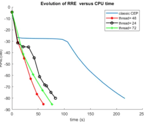
Figure 1. Performance vs CPU time for different number (thread) of candidates created in parallel
In Fig. 1 and Tab. I, we clearly observe that the application of a parallel strategy on the CEP algorithm allows to reduce the computation time. Moreover, all variants of the algorithm were able to reach the true solution as it appears on the Figure 3. The best choice among the different values of thread seems to be here thread = 48 for 96 available processors.
The lasting time between two records becomes shorter when the number of thread is decreasing and inversely. It makes
Table I
COMPARISON OF THE MEAN TIME CONSUMED DURING40000ITERATIONS AND MEAN NUMBER OF ACCEPTATIONS BY ITERATION VERSUS THE
NUMBER OF THREADS CREATED IN THE PARALLEL SECTION
Number of threads 24 48 72 Mean time during 40 000 iterations 9.24s 12.05s 19.11s Mean number of acceptations 17.88% 19.58% 22.49%
sense because thread cost function values for the new created candidates are computed at each iteration.
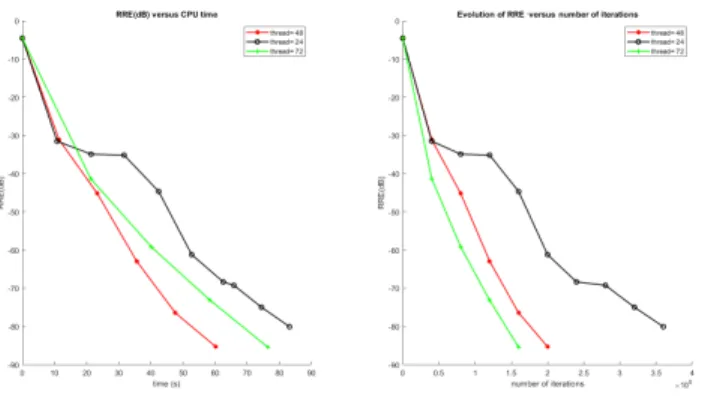
Figure 2. Impact of the number of new created candidates thread on the perf.
As illustrated on Fig. 2, the parallel strategy version with thread= 72 leads to convergence in less iterations. Indeed, the more created threads there are, the less iterations to achieve the converge are required. However, this version of the algorithm is not the fastest since each iteration takes much more time to be completed. As a conclusion, there is a compromise to find between the time taken by each iteration and the total number of iterations required to reach the stopping criteria but with this kind of stochastic algorithm it remains obviously advantageous to opt for a parallel strategy.
Figure 3. Comparison of the emission and excitation spectra estimated with the different variants of the algorithm superimposed with the ground truth spectra.
VI. CONCLUSION& PERSPECTIVES
The parallel strategy for the CEP algorithm used to solve the CP decomposition problem is less time consuming than the
standard version of the CEP algorithm (about 3,6 times) while the same accuracy can be reached. However, we have shown that the number thread of new candidates must be carefully chosen. In [8], a locally optimal step size strategy has been developed on a random variable to reduce the rejection rate in the original version of the CEP algorithm. Our aim will be now to use both this parallel strategy and the locally optimal step size strategy. New candidates will be created by calculating and applying this “optimal step size” for different variables picked in parallel. Finally, many other parallel strategies could be considered, among which are the application of all the accepted moves on the previous candidate, or the use of the second best move in the previous iteration at the local search stage in the parallel region to avoid the loss of important acceptances.
REFERENCES
[1] T. G. Kolda and B. W. Bader, “Tensor decompositions and applications”, SIAM Review, 51:3, pp. 455-500, 2009.
[2] F. L. Hitchcock, “The expression of a tensor or a polyadic as a sum of products”, Journal of Mathematics and Physics, 6, 1927.
[3] A. Cichocki, R. Zdunek, A. H. Phan, and S. I. Amari, “Nonnegative matrix and tensor factorizations: applications to exploratory multi-way data analysis and blind source separation”. Wiley Publishing, 2009. [4] X. T. Vu, C. Chaux, N. Thirion-Moreau, S. Maire and E. M. Carstea
“A new penalized nonnegative third order tensor decomposition using a block coordinate proximal gradient approach: application to 3D fluorescence spectroscopy” in Journal of Chemometrics, Wiley & Sons, special issue on penalty methods, Vol. 3, CEM 31.1, March 2017. [5] N. Vervliet, L. De Lathauwer, “A randomized block sampling approach
to canonical polyadic decomposition of large-scale tensors”. In IEEE Journal of Selected Topics in Signal Processing 10.2, pp. 284–295, 2016. [6] X. T. Vu, S. Maire, C. Chaux and N. Thirion-Moreau, “A new stochastic optimization algorithm to decompose large nonnegative tensors”, in IEEE Signal Processing Letters, vol. 22, no. 10, pp. 1713-1717, Oct. 2015.
[7] P. Moscato, “On evolution, search, optimization, genetic algorithms and martial arts - Towards memetic algorithms”. Caltech Concurrent Computation Program, Report. 826, 1989.
[8] S. Maire, X. Vu, Caroline Chaux, C. Prissette, N. Thirion-Moreau. “Decomposition of large nonnegative tensors using memetic algorithms with application to environmental data analysis”. 2019. hal-02389879 [9] J. R. Lakowicz, “Principles of fluorescence spectroscopy”, 3rd edition
Springer ISBN: 978-0-387-31278-1 Hardcover, 2006.
[10] J.P. Royer, N Thirion-Moreau, P. Comon, R. Redon and S. Mounier “A regularized nonnegative canonical polyadic decomposition algo-rithm with preprocessing for 3D fluorescence spectroscopy”, Journal of Chemometrics 29 (4), 253-265, March 2015
[11] J.-P. Royer, N. Thirion-Moreau, P. Comon, “Nonnegative 3-way tensor factorization taking into account possible missing data”, in Proc. EU-SIPCO, pp. 71-75, Bucharest, Romania, August 2012.
[12] G. Tomasi, R. Bro, “PARAFAC and missing values”, Chemometrics and Intelligent Laboratory Systems, Vol. 75, Issue 2, pp. 163-180, 2005. [13] L. Cannelli, F. Facchinei, V. Kungurtsev, and G. Scutari. “Asynchronous
parallel algorithms for nonconvex big-data optimization: model and convergence”. ArXiv, abs/1607.04818. 2016.
[14] A. P. Liavas and N. D. Sidiropoulos, “Parallel algorithms for constrained tensor factorization via alternating direction method of multipliers”, in IEEE Trans. on Signal Proc., vol. 63, no. 20, pp. 5450-5463, Oct. 2015. [15] N. D. Sidiropoulos, E. E. Papalexakis and C. Faloutsos, “A parallel algorithm for big tensor decomposition using randomly compressed cubes (PARACOMP)”, IEEE International Conference on Acoustics, Speech and Signal Processing (ICASSP), Florence, 2014, pp. 1-5, 2014. [16] J. Tang, M. H. Lim, Y. S. Ong, “Diversity-adaptive parallel memetic algorithm for solving large scale combinatorial optimization problems -Soft Computing”, Springer, 2007.