Introduction to Linear Data Analysis

ADE-4

Introduction to Linear Data

Analysis

Abstract

This volume describes the main features of the mathematical model associated with the linear multivariate methods incorporated into ADE-4 software. The main characteristics of statistical computation for one-table analysis are incorporated. ADE-4 is a data analysis package designed for descriptive statistics, which is useful for large data sets to investigate the structure or the organisation of data. Several illustrations of that volume are part of papers from Chessel & Thioulouse (1990, Auto-modélisation en analyse des données. In : Modélisation confluent des sciences. Brissaud, M., Forsé, M. & Zighed, A., Eds., Editions du CNRS. Paris. 71-86), Thioulouse et al. (1991, Graphical techniques for multidimensional data analysis. In :

Applied Multivariate Analysis in SAR and Environmental Studies. Devillers, J. & Karcher, W.,

Eds., Kluwer Academic Publishers. 153-205), Dolédec & Chessel (1991, Recent developments in linear ordination methods for environmental sciences. Advances in Ecology, India : 1, 133-155), and Chevenet et al. (1994, A fuzzy coding approach for the analysis of long-term ecological data. Freshwater Biology : 31, 295-309).

Contents

1 - Factorial maps ...2

1.1 - Coordinate system...2

1.2 - Construction of an orthonormal coordinate system...4

1.3 - Change of basis ...6

1.4 - Projection onto a plane...8

2 - Data modelling...10

2.1 - Data, models and residuals... 10

2.2 - Implicit models vs. trivial models ...14

3 - Coding ...16

3.1 - Observed data...17

3.2 - Qualitative models... 17

3.3 - Neighbourhood structures ...19

4 - Statistical modules...20

4.1 - Mathematical basis of the computation... 20

4.2 - Statistical triplet: various alternatives ...22

4.3 - Interpreting data analysis ...28

Références ...31

1 - Factorial maps

1.1 - Coordinate system

Let x and y be a pair of numbers. Making a Cartesian diagram consists of: (i) drawing two perpendicular straight lines,

(ii) selecting units,

(iii) placing the point using its x-axis and y-axis coordinates.

A (-1,2) U U U U -1 2 -1 -1 2 2 A (-1,2) (-1,2) A

Figure 1 Cartesian diagram.

One may use two non perpendicular axes and use various units on each axis. In Figure 1, only the first graphic (on the left) is a true Euclidean diagram.

U x

y T

Figure 2 Euclidean diagram (on the right) and corresponding Cartesian diagram (on the left).

Considering any concrete 3D object (e.g., a chapel in Fig. 2), it may be very useful to have a list of characteristic points of the object. The Cartesian diagram using these points allows to interpret the resulting representation of the object. Obviously, the change from the 3D object to the 2D Cartesian diagram involves distortions. Among the various ways to make this change, there is only one, which uses linear algebra, that permits to draw Cartesian diagrams of a more than three dimensions conceptual object. The Euclidean representation is a basic tool for graphical display in the exploratory data analysis.

Consequently, an Euclidean diagram results of any Cartesian diagram of several points by using the vector space properties.

Let _Rn(n=1,2,…,) be the set of all n-tuples of real numbers. Let Ε =R3. Let M=(x,y,z) be an element of E. The three following elements of E are essential as they form a canonical basis:

I=(1,0,0) J=(0,1,0) K=(0,0,1)

These three vectors are linearly independent. 0 = (0,0,0) is the null vector. To every pair, M and N, of vectors in E there corresponds a vector M+N, called the sum of M and N in the following way:

To every pair, a and M, where a is a scalar (a real number) and M is a vector in E, there corresponds a vector aM in E called the product of a and M as follows:

aM=a(x,y,z)=(ax,ay,az)

In the so-called vector space E, all the following properties are satisfied:

M+(N+P)=(M+N)+P M+(−M)=(x, y ,z)+(−x,−y,−z)=0 a(bM)=(ab)M a(M+N)=aM+aN M+0=M+(0 ,0 , 0)=M M+N=N+M (a+b )M=aM+bM 1 M=M

The vector M= (x,y,z) may be written in the following way:

M=xI+yJ+zK

Hence, M is a linear combination of the vectors I, J, and K using x,y and z coefficients. These x,y and z numbers are the coordinates or components of M in the canonical coordinate system. We must now distinguished the element M defined by (x,y,z) from a table containing three rows and one column as follows:

M= x y z           and the corresponding transposed matrix:

M'=[x y z]

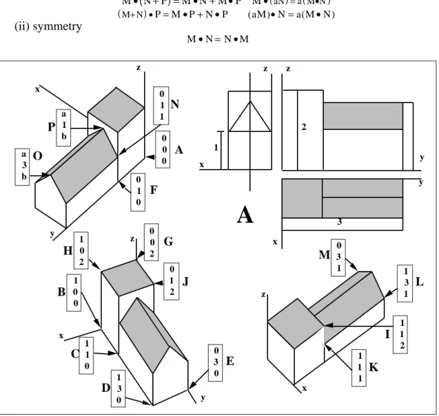
because M = (x,y,z) designates the vector and the corresponding table designates one of its possible representation. The following set of 16 elements in E is necessary to make Euclidean diagrams of the chapel as illustrated in Fig. 3:

A B C D E F G H I J K L M N O P -0 1 1 1 -0 -0 -0 1 1 -0 1 1 -0 -0 a a 0 0 1 3 3 1 0 0 1 1 1 3 3 1 3 1 0 0 0 0 0 0 2 2 2 2 1 1 1 1 b b with a = 1/2 and b = 3

This example aims to demonstrate the major purpose of a model as stated by Legay (1973)1_.

The addition of two points of any concrete object does not make any sense for the concrete object. Hence, the only available property of a model is its usefulness, i.e. what one can make with that model (in our example, the model allows to draw an image of the chapel). Adding points has no concrete meaning, but considering points as linear combinations may be very efficient to have a representation of the concrete object.

1.2 - Construction of an orthonormal coordinate system

To every pair M and N of vectors in E there corresponds a real number as follows: M•M=(x,y,z)•(t,u,v)=xt+yu+zv

This linear functional is called scalar product and has two properties: (i) bilinear form

M•(N+P)=M•N+M•P M•( )aN =a M( •N) M+N ( )•P=M•P+N•P (aM)•N=a(M•N) (ii) symmetry M•N=N•M 2 3 1 x z x y z x y z x y z x y z

A

Figure 3 Sixteen points of E are characteristic of a chapel. A is the plane of the front, profile and top views of the chapel. In that case, the 16 points are positioned using three Euclidean diagrams. The grey areas permits to interpret (or to visualise) the chapel. However, the grey areas as well as the hidden areas do not belong to the model and are displayed to facilitate the interpretation of the concrete object.

Furthermore, if M = N, the scalar product has a positive or null value for the vector (0,0,0):

M•M=(x,y,z)•(x,y,z) M•M=x2+y2+z2

The scalar product is said strictly positive. Let M•M=||M||2. The number ||M|| is called the norm or the length of the vector M. Let ||I||=||J||=||K||=1. The vectors I, J, and K are called unitary vectors.

A very useful property (with important arithmetic, geometric and analytic consequences) is called Cauchy-Schwarz's inequality. For every pair of vectors M et N:

||M||2||N||2≥(M•N)2 Furthermore, the equation:

implies that the trinome has a negative or null value proving the Schwarz's inequality. This allows the angle to be defined between vector M and N as equal to α (with

0<α≤Π) so that:

cos =M•N/||M||||N|| Hence, for two orthogonal vectors:

M•N= 0 since in that case:

= Π/2.

Consequently, three orthogonal-in-pair vectors (I,J,K) in E form an orthogonal coordinate system. If (I,J,K) are unitary vectors as follows:

I=(1,0,0) J=(0,1,0) K=(0,0,1)

they form an orthonormal coordinate system. Hence, the vectors (I,J,K) form an orthonormal coordinate system verifying:

I•J=I•K=J•K=0

As a result, making Euclidean representations amounts to finding an orthonormal coordinate system. There are many ways to reach such an objective. Data analysis first relies on the spectral decomposition of a symmetric linear transformation. We are giving a simple concrete procedure in Fig. 4 to illustrate the above remarks. Any point of a sphere centred at the origin, with radius equal to R, may be located by only two angles (α and β). Let R = 1, this results in a unitary vector as follows:

U=(cos cos ,cos sin ,sin ) Moreover, the vector:

V=(−sin ,cos ,0) is a unitary vector orthogonal to U. The vector:

W=(−cos sin ,−sin sin ,cos )

is a unitary vector orthogonal to U and V. Vectors U, V, and W form an orthonormal coordinate system, which is said associated to (α,β) angles.

The following table is a square matrix that contains the respective coordinates of U, V, and W (as columns) in the canonical coordinate system:

Mat(U ,V, W)=H=

cos cos −sin −cos sin cos sin cos −sin sin

sin 0 cos          

1.3 - Change of basis

The vector M=(x,y,z) may be written in the following way: M=xI+yJ+zK

Furthermore, the linear combinations may be calculated as follows: cos cos U−sin V−cos sin W=I

cos sin U+cos V−sin sin W=J sin U+0V+cos W=K ( U , K )Plan 60° 5° 2 3 4 5 0°,30° 0°,60° 60° 135° 60° 25° 60° 45° 60° 60° 0°,0° 9 1 x y z P 60° 85° 6 8 7 (I,J) Plan

Figure 4 Diagram of 9 points belonging to a sphere centred at the origin. Two angles ( and ) are sufficient to locate a point. The Euclidean representations of the chapel associated to each point, i.e. as if the observer viewed the chapel from that point, are represented in the 9 inset windows that include the corresponding angle measurements. (From 2)

Consequently, M may be written as a linear combination of U, V, and W: M=(xcos cos +ycos sin +zsin )U+(−xsin +ycos +z0)V

+(−xcos sin −ysin sin +zcos )W

These complex calculations are managed by means of matrix calculation. Consequently, the user is supposed to be sufficiently informed about elementary matrix calculations. Let: M=aU+bV+cW then: a b c           =

cos cos −sin −cos sin cos sin cos −sin sin

sin 0 cos           x y z          

The vector M may be written with both the following equations respectively in the canonical coordinate system and in the basis (U,V,W):

M=xI+yJ+zK with M₁= x y z           and M=aU+bV+cW with M2= a b c           (1) Using the matrix notation, one may write:

M₂=H'M_{1 and} M₁=HM₂

H' is the transposed matrix of H, which is an orthonormal matrix: H'H =HH'=I₃

with I3 being the identity matrix that has 3 rows and 3 columns. Consequently, the permanent vector M (in R3) can be expressed by the matrices noted M1 and M2 as supported by equations (1). Therefore, the matrix calculation is a convenient tool that facilitates a change of basis. Note that the same matrix calculations may have a different meaning when used in another context. For instance, let O be a point defined in Fig. 3 as follows:

O = (1/2, 3, 3 )

and let us consider the change of basis associated to α = 30° and β = 60° angles. Matrix H is equal to: H= 0.433 −0.5 −0.75 0.25 0.866 −0.433 0.866 0 0.5           The transposed matrix H' is equal to:

H'= 0.433 0.25 −0.866 −0.5 0.866 0 −0.75 −0.433 0.5           The change of basis from (I,J,K) to (U,V,W) is as follows:

M₂=H' M₁= 0.433 0.25 −0.866 −0.5 0.866 0 −0.75 −0.433 0.5           0.5 3 1.732           = 2.467 2.348 −0.808          

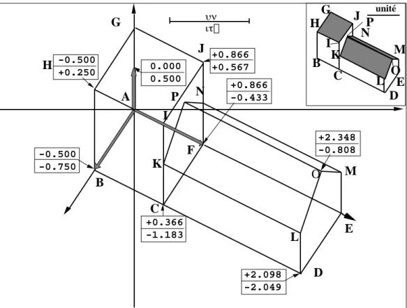
Consequently, any point may have its own coordinates in the (U,V,W) coordinate system. Two coordinates may be selected for a Cartesian diagram e.g., the second and the third coordinates equal to (2.348, -0.808). Thereby, the 16 points already used in Fig. 3 are situated using an ordinary coordinate system (Fig. 5), i.e. two perpendicular axes and one length unit.

This results in an Euclidean diagram associated to (α, β) angles. Furthermore, the vector of (I,J,K) basis standing for the points of coordinates (1,0,0), (0,1,0) and (0,0,1) are represented by the same way. One major characteristic of the Euclidean approach lies in that the resulting representation is a new object from which one may draw a new representation, thus referring to the projection theorem.

B 0.000 0.500 +2.098 -2.049 +0.866 +0.567 unité -0.500 -0.750 A C D E F G H I J K L M N P B C D E G H I J K L M N O P +0.366 -1.183 -0.500 +0.250 +0.866 -0.433 +2.348 -0.808

Figure 5 Cartesian diagram of the 16 points of the chapel resulting from a change of basis. The vectors of the canonical coordinate system are represented by a thick grey line. The insert at the upper right hand corner contains the interpretation of the diagram with grey and hidden areas. Data analysis follows the same procedure and displays the methods of representation on one hand and interpretation on another hand.

1.4 - Projection onto a plane

In a vector space, the addition and multiplication by a real number represent major operations that define linear combinations. A Euclidean space (or inner product space), is a vector space provided with an inner product. Let f be a linear transformation associating a vector M of a Euclidean space to a vector T = f(M) of the same Euclidean space. f will be considered as an automorphism, i.e., an isomorphism of a vector space with itself, if the following algebraic operations are true for every pair of vectors M and N in E and for every a in R:

f(M+N)=f(M)+f(N) f(aM)=af(M)

Rotations, symmetry and projections are linear transformations. A linear transformation (automorphism) f is perfectly defined for the values of the coordinate system vectors:

f(M)=f(xI+yJ+zK)=xf(I)+yf(J)+zf(K)

If the vectors f(I), f(J) et f(K) are defined in another coordinate system (U,V,W) using the matrix notation as follows:

F= a₁₁ a₁₂ a₁₃ a₂₁ a₂₂ a₂₃ a₃₁ a₃₂ a₃₃           that corresponds to the more complex notation:

f(I)=a₁₁U+a₂₁V+a₃₁W f(J)=a₁₂U+a₂₂V+a₃₂W f(K)=a₃₁U+a₃₂V+a₃₃W

then T = f(M) = aU+bV+cW results in the following matrix operation: a b c           = a₁₁ a₁₂ a₁₃ a₂₁ a₂₂ a₂₃ a₃₁ a₃₂ a₃₃           x y z          

T is defined in the (U,V,W) coordinate system and M is defined in the (I,J,K) coordinate system. Matrix F is the so-called f linear transformation matrix from the source coordinate system b₁=(I,J,K) to the destination coordinate system b₂=(U,V,W). Consequently, in the previous paragraph, H' was the matrix of the identity linear transformation that associates M to M from b₁ to b₂, whereas H was the matrix of the identity linear transformation that associates M to M from b₂ to b₁. Change of basis, amount to the use of the simple identity linear transformation.

Note that the matrix of identity is the identity matrix only if the two bases are similar.

Let now f be a linear transformation that associates T = f(m) to m defined in b₂ as follows:

M=aU+bV+cW

and T=f(M)= 0U+bV+cW=bV +cW

Such a linear transformation simply cancels the first coordinates in b₂. A new execution has no effect:

f(f(M)) = f(M)

We say f is a projection operator. Furthermore, the scalar product between the vector f(M) and the vector M - f(M) is equal to 0 since the coordinate system is orthornormal:

(bV+cW)•(aU+bV+cW−bV−cW)=ab(U•V)+ac(U•W)=0

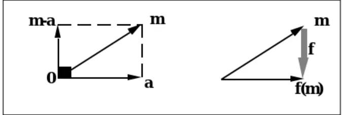
Furthermore, in the plane defined by M and f(M), we have the relation illustrated in Fig. 6. m a m-a 0 m f(m) f

Figure 6 Linear projection transformation.

As a result, we say f is an orthogonal projection operator. All the representations resulting from the projection operator are linear combination of V and W (bV+cW), i.e. they belong to the plane defined by V and W.

Moreover, all the vectors of the plane are their own images. Hence, f is the orthogonal projection operator on plane (V,W). As a result, the Euclidean diagram of an object is nothing but a representation of the object on the plane on which it is projected (when this plane is the sheet of paper). The projected points themselves form a new object, which is a flat object that may be visualised at any angle. An example of such an operation is given in Fig. 7. Each point of the chapel (A,B, ..., P) is projected onto plane

(V,W) using (25°,60°) angles. Then, the chapel and the projected chapel are represented by means of a projection on plane (V,W) using (135°,45°) angles. As a result, the projection of an object associated with a change of basis makes a convenient geometric initiation to data reconstitution (modelling).

Figure 7 One Euclidean representation of the object characterised by 16 points (A,B, ..., P) viewed with (135°, 45°) angles and one Euclidean representation (a,b, ..., p) viewed with (25°, 60°) angles, i.e. projection of the 16 points on the plane (grey area) perpendicular to (25°, 60°) angles. The projection involves distortions in the resulting graphics because the multiplication of two projection operators is generally not equal to one projection operator. In the insert, the grey tint plane is brought back onto the sheet of paper resulting in the Euclidean representation associated to (25°,60°) angles. This representation is a new object having its own representation. This operation, resulting in the representation of a representation, is essential for data reconstitution.

2 - Data modelling

Pearson (1901)3 _{first searched for a projected plane that minimises the residual sum of} squares. This option made the basis of the so-called factorial analysis strategy. Furthermore, substituting predicted data (more simple) to the observed one was the first objective of multidimensional statistics and resulted in simulating procedures (data modelling theory4_{). The resulting model considered as an instrument is an exploratory} tool of data and consequently data analysis is a modelling technique. When accepted, that basic notion5 _{invalidates every quarrel between trends in statistics. Its own identity} and its interest, lies in that the properties of the model arise from the data themselves6_.

2.1 - Data, models and residuals

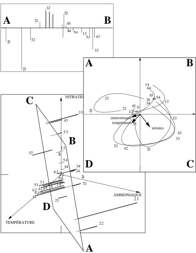
The principle of auto modelling is illustrated in Fig. 8. A number of p variables are measured on n individuals (sampling units), resulting in n points M_i (1≤i≤n) in Rp. Each point is projected onto a subspace (reduced dimensions) resulting in the following decomposition:

using x_ij as a measurement of the jth variable on the ith individual (sampling unit), m_ij as the corresponding coordinate of the projected point and rij as the difference between x_ij andm_ij.

A

B

C

D

A

B

D

A

B

C

Figure 8 Projection (geometric operation) and modelling (numerical operation) have the same nature. In this example, three variables were sampled on four occasions at six sites resulting in 24 points of R3_.

Plane (A, B, C, D) has the maximum inertia (variability). In front view, (A, B, C, D) is a factorial map. In profile view, one may visualise the residuals of the projection. The observed data and the resulting model are points in R3_{. The residuals are vectors (thick lines for projections). Hence, maximising variability on}

As a result, classical data analysis methods differ by three ways: (i) the weight of points;

(ii) the metrics (how the distances are measured between individuals or sampling units) used in Rp;

and (iii) the initial transformation of data (e.g., centring, normalising, variable changes).

A further diagonalization generates an orthonormal coordinate system (axes). The change into that basis generates Euclidean representation (factorial maps). The return back to the canonical coordinate system after projection results in model and residual displays. Borne with the inferential statistics7_{, this geometric approach was clearly} stated by Bartlett (1934)8_.

These authors considered at first p points in Rnwhereas Pearson (op. cit.) considered

n points in Rp

. The duality diagram of French tradition has made a synthesis of the two statements. This geometric approach, we say without explicit hypothesis, confers the same status to the model and to the residuals.

Hence, let mk(i,j) be the jth coordinate in the canonical coordinate system of the projection of the kth principal axis of the ith point, we have the following relation:

x_ij= m_k( )i,j k=1,r₀

∑

∑

∑

which corresponds to the following equation:

data = model + ? + residuals

The question mark (?) may be integrated either into the model or into the residuals. Inertia analysis checks this plasticity resulting in a better data scrutiny but also involving difficulties. Such a property can be used in principal components analysis (PCA) as illustrated in Fig. 9.

Let xij be the normalised value of the jth variable and let Mi (1≤i≤n) form the chronological sampling. The model using the first principal axis is as follows:

x_ij=a_ib_j+r_ij

It permits to place on each observed data curve, the unique curve (α₁, ..., α_n) apart from scale coefficient β_j. The residual sum of squares is minimum. Several axes may be progressively incorporated as illustrated in Fig. 10.

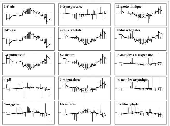
1-t° air 2-t° eau 3-conductivité 4-pH 5-oxygène 10-sulfates 9-magnesium 8-calcium 15-chlorophyle 14-matière organique 13-matière en suspension 12-bicarbonates 7-dureté totale

6-transparence 11-azote nitrique

Figure 9 Modelling data after principal components analysis (PCA). One can view simultaneously the chronically sampled data (bars) and the best model defined by the first axis of PCA (thick lines). This model is adjusted to a number of variables (scales common to all windows, [0,400] days for x-axis, and [-3,+3] normalised values as y-axis).

6-transparence 14-mop 1 1+2 1+2+3 1+2+3+4 1 1+2 1+2+3 1+2+3+4

Figure 10 Graphical representation of a PCA. Reconstitution of variables 6 (transparency) and 14 (particulate organic matter) by means of the four first axes. Data are represented by a thin line. Models are represented by a thick line. The progress made using graphical methods involves slight modifications in statistics, especially for the statistical methods that allow to interpret numerical information.

2.2 - Implicit models vs. trivial models

In practise, data analysis is considered as data modelling only by mathematicians, whom are not the majority among program users. This involves some confusion because numerical data often embody obvious characteristics (e.g., temperature is high in summer and low in winter). Such trivial effects may be eliminated. For a table of n rows and p columns, let t be the trivial effect as follows:

x_ij=t_ij+(x_ij−t_ij) with

____________________________________________________________________________________

tij estimate associated method

____________________________________________________________________________________

tij = 0 no non centred PCA

tij = constant x global mean only one centring PCA

tij = ai x i mean by row centred by row PCA or Q mode

tij = bj x j mean by column centred by column PCA or R mode

tij = ai + bj x i+x j−x double centred PCA

tij = aibj x ix j/ x COA (non uniform weights)

tij = aibj using diagonalization non centred PCA with deletion of

the first axis (uniform weight)

____________________________________________________________________________________ The combination between the part inherent to data (trivial effect) and the part selected from the analysis (modelling) may generate the following values:

x_ij= a_ij

k=1,m

∑

xij = µ + ρ_{i +} γ_{i + Qi}γ_{j + rij} from the first axis of a double centred PCA10_.

As a consequence, for several users, multivariate methods can show evidence because the same technique may either eliminate a trivial effect (residual study) or by contrast take such a trivial effect into consideration (to simplify the data). Generally, there are not many options in data analysis programs already diffused. Moreover, these options are often implicit. For example, a COA program does not ask any question and imposed a multiplicative double centring without notice. The illustration in Figure 1.11 demonstrates that doing so an essential part of the information may be removed . It is also true that open programs (with many options) makes the user doubt about the relevant selection. These remarks about trivial effects allow us to consider multivariate methods processed after the modelling11_.

Furthermore, one may generalise the processes in considering the parametric model m of a given table (row modelling, column modelling or global modelling) and in analysing the table having the following y_ij values:

y_ij =x_ij−m_ij

Such an analysis reveals a second type of parameters of the model according to the residuals generated by the model.

This strategy was initiated by Escofier (1983a)12_{, (1984)}13_{. Furthermore, if the} model is derived from a Euclidean approach, this strategy is connected to instrumental variable analyses14,15_{. Hence, it is possible:}

(i) to generate numerical simulation acting as models. Developments in multiple table analysis16 _{allow to take into consideration a number of dimensions as follows:}

x_ijk= _{il jm}

l,m,n

∑

(ii) to study the residual structure from a simple model (trivial structure) or a more sophisticated one (functional structure).

(iii) to initiate numerical simulation followed by the modelling of residuals: x_ij= _j( _ky_jik k=1,r_j

∑

∑

as in PCA on instrumental variables viewed as a simultaneous multiple regression.

zone à Truite 13 2 -1.5 -1.5 2 a b c d e f g hi j k l _m n o p q r s t u v w x y z + 7 1 2 3 4₆ 5 8 9 10 11 14 15 16 17 18 19 20 21 22 23 25₂₄ 26 27 28 29 30 12

station vide stations polluées

BAS zone à Ombre zone à Barbeau zone à Brème F1 x F2 espèces 15 -7 -7 15 F1 x F2 relevés 45 Valeurs propres HAUT

Acp centrée

Afc

Figure 11 Example of implicit modelling in multivariate analysis programs. Twenty seven fish species (a,b, ..., +) were sampled on the Doubs river in 35 locations (01, ..., 35). The table was processed with PCA and with COA. The centred PCA of the table takes into consideration the richness and the abundance of the fish populations from the upper reaches to the downstream reaches. These two parameters decrease abruptly between station 27 and 28 because of a pollution effect. The river has its quality restored from stations 30 to 35. The pollution effect is automatically removed in correspondence analysis (COA) by the double centring. This example demonstrates that using the same technique it is possible to remove either a sampling device (e.g., heterogeneity in sampling intensity resulting in abundance variations among samples) or a very important part of the data (e.g., environmental perturbation resulting in abundance variations among samples). Data from Verneaux (1973) 17 (modified from Dolédec & Chessel (1991)18). Fish species are identified as follows: a:

Sculpin, b: Trout, c: Minnow, d: Stone Loach, e: Grayling, f: Blageon, g: Nase, h: Southwest European Nase, i: Dace, j: Chub, k: Barbel, l: Stream bleak, m: Gudjeon, n: Pike, o: Perch, p: Bitterling, q: Pumpkinseed, r: Rudd, s: Carp, t: Tench, u: Bream , v: Black Bullhead, w: Ruff, x: Roach, y: White Bream, z: Bleak, +: Eel.

Between-groups and within-groups analyses19,20 _{and the analyses of projected} subspaces such as partial canonical correspondence analysis21 _{and internal} correspondence analysis22 _{rely on this approach.}

3 - Coding

Using a classical program, one "cannot see the forest for the trees". In another way, we believe that data analysis is a methodological tool enabling various practises. After, the use of scores for factorial maps and data reconstitution, the third major idea is coding.

Geometrically, we use vectors, i.e. points in Rk_{. Let y be a vector expressed in the} canonical coordinate system or in another coordinate system, i.e. let y be the list of its coordinates y(1), y(2), ..., y(k). These k coordinates are k numbers or a code using k elements. One may use this code as any other measurement series, e.g., for making histograms, curves, or any representation, for calculating the mean. Hence, to select one representation among the various possibilities, one must define optimal properties of a given representation. Here are three examples.

3.1 - Observed data

One may transform quantitative variables into categories by grouping the sampling units. The inverse transformation is also possible by calculating a numerical code for categories. Data analysis makes optimal codes by maximising quadratic forms. For example, the codes of rows and columns of a contingency table maximising the correlation are the result of the first scores in correspondence analysis23_.

2 3 4 5 6 7 8 0 1 1 . 5 3 . 5 5 . 5 7 . 5 9 . 5 1 1 . 5 1 3 . 5

A

B

Figure 12 The age (from 1 year old to 8 years old and upper) and the number of kitten produced for the whole year, 1 or 2 (1.5), 3 or 4 (3.5), ..., 13 or 14 (13.5) were recorder for 350 cat females. The elementary bivariate plot (A: square surfaces proportional to the number of observations), the regression curve (A: correlation ratio equal to 0.089), and the regression straight line (A: R2 _{= 0.073) make the}

descriptive statistics giving information about the relationship between the age and the number of kitten. COA of the contingency table results in recoding rows and columns of the table by maximising the observed correlation so as to make a linear connection (B) between row codes and column codes24. Five categories of ages (1, 2, 3, 4 to 6, 7 and upper) and two categories of fertility (1 to 6, 7 to 14) are displayed. The correlation ratio, R2 _{and the first eigenvalue is equal to 0.114. As a result, coding}

elements using Euclidean methods is a way to take into consideration non linear relationships. Data from Legay and Pontier (1985)25.

Thereby, the scores resulting from a multivariate analysis may be better for interpretation than the observed data, i.e. the exchange from a quantitative measurement

to a categorical measurement and from a categorical measurement to a numerical code give much more experimental meaning to the studied data, as shown in Fig. 12.

-2.0 -4.8 +2.8 +5.3 F1 F2 25 12 14 15 1 27 5 9 20 37 21 24 23 13 34 31 18 22 7 26 40 39 4 6 8 17 16 10 36 19 8 10 44 49 50 3 4 5 13 2 51 6 11 1 46 ₄₈ 12 45 42 38 23 21 28 27 26 43 35 31 CENTRE VILLE QUARTIERS BANLIEUES RURAL OUVERT RURAL FERMÉ

Figure 13 Quantitative modelling of an ecological structure (ecotone). Data from Tatibouet, F., Chessel, D., Broyer, J. & Lebreton, J.D. (1980) Etude des peuplements d'oiseaux nicheurs de la zone urbaine de Lyon. Rapport final du Contrat Ecologie urbaine n° 237-01-78-00314. Ministère de l'Environnement. 106-156..

By the way, multiple correspondence analysis (MCA) (see a synthesis in Tenenhaus & Young (1985)26_{) and derived analyses are supported by such a principle.}

3.2 - Qualitative models

One major characteristic of ecological systems (space dispersion, species association, species-environment relationships) lies in the diversity corresponding to the great variety of living organisms. Such a variety suggests that we need some freedom for modelling.

Any unexpected representation of an ecological structure, i.e., a representation that does not belong to a pre-established kind must be integrated into the modelling. Euclidean methodology is one way to find such discursive models. The above idea is at the basis of biometry27_{, and at the basis of data analysis}28_.

An example is given in Fig. 13. Forty bird species (listed on the right) were counted in 51 samples by means of listening points. These samples were distributed on a transect beginning in a rural area, crossing district boroughs, reaching the town centre, and further extending to open rural area located at the south of the town. Each species-sample correspondences (different from 0) is placed on a factorial map by the corresponding sum of COA row and column scores, total variability being equal to 129_.

Each species is represented by an inertia ellipse standing for its habitat amplitude (top of Fig. 13). Each sample is treated in the same way by expressing taxa diversity found in samples (bottom of Fig. 13). The centres of ellipses are nothing but the classical factorial map. Axis 1 is interpreted as a gradient from the town to the rural area and axis 2 discriminates the open and close area that greatly influence bird distribution. Comparing the two maps allows a statement of the hardly quantifiable ecotone concept,. As a result, there are two kinds of samples (urban/rural) and a marked boundary between the groups of samples. That interface is at the mean dispersion of a number of species. Consequently, one may found the greatest diversity at the interface. Such a practise considering COA as a canonical analysis is not widespread.

3.3 - Neighbourhood structures

Lebart (1969)30_{, (1984)}31 _{initiated neighbourhood graphs in data analysis. The} diagonalization of an automorphism (Fig. 14) generates reference codes (eigenvectors) only depending on the selected relationship.

These scores can be used as independent variables for multiple regression. They may be called endo-models in that they are connected to an automorphisms and stemming from endogenous process.

In conclusion, inertia and projection computation, data reconstitution and auto modelling, and coding result from the same theorem: any symmetric matrix can define an orthonormal basis of eigenvectors. ADE software incorporates interpretation aids for the three types of operation all belonging to the eigenvalue analysis (linear methods). Among the ordination methods, linear methods are the only ones that can be mathematically described. Consequently, they are not depending on the software support.

4 - Statistical modules

We will not go further into mathematical modelling, but some remarks may help the user in understanding the calculations made with ADE. The duality diagram32 _was introduced in ecology by Escoufier (1987)33 _{to adapt mathematical abstractions to} concrete situations. As stated by Ramsay (1982)34 _{the duality diagram "can be} considered a fundamental algebraic advance over matrix analysis, and it is to be hoped that it will become a standard part of statistical language". This approach was one way to synthesise the first work made in ecology by Noy-Meir (1973)35_{, the practical} approach of Laurec (1979)36 _{and the theoretical introduction of Laurec et al. (1979)}37_. Furthermore, the duality diagram is receiving increasing use e.g., in ecology by Pialot (1985)38_{, in chimiometry by Sanlaville-Boisson (1989)}39_{, in evolutionary biology by} Yoccoz (1988)40_.

Figure 14 Numerical scores associated to a neighbour graph. Twenty-five points form a chessboard (5 rows and 5 columns). Two points are next if they follow each other on the same line or the same column (tower principle). M is the associated matrix (25 rows and 25 columns, using m(i,j) = 1, if i is next to j and m(i,j) = 0, if not). Dn is the diagonal matrix (25 rows and 25 columns) that contains the uniform weights. Dn* is the diagonal matrix that contains the sum of weights between two neighbour points. Dn*-MDn is the matrix of a Dn-symmetric projection operator which generates a Dn-orthonormal basis of eigenvectors. The coordinates of each eigenvector are represented by a square map (the 25th is constant) thus forming a finite list of reference figures as stated by orthogonal polynomes or Fourier series41.

The concrete element, we say a statistical triplet, is made by the data table and two weight matrices (Fig. 15). From a raw data table noted Z having n rows and p columns, let (X,D_p,D_n) be a statistical triplet composed of a table X having n rows and p columns, and two non negative norms D_p and D_n. A linear application is thus defined from the dual space of Rp toward Rn using the canonical basis and the two norms D_p and D_n. The positive numbers contained in D_{n form the diagonal of a square matrix} with n rows and n columns. The positive numbers contained in D_p form the diagonal of a square matrix with p rows and p columns.

Z raw data ROW COMPONENT SCORES COLUMN COMPONENT SCORES + EIGENVALUES INITIAL TRANSFORMATION columns 1 p rows 1 n C R ω 1 ω j ωp X π 1 π i π n Dp = 0 0 ω₁ ω_j ω p ω > 0 j Dn = 0 0 π₁ π i π n π > 0 i B = D X D X D BV = V and V V = I 1/2 1/2 n p t n t n C = X D V R = D V 1/2 t n -1/2 n 1/2 R = X D U C = D U 1/2 p -1/2 p 1/2 A = D X D X D A U = U and U U = I 1/2 1/2 n p p t p t Central procedure Central procedure Diagonalization λ _k + range X t ω 1 ω j ω _p π 1 π i πn n > p n < p 1 f 1 f 1 p 1 n ( X,Dp,Dn)

Figure 15 Central procedure of calculations in linear multivariate data analysis. The notations are consistent with the duality diagram. The option that the column number is larger than the row number (n<p) or vice versa (n>p) has no effect on the results (squares and circles stand for the row or column weight; Dn: row weight matrix; Dp: column weights matrix; X: transformed data table; Xt: X transposed

table; Ip and In are the identity matrices).

The following matrix endomorphisms (Escoufier's operators) are, respectively, symmetrical with respect to D_p and D_n.

XtD_nXD_{p (t for transposed) and} XD_pXtD_n

The associated orthonormal basis of eigenvectors defines the principal axes and the principal components. The quadratic forms defined, respectively, by:

Q u( )= XD_pu n D 2 with u p D 2 _{=1and S v( )= X}t D_nv p D 2 with v n D 2 ₌₁

are maximised under the constraint of orthogonality. Various graphical applications result from the above theorem among which the factorial map is well known as the

projection of the multidimensional space onto the optimal plane. Inertia calculations enable a control of the data deviation from the projection.

The central procedure of calculation is the so-called diagonalization (Fig. 15).

D_p 1 2 XtD_nXD_p 1 2 or D_n 1 2 XD_pXtD_n 1 2

The smaller dimension of the above matrices is really diagonalized. This results in an orthonormal basis to obtain the axes and the components of the eigenvectors from the multidimensional space of the n points of Rp and the p points of Rn. As a result, the factorial coordinates in one multidimensional space are proportional to the components of the eigenvectors in the other multidimensional space.

Further interpretation of multivariate analyses is usually based on such coordinates. For each axis, the coordinates are normalised by the square root of the corresponding eigenvalue. In other terms, the variance of the factorial coordinates of one axis is equal to the eigenvalue. The matrix that contains the coordinates of the n rows is deduced from the matrix that contains the coordinates of the p columns through the diagonalization procedure, using the transition formula:

R=XD_pC − 1 2 _{and C=} XtD_nR − 1 2

where R and C are the matrices of coordinates (rows and columns), and is the matrix of eigenvalues.

Furthermore, the initial table X may be presented as singular values as:

X=R − 1 2 1 2 − 1 2 Ct

Using this equation, the replacement of each point of table X by its projection onto subspaces generated by the k first eigenvectors results in data reconstitution (for an example in hydrobiology see Carrel et al., 198642_).

4.2 - Statistical triplet: Various alternatives

4.2.1 - Definition and analysis of a statistical triplet with ADE

Various procedures are available via ADE programs. These procedures, which all deal with the so-called statistical triplet, are incorporated in the option menu (Fig. 16). Every ADE program uses a binary file as input (e.g., Tab is a table with n rows and p columns). After processing by any multivariate technique, a "xx" character string designates the type of analysis (e.g., cp, cn, fc in Table 1) .

Figure 16 Popmenu button of the ADE•Base selection card (left) for making basic analysis and example of option of the PCA module (right).

These modules generates at least eight files as follows:

1- TAB.xxpa (parameters) ASCII file

2- TAB.xxma (margins) ASCII file

3- TAB.xxta (table) binary file

4- TAB.xxpl (row weights) binary file 5- TAB.xxpc (column weights) binary file 6- TAB.xxli (row scores) binary file 7- TAB.xxco (column scores) binary file 8- TAB.xxvp (eigenvalues) binary file

TAB.xxpa contains the number of rows (10 in the example below) and the number of columns (14) of the initial raw table, the number of axes stored (2) and the total inertia of the initial table (107.7) as follows:

10 14 2 +107.7

Table 1 Basic ADE modules for one-table analysis.

____________________________________________________________________________________

Modules options Title of the analysis

____________________________________________________________________________________

PCA Correlation matrix cn (normalised PCA)

PCA Covariance matrix cp (column centred PCA)

PCA After row % transformation row%.cp (PCA on percentage tables)

PCA Non centred nc (non centred PCA)

PCA Decentring x(i,j) - model(j) rl (decentred PCA using a reference point) PCA Decentring x(i,j) - model(i,j) nc (non centred PCA on the difference)

PCA Partial normed nm (within row group PCA alternative calculation) PCA Within group normalised nb (within row group PCA)

COA Correspondence analysis fc (COA)

COA Row weighted fc (modified COA)

COA Internal ww (within column and row group COA)

COA Decentred fr (decentred COA)

MCA Multiple correspondence analysis cm (COA of k categorical variables)

MCA Fuzzy correspondence analysis fl (alternative MCA of k fuzzy coded variables)

HTA No centring nc (non centred PCA)

HTA Overall centring cu (overall centred PCA)

HTA Column centring cp (column centred PCA)

HTA Row centring cl (row centred PCA)

HTA Double centring additive cc (double centred PCA) HTA Double centring multiplicative dm (double centred PCA)

____________________________________________________________________________________ TAB.xxma contains various information according to the analysed table (e.g., the number of rows and the number of columns, mean, variance or number of categories for one variable). This content is described in the program listing:

10 14 3.6 3.2 ………… 13.44

TAB.xxta is the transformed table having the same dimensions as the input data table (raw data). For example, running the PCA program with the Covariance matrix option creates a centred by columns table.

1 | 1.73 1.68 -0.02 0.35 0.66 -1.00 0.01 -1.00 -1.00 -1.00 2 | 1.73 2.39 1.94 1.13 -1.00 -1.00 -1.00 -1.00 -1.00 -1.00 ……… 14 | -1.00 -1.00 -1.00 -1.00 -1.00 0.35 -0.14 1.25 1.57 1.82

TAB.xxpl is a vector containing the row weights. For example, using the COA program, and the Correspondence analysis option, such a vector will contain the row totals, whereas using the PCA program such a vector contains uniform weights (1/n for each row).

TAB.xxpc is a vector containing the column weights.

TAB.xxli is a table with n rows and f columns (number of axes stored) containing the row scores (or eigenvectors normalised by eigenvalues).

TAB.xxco is a table with p rows and f columns containing the column scores (or eigenvectors normalised by eigenvalues).

TAB.xxvp is a table with p rows and two columns. Column 1 contains the eigenvalues, i.e., the projected inertia and column two contains the rate between each eigenvalue and the total inertia, i.e., the percentage of trace by each eigenvalue.

4.2.2 - Alternatives for simple ordination

4.2.2.1 - Basic options

Basic alternatives for simple linear ordination method available with ADE are as follows:

(1) Classical centred principal components analysis (PCA, title cp) and normalized PCA (PCA, title cn) use uniform row weights (1/n for each rows) or an auxiliary file that contains positive numbers, and unitary column weights (1 for each column). According to the option, the standardised table is either centred (TAB.cpta) or normalised (TAB.cnta) by column. The normalised PCA diagonalizes the correlation matrix whereas the centred PCA diagonalizes the covariance matrix. Consequently the dialog window of each option differs only by the presence of the box Save the correlation matrix:

(2) Non centred principal components analysis or general PCA of Lebart et al. (1982)43 _{is processed directly on the raw data table (TAB) using uniform row or} column weights (1/n or 1/p), unitary row or column weight (1), or auxiliary files. Such an option allows to prepare any form of linear multivariate analysis. To compute a non centred PCA select the Non centred option of the PCA module. A window shows up as follows:

One can also process a non centred PCA with the No centring option of the HTA module.

(3) Classical correspondence analysis (COA, title fc) uses row weights equal to row totals and column weights equal to column totals. The standardised table is equal to:

D_I−1PD_J−1−1_IJ (Escoufier, 1982)44 This means that TAB.fcta contains the quantity:

x_ij =pij _p

i.p.j−1. The dialog window is as follows:

The Data file must be a table that contains zero values and positive numbers without columns containing only 0 values.

(4) Multiple correspondence analysis (MCA, title cm) uses uniform row weights (1/n for each row) or an auxiliary file that contains positive numbers. Column weights are equal to the ratio between category weights (Dm) and the number (v) of variables ((1/v)D_m). The standardised table (TAB.mcta, n rows and m modalities) is a complete centred disjunctive array equal to:

XD_m−1−1_nm (Tenenhaus and Young, op. cit.). The dialog window for doing a MCA is as follows:

The file having a ".cat" extension should be computed before doing the multiple correspondence analysis. Therefore, use the Read Categ File option of the CategVar module as follows:

This option enables the reading of binary files that contain categorical (qualitative) variables and must be used on these files prior to other computations.

4.2.2.2 - Some alternatives

The above options are more or less usual in several data analysis software. Many other alternative centring are available in ADE.

(1) Row centred principal components analysis uses uniform row weights (1/n for each row) or an auxiliary file that contains positive numbers.

It also uses uniform column weights (1/p for each column) or an auxiliary file. The standardised table is a row centred table. Select the Row centring option of the HTA module to get the above dialog window.

Such R-mode analysis is useful for homogeneous table (e.g., growth curves for only one variable, individuals as columns and sampling dates as rows).

(2) Decentred principal components analysis uses uniform row weights (1/n for each rows) or an auxiliary file that contains positive numbers and uniform column weights (1/p for each column).

The standardised table contains the residuals from a reference point. (values in table are equal to x(i,j)-m(j)). The reference data must be typed in a single column table. Select the Decentring X(i,j)-Model(j) option of the PCA module to get the following dialog window:

(3) Double centred principal components analysis uses uniform row weights (1/n for each rows) or an auxiliary file that contains positive numbers and uniform column

weights (1/p for each column). The standardised table is double-centred, i.e. it contains the residuals to the model: mean by row+mean by column-overall mean (Okamoto, 197245_{). Select the Double centring additive option of the HTA module to display the} following dialog window:

This option is useful for exploring homogeneous tables in which each cell contains a measurement of the same variable.

(4) Principal components analysis on percentage table uses uniform row weights (1/n for each rows) or an auxiliary file that contains positive numbers and uniform column weights (1/p for each column). The standardized table is a percentage table, i.e. each cell is divided by the corresponding row total and then centred by columns. Select the After row % transformation option of the PCA module to get the following dialog window:

Note that the input file should have no blank rows.

(5) Fuzzy correspondence analysis uses (46_{) uniform row weights (1/n for each rows)} or an auxiliary file that contains positive numbers. Column weights are equal to the ratio between category weights (Dm) and the number (v) of variables ((1/v)Dm). The standardized table is a profile table resulting from the Read Fuzzy File option of the FuzzyVar module:

The analysis is processed by the option Fuzzy correspondence analysis of the MCA module as follows:

R 12...f EUCLIDEAN DIAGRAM -1 -.5 0 . 5 1 2 1 3 1 4 1 5 1 7 1 91_A 1 C 2 2 2 3 2 5 2 6 2 7 2 8 2 9 2 A 2 B 2 C 3 1 3 2 3 3 3 4 3 5 3 6 3 B 3 7 3 8 3 9 _A3 3 C 4 2 4 4 4 5 4 6 4 7 4 8 4 9 4 A 4 B 4 C 2 4 -.5 0 .5 1 4 1 R R_i1 i 2 R 12...f CARTOGRAPHY TEMPORAL EVOLUTION i Time F1 i α1...αp β1 : : : : : βn CODING C R 12...f 12...f i j Model = 1/√ R C k ik ik MODELLING 12...f C j R 12...f Air temperature Water temperature Conductivity pH Data = x i Sou Alt Slo Dis Cal P04 N03 NH4 Oxy BD0 pH C 12...f j C_j2 C_j1 CORRELATION CIRCLE ij

Figure 17 The various practices to interpret the results of linear multivariate analyses in using factorial scores. In Euclidean diagrams a character string (Label option) is plotted at the intersection of the first and second axis and F2 scores (R: row scores, C: column scores). In correlation circles, variables are represented by vectors (lines from the origin to a character string identifying the variables) andthe circle materialises the variations from -1 to 1 of the correlation coefficients between the environmental variables and the factorial axes. In map making, the factorial scores are plotted onto a geographic map; circles identify the negative values, and squares stand for the positive values. Both row scores and column scores may be used together either to order the initial matrix (seriation coding) or for data modelling (combination of eigenvalues and row and column scores) (modified from Dolédec & Chessel, op. cit.).

(6) Modified correspondence analysis uses uniform row weights (1/n for each row) or an auxiliary file that contains positive numbers. Column weights use the mean column profile. The raw data table has n rows and p columns and contains positive numbers or zero values. The value Z(i,j) is the value for ith row and the jth column. The value Z(i,+) is the row total of the ith row. We compute B(i,j)=Z(i,j)/Z(i,+) and the resulting table B contains the row profiles. If Z(i,+)=0 then B(i,j)=0. Let p(i) be the weight imposed to the ith row (equal to 1/n in the implicit option).We compute the mean profile weighted by p(i) as follows:

q j( )= p(i)B(i,j)

i=1

n

∑

As a result the modified correspondence analysis (COA) is the COA of the table that contains the B(i,j)p(i) values and that incorporates p(i) as row totals and q(j) as column totals. Select the Row weighted option of the COA module to show up the following dialog window:

4.3 - Interpreting data analysis

The DDUtil module contains various utilities associated with the use of factorial scores or coordinates as follows:

Among the possibilities one can:

(1) make inertia analysis (Rows: Inertia analysis, Columns: Inertia analysis options),

(2) superimpose the projections of points and vectors of the canonical basis in one or the other spaces (Add normed scores option). This corresponds to the biplot of Gabriel (1971)47 _{renamed covariance biplot by Ter Braak (1983)}48_,

(3) reconstitute the data via Data Modelling and Residuals options,

(4) process the projection of supplementary individuals (Supplementary rows), (5) process the projection of supplementary columns (Supplementary columns), (6) use the double discriminant analysis model for COA by the DualScalCOA: Cell scoring option of the COA module (Lebart et al. (1984)49_{; Thioulouse & Chessel (}50_).

Graphic modules also are available for diagrams (Fig. 17) to: (1) draw factorial maps using the Scatters module (Label option),

(2) use space (Maps after Digit) for plotting scores via Scatters (Values option), (3) use time for plotting scores (Curves),

(4) use specific graphics (e.g., ScatterClass), etc.

Details about all the options and various alternatives for analysing data are given in the following.

Références

1 _{Legay, J.M. (1973) La méthode des modèles, état actuel de la méthode expérimentale.} Informatique et Biosphère, Paris. 11-69.

2 _{Chessel, D. & Thioulouse, J. (1990) Auto-modélisation en analyse des données. In :} Modélisation confluent des sciences. Brissaud, M., Forsé, M. & Zighed, A. (Eds.) Editions du CNRS. Paris. 71-86.

3 _{Pearson, K. (1901) On lines and planes of closest fit to systems of points in space.} Philosophical Magazine : 2, 559-572.

4 _{"Un simulateur est un modèle pour lequel l'intersection modèle-objet ne concerne que} le domaine des performances" in Legay, J.M. (1973) La méthode des modèles, état actuel de la méthode expérimentale. Informatique et Biosphère, Paris. 11-69.

5 _{Legay, J.M. (1986b) Méthodes et modèles dans l'étude des systèmes complexes. In :} Colloque National du ministère de la recherche et de la technologie. Diversification des modèles du développement rural : questions et méthodes. Doc. laboratoire de Biométrie, Université Lyon 1. 1-10.

6 _{Benzecri, J.P. (1969) Statistical analysis as a tool to make patterns emerge from data.} In : Methodologies of pattern recognition. Watanabe, S. (Ed.) Academic Press, New-York. 35-60.

7 _{Fisher, R.A. (1915) Frequency distribution of the values of the correlation coefficient} in samples from an indefinitely large population. Biometrika : 10, 507-521.

8 _{Bartlett, M.S. (1934) The vector representation of a sample. Proceedings of the} Cambridge Philosophical Society, Mathematical and Physical Sciences : 30, 327-340. 9 _{Whittle, P. (1952) On principal components and least square methods of factor} analysis. Skandinavisk aktuarietidskrift : 35, 223-239.

10 _{Mandel, J. (1961) Non additivity in two-way analysis of variance. Journal of the} American Statistical Association : 65,878-888.

11 _{Caussinus, H. & Falguerolles, A. de. (1987) Tableaux carrés : modélisation et} méthodes factorielles. Revue de Statistique Appliquée : 35, 3, 35-52.

12 _{Escofier, B. (1983a) Analyse des différences entre plusieurs tableaux de fréquence.} Les Cahiers de l'Analyse des Données : 8, 4, 491-499.

13 _{Escofier, B. (1984) Analyse factorielle en référence à un modèle. Aplications à} l'analyse d'un tableau d'échanges. Revue de Statistique Appliquée : 32, 4, 25-36.

14 _{Sabatier, R. (1983) Approximations d'un tableau de données. Application à la} réconstitution des paléoclimats. Thèse de 3° cycle, Université de Montpellier. 1-184. 15 _{Sabatier, R. (1987b) Méthodes factorielles en analyse des données : approximations} et prise en compte de variables concomitantes. Thèse de doctorat d'état. Université de Montpellier. 1-224.

16 _{Kroonenberg, P.M. (1983) Three-mode principal components analysis. DSWO Press,} Leiden. 1-380.

17 _{Verneaux, J. (1973) Cours d'eau de Franche-Comté (Massif du Jura). Recherches} écologiques sur le réseau hydrographique du Doubs. Essai de biotypologie. Thèse d'état, Besançon. 1-257.

18 _{Dolédec, S. & Chessel, D. (1991) Recent developments in linear ordination methods} for environmental sciences. Advances in Ecology, India : 1, 133-155.

19 _{Benzecri, J.P. (1983) Analyse de l'inertie intra-classe par l'analyse d'un tableau de} correspondances. Les Cahiers de l'Analyse des données : 8, 3, 351-358.

20 _{Foucart, T. (1978) Sur les suites de tableaux de contingence indexés par le temps.} Statistique et Analyse des données : 2, 67-84.

21 _{Ter_Braak, C.J.F. (1986) Canonical correspondence analysis: a new eigenvector} technique for multivariate direct gradient analysis. Ecology : 69, 69-77.

22 _{Cazes, P., Chessel, D. & Doledec, S. (1988) L'analyse des correspondances internes} d'un tableau partitionné : son usage en hydrobiologie. Revue de Statistique Appliquée : 36, 39-54.

23 _{Williams, E.J. (1952) Use of scores for the analysis of association in contingency} tables. Biometrika : 39, 274-289.

24 _{Hirschfeld, H.O. (1935) A connection between correlation and contingency.} Proceedings of the Cambridge Philosophical Society, Mathematical and Physical Sciences : 31, 520-524.

25 _{Legay, J.M. & Pontier, D. (1985) Relation âge-fécondité dans les populations de} Chats domestiques, Felis catus. Mammalia : 49, 3, 395-402.

26 _{Tenenhaus, M. & Young, F.W. (1985) An analysis and synthesis of multiple} correspondence analysis, optimal scaling, dual scaling, homogeneity analysis ans other methods for quantifying categorical multivariate data. Psychometrika : 50, 1, 91-119. 27 _{Legay, J.M. (1976) Pour une Biométrie. Statistique et Analyse des Données : 1, 2,} 5-11.

28 _{Benzecri, J.P. & Coll. (1973) L'analyse des données. II L'analyse des} correspondances. Bordas, Paris. 1-620.

29 _{Thioulouse, J. & Chessel, D. (1992) A method for reciprocal scaling of species} tolerance and sample diversity. Ecology : 73, 670-680.

30 _{Lebart, L. (1969) Analyse statistique de la contiguïté. Publication de l'Institut de} Statistiques de l'Université de Paris : 28, 81-112.

31 _{Lebart, L. (1984) Correspondence analysis of graph structure. Bulletin technique du} CESIA, Paris : 2, 1-2, 5-19.

32 _{Cailliez, F. & Pages, J.P. (1976) Introduction à l'analyse des données. SMASH, 9 rue} Duban, 75016 Paris. 1-616.

33 _{Escoufier, Y. (1987) The duality diagram: a means of better practical applications. In} : Development in numerical ecology. Legendre, P. & Legendre, L. (Eds.) NATO advanced Institute , Serie G .Springer Verlag, Berlin. 139-156.

34 _{Ramsay, J.O. (1982) When the data are functions. Psychometrika : 47, 4, 379-396.} 35 _{Noy-Meir, I. (1973) Data transformations in ecological ordination. I. Some} advantages of non-centering. Journal of Ecology : 61,329-341.

36 _{Laurec, A. (1979) Analyse des données et modèles prévisionnels en écologie marine.} Thèse d'état, Université d'Aix-Marseille.

37 _{Laurec, A., Chardy, P., de la Salle, P. & Rickaert, M. (1979) Use of dual structures in} inertia analysis ecological implications. In : Multivariate methods in ecological work. Orloci, L., Rao, C.R. & Stiteler, W.M. (Eds.) Statistical Ecology Series. Vol. 7, International co-operative publishing house, Burtonsville. 127-174.

38 _{Pialot, D. (1985) Analyse des données de milieu en hydrobiologie. Apport des} techniques d'analyses multivariées. Thèse de 3° cycle, Université Lyon 1. 1-233.

39 _{Sanlaville-Boisson, C. (1989) La variabilité de l'espression du métabolisme} phénolique chez le Tournesol cultivé : approche chimiométrique du diagnostic végétal. Thèse de doctorat. Université Lyon 1. 1-289.

40 _{Yoccoz, N. (1988) Le rôle du modèle euclidien d'analyse des données en biologie} évolutive. Thèse de doctorat, Université Lyon 1. 1-254.

41 _{Meot, A., Chessel, D. & Sabatier, R. (1993) Opérateurs de voisinage et analyse des} données spatio-temporelles. In : Biométrie et Environment. Lebreton, J.D. & Asselain, B. (Eds.) Masson, Paris. 45-72.

42 _{Carrel, G., Barthelemy, D., Auda, Y. & Chessel, D. (1986) Approche graphique de} l'analyse en composantes principales normée : utilisation en hydrobiologie. Acta Œcologica, Œcologia Generalis : 7, 2, 189-203.

43 _{Lebart, L., Morineau, A. & Fenelon, J.P. (1982) Traitement des données statistiques.} Méthodes et Programmes. Dunod, 2° édition, Paris. 1-518.

44 _{Escoufier, Y. (1982) L'analyse des tableaux de contingence simples et multiples.} Metron : 40, 53-77.

45 _{Okamoto, M. (1972) Four techniques of principal components analysis. Journal of} the Japanese Statistical Society : 2, 63-69.

46 _{Chevenet, F., Dolédec, S. & Chessel, D. (1994) A fuzzy coding approach for the} analysis of long-term ecological data. Freshwater Biology : 31, 295-309.

47 _{Gabriel, K.R. (1971) The biplot graphical display of matrices with application to} principal component analysis. Biometrika : 58, 453-467.

48 _{Ter Braak, C.J.F. (1983) Principal components biplots and alpha and beta diversity.} Ecology : 64, 3, 454-462.

49 _{Lebart, L., Morineau, L. & Warwick, K.M. (1984) Multivariate descriptive analysis:} correspondence and related techniques for large matrices. John Wiley and Sons, New York. 1-231.

50 _{Thioulouse, J., Devillers, J., Chessel, D. & Auda, Y. (1991) Graphical techniques for} multidimensional data analysis. In : Applied Multivariate Analysis in SAR and

Environmental Studies. Devillers, J. & Karcher, W. (Eds.) Kluwer Academic