In-house setup for laboratory-based x-ray
absorption fine structure spectroscopy
measurements
F. Zeeshan, J. Hoszowska, L. Loperetti-Tornay, and J.-Cl. Doussea) AFFILIATIONS
Physics Department, University of Fribourg, Chemin du Musée 3, CH-1700 Fribourg, Switzerland a)[email protected]
ABSTRACT
We report on a laboratory-based facility for in-house x-ray absorption fine structure (XAFS) measurements. The device consists of a conven-tional x-ray source for the production of the incident polychromatic radiation and a von Hamos bent crystal spectrometer for the analysis of the incoming and transmitted radiation. The reliability of the laboratory-based setup was evaluated by comparing the Cu K-edge and Ta L3-edge XAFS spectra obtained in-house with the corresponding spectra measured at a synchrotron radiation facility. To check the accuracy of the device, the K- and L-edge energies and the attenuation coefficients below and above the edges of several 3d, 4d, and 5d elements were determined and compared with the existing experimental and theoretical data. The dependence of the XAFS spectrum shape on the oxidation state of the sample was also probed by measuring inhouse the absorption spectra of metallic Fe and two Fe oxides (Fe2O3and Fe3O4). Published under license by AIP Publishing.https://doi.org/10.1063/1.5094873., s
I. INTRODUCTION
X-ray absorption fine structure (XAFS) spectroscopy is widely applied at synchrotron radiation (SR) sources where bright, energy tunable, monochromatic, coherent, microfocused, and time-resolved x-ray beams are routinely used to analyze sam-ples in different domains such as physics,1–4 chemistry,5,6 geol-ogy,7 biomedicine,8 environmental sciences,9 cultural heritage,10 and archeology.11 For external users, however, the access to such advanced research facilities is not easy and the allocated beam time is limited. It can be also noted that many XAFS applications that do not really require fine focus, high flux, or time-resolved x-ray beams are nevertheless performed at SR facilities because of the lack of any alternative.
Alternative methods for XAFS measurements that do not need the full performance of SR beamlines, however, do exist. They are provided by laboratory-based setups that offer the advantages of lower costs and better accessibility. Such setups using conven-tional x-ray sources have played an important role in the early development of the XAFS technique.12–15 Despite the fact that interest in laboratory-based XAFS faded with the advent of third-generation SR sources, the development of laboratory-based XAFS
instrumentation continued steadily,16–26 with a rapid increase in in-house XAFS applications in the last few years.27–36
The XAFS spectrum of a sample can be measured by means of the transmission, fluorescence, or electron yield method.37,38In the transmission method, the energy of the incident beam is varied step by step and its intensity as well as the intensity of the trans-mitted beam are measured by ionization chambers or photodiodes. The energy-dependent attenuation coefficient is then deduced from the ratio of the two measured intensities. For transmission mea-surements, the sample must have an uniform thickness and be free of pinholes. In the fluorescence mode, the incident beam intensity is also measured with an ionization chamber or a photodiode, but instead of measuring the intensity transmitted through the sam-ple, one measures the intensity of the fluorescence x-rays from the sample. The main advantage of the fluorescence method is to per-mit the study of highly dilute or nonhomogeneous samples that are not suitable for absorption measurements performed in the trans-mission mode. However, as the fluorescence x-rays can be partly absorbed in the sample, the measured intensity should be corrected for the self-absorption in the case of thick or concentrated samples. In the electron yield method, the electron emission of the sample is measured instead of the fluorescence emission, while the incident
http://doc.rero.ch
Published in "Review of Scientific Instruments 90(7): 073105, 2019"
which should be cited to refer to this work.
beam intensity is again determined using an ionization chamber or a photodiode.
As recently demonstrated, an alternative method to measure XAFS spectrum that is insensitive to the self-absorption effect39is the high energy resolution off-resonant spectroscopy (HEROS) tech-nique.40–43The latter combines the irradiation of the sample at a fixed incident beam energy, detuned to below the energy of the absorption edge of interest, with the detection of the sample x-ray fluorescence by means of a curved crystal spectrometer covering an energy range of several tens of electronvolts for fixed positions of the crystal and detector. The main advantage of HEROS is that the XAFS spectra can be measured in a single shot and in very short times, allowing thus the investigation of fast chemical reactions42,44 or the use of the XAFS method with x-ray free electron laser (XFEL) beams.41
In this work, we present a laboratory-based setup for in-house high energy resolution XAFS measurements in the transmission mode. The bremsstrahlung from a side-window Coolidge-type x-ray tube serves as the incident radiation and a reflection-type von Hamos curved crystal spectrometer is employed as an analyzer. As in the von Hamos geometry, for a given position of the crystal and detector, a certain energy interval is covered by the spectrometer, the XAFS spectra can be collected in a scanless mode of operation. The setup can be used for XAFS measurements around the K-edges of elements with 11≤ Z ≤ 38, L-edges of elements with 30 ≤ Z ≤ 82, and M-edges of elements with Z≥ 60.
II. EXPERIMENTAL SETUP AND METHODOLOGY A. von Hamos spectrometer
The present XAFS equipment is based on the Bragg-type von Hamos curved crystal spectrometer of Fribourg45which was developed primarily for high-resolution XES (x-ray emission spec-troscopy) measurements. In the von Hamos geometry,46the crystal is bent cylindrically, the axis of curvature is parallel to the direc-tion of dispersion, and the crystal curvature provides focusing in the nondispersive plane. In the von Hamos spectrometer of Fribourg
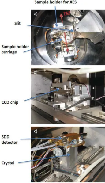
FIG. 1. Photograph of the von Hamos spectrometer of Fribourg as installed for
in-house XAFS measurements.
FIG. 2. Photograph of the internal part of the von Hamos vacuum chamber
show-ing (a) the sample holder and slit system (for XES measurements), (b) the CCD detector with the x-ray shutter, and (c) the crystal and silicon drift detector (SDD). The latter mounted on top of the crystal bending block serves to monitor the beam intensity during experiments at external facilities.
(seeFigs. 1–3), the dispersion axis is horizontal and the focusing direction vertical, the radius of curvature of the crystal is 25.4 cm, and the diffracted photons are measured with a position-sensitive CCD (charge-coupled device) detector. Depending on the photon energy, a back-illuminated (BI) CCD (1340× 400 pixels, with a pixel resolution of 20μm and a depletion depth of 15 μm) or a front-illuminated (FI) deep depleted CCD (1024× 256 pixels, with a pixel resolution of 27μm and a depletion depth of 50 μm) is used. Both CCD chips were manufactured by the English Electric Valve Com-pany (EEV)47for Roper Scientific48which provides complete CCD systems and related electronics and software. A detailed character-ization of the two CCD cameras is given in Ref.49. Thanks to the
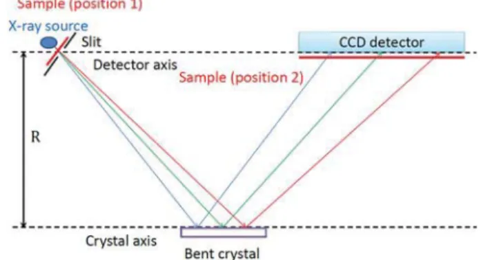
FIG. 3. Schematic drawing (top view) of the von Hamos setup for laboratory-based
XAFS measurements. The sample can be placed at either position (1) (in front of the slit) or position (2) (in front of the CCD detector). R stands for the radius of curvature of the crystal. The x-ray source corresponds to the electron beam spot on the x-ray tube anode.
energy resolution capability of the two CCDs (about 150 eV and 344 eV, respectively, at 5.9 keV), good event pixels are sorted online by setting on the ADC (analog-to-digital converter) of the CCD a charge window corresponding to the energy of the x-rays of interest. A narrow slit placed in front of the sample represents the effective source of radiation.
For a given position of the crystal and detector, photons within a certain energy range can be measured. The latter which depends mainly on the length (in the direction of dispersion) of the CCD varies between some tens to some hundreds of electronvolt. To cover a wider energy range, the crystal and detector are translated along axes that are parallel to the direction of dispersion, the detector twice as much as the crystal. Bragg angles between 24.4○and 63.2○can be achieved so that with the use of different crystals an energy range between 0.550 keV and 16.675 keV can be theoretically covered in the first order of diffraction. However, because of the weak effi-ciency of the CCD detectors below 1 keV and above 15 keV, the spectrometer is mostly used for x-ray energies between these two limits.
In XES measurements, since the sample should be located on the straight line joining the crystal center and the slit, upstream from the latter, the sample position must be changed whenever the Bragg angle is modified. This sample alignment is realized by translating the sample along the so-called TAF (target focus) axis (seeFig. 4 in Sec.II C) which is perpendicular to the direction of dispersion. The slit is mechanically coupled to the target carriage through a thin rod so that it remains automatically perpendicular to the direction defined by the sample and crystal centers for any TAF position. Dur-ing the measurements, the spectrometer chamber is evacuated down to about 10−6 hPa with a turbomolecular pump, and the sample, crystal, and detectors are moved, if needed, via remote-controlled stepping motors.
B. XAFS setup
For XAFS measurements, the spectrometer is operated in the so-called direct geometry.50In this geometry, the sample is replaced by the anode of a side-window x-ray tube that is mounted vertically
FIG. 4. Schematic drawing showing the lengths a, b, c, and d, and the angles φ,
γ, and ϑ (see text) for the case ϑ ≥ 41.3○.
on a rotatable flange located above the target chamber of the spec-trometer. A vacuum-tight feed through hole in the rotatable flange allows us to insert the x-ray tube nose into the target chamber. The x-ray tube is oriented so that the center of its beryllium window, the center of the slit, and the center of the crystal are all aligned along the direction determined by the Bragg angle corresponding to the cen-troid energy of the absorption edge to be measured (see Sec.II C). To reduce the scattering of the x-rays in the spectrometer chamber, a copper collimator with a 20 mm high× 5 mm wide rectangular aperture is mounted on the nose of the x-ray tube in front of the Be window.
XAFS measurements are performed in the transmission mode. The sample can be placed either in front of the slit or in front of the detector (seeFig. 3). When the sample is placed in front of the slit, the Bremsstrahlung from the x-ray tube passes first through the sample and then the transmitted radiation is analyzed by the crystal. When the sample is placed in front of the detector, the Bremsstrahlung is first monochromatized by the crystal and then the fraction of the diffracted radiation that is transmitted through the absorber is detected by the CCD. Note that in both cases, the transmitted intensity I(E) of the Bremsstrahlung x-rays belonging to the energy range selected by the crystal is measured in a straightfor-ward way by the CCD and there is no need to move any element of the spectrometer (scanless measurement).
When the absorber is placed in front of the CCD, the dimen-sions of the sample should be large enough to cover the CCD surface (2.68 × 0.80 cm2 and 2.76 × 0.69 cm2 for the BI and FI CCDs, respectively) and the thickness should be uniform to avoid a fake modulation of the transmitted intensity. In addition, because the Bragg angleϑ varies continuously along the dispersion axis of the CCD (seeFig. 3), the thickness h of the absorber can no longer be considered as constant and has to be replaced by h/sin(ϑ) in Eq.(5). Experimentally, it is also much easier to insert the absorber in front of the slit, i.e., between the x-ray tube and collimator, than in front of the CCD because the space between the x-ray shutter and front surface of the CCD chip is very narrow [seeFig. 2(b)]. For these rea-sons, all XAFS measurements presented below were performed with the absorber in front of the slit.
C. X-ray tube alignment
For the XAFS spectra presented in this work, 100 kV× 3 kW Coolidge-type side-window x-ray tubes from Malvern PANana-lytical with chromium and copper anodes were used. The thick-nesses of the tube windows made of beryllium were 0.5 mm and 0.3 mm, respectively. The water-cooled x-ray tubes were powered by a current- and voltage-stabilized x-ray generator, allowing to adjust digitally the voltage from 1 to 60 kV by 1 kV steps with an absolute precision of 2% and a stability of 0.01% and the current from 1 to 80 mA by 1 mA steps with an absolute precision of 1% and a stability of 0.01%.
The alignment of the x-ray tube that depends on the Bragg angle is realized by rotating the flange supporting the tube by an angleφ around a vertical axis passing through the flange center. The accuracy of the flange angular position is about 0.5○, but for a given angleφ, the reproducibility of the positioning for the measure-ments I0and I(E) is better (0.02○), thanks to a very simple optical system consisting of a laser pointer mounted on the flange and a reference mark on the laboratory wall behind the spectrometer. As the x-ray tube is not coaxial with the flange, an additional rotation of the tube around its axis by an angle γ is required to align the normal to the center of the x-ray tube window on the slit-crystal direction. The angleγ is indeed equal to zero only when the straight line joining the crystal and slit centers passes through the center of the flange. According to the schematic drawing presented inFig. 4, this condition is fulfilled for
ϑ = arctan[b
d]. (1)
As the distances b and d amount to 2.2 cm and 2.5 cm, respectively, ϑ = 41.3○. For Bragg anglesϑ ≠ 41.3○,γ reads as
γ = arcsin[a⋅ cos(ϑ)c ], (2)
where c = 4.5 cm and the length a is given by
a= d ⋅ tan(ϑ) − b. (3)
From the above two equations, one sees thatγ > 0 (anticlockwise rotation of the tube) forϑ > 41.3○andγ < 0 (clockwise rotation of the tube) forϑ < 41.3○. Finally, as shown inFig. 4, the angleφ can be written as
φ = 90○+ϑ + γ. (4)
Note that in the standard operation of the von Hamos spectrometer (XES measurements), the x-ray tube is positioned atφ = γ = 0. D. Methodology
The measurement of a XAFS spectrum is realized in the fol-lowing way: first, the crystal and detector are positioned according to the Bragg angle corresponding to the absorption edge of interest. The slit is set perpendicularly to the direction defined by the Bragg angle via the stepping motor of the TAF axis, and the x-ray tube is aligned according to the above-mentioned procedure [see Eqs.(2) and(4)]. The intensity I0(E) of the Bremsstrahlung corresponding to the selected energy region is measured, and then, the measurement is repeated using exactly the same positions for the crystal, detector,
and slit, as well as the same orientation, high voltage, and current of the x-ray tube, but this time the sample to be analyzed is inserted in front of the slit or in front of the CCD detector. This second measurement provides the intensity I(E). The attenuation coefficient μ(E) for the photon energy E is then deduced from the Beer-Lambert law using the following equation:
μ(E) =ln(
I0(E)
I(E))
ρh , (5)
whereρ is the density of the sample and h its thickness.
The thicknesses of the samples were determined from their measured areas S and masses m and their tabulated densitiesρ as
h= m
ρA. (6)
Note that the sample thickness should be chosen so that the differ-ence between the intensities I0and I of the incident and transmitted beams is large, keeping I, however, at a reasonably high enough value. A too thick absorber leads indeed to an attenuation of the x-ray absorption near edge structure (XANES) oscillations and to
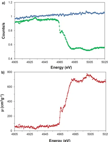
FIG. 5. (a) Measured incident (blue circles) and transmitted (green circles) photon
intensities around the K-edge of Ti. (b) Attenuation coefficient μ(E) deduced from (a). The red line is a smoothed curve to guide the eye. The Ti foil thickness was 2.07(5)μm, and the Cr anode x-ray tube was operated at 10 kV × 10 mA. The measurement was performed using a Si(220) crystal, and the acquisition times were 8000 s and 30 000 s for the measurements of I0and I(E), respectively.
a reduction in the white line intensity, resulting in an apparent shift of the absorption edge energy with the sample thickness.51,52As a rule of thumb, it is generally recommended to choose the absorber thickness h so that 2< μρh < 4. To preserve the white line shape and intensity, an even smaller sample thickness given byμmaxρh
≤ 1, where μmaxrepresents the maximum value of the attenuation
coefficient in the scanned energy region, is suggested in Ref.53. For illustration, the intensities I0(E) and I(E) and the result-ing attenuation coefficientμ(E) are depicted for the K-edge of Ti in Fig. 5. The first peak observed in the absorption spectrum at 4965 eV corresponds to the white line. The latter is due to the large unoc-cupancy of nd states in transition metals.54The small peak around 4930 eV in the I(E) spectrum and the corresponding small hole in the absorption spectrum originate from the Kβ1,3 x-ray line of Ti (4931.81 eV). This possibility of having absorption edges and emission lines on the same energy scale represents an interesting feature55of the present system.
III. COMPARISON WITH SYNCHROTRON RADIATION MEASUREMENTS
At synchrotron radiation facilities, XAFS measurements are usually performed by scanning the energy of the beam around the absorption edge. In other words, the XAFS spectra are measured step by step, but the intensities I0(E) and I(E) are determined simulta-neously and the acquisition time per energy step typically is in the order of 0.1–1 s depending on the experimental method, SR beam-line conditions, and sample elemental concentration. As a conse-quence, a 200 eV wide XAFS spectrum can be measured in less than 15 min, whereas 2–5 h are needed to measure the same spectrum with a laboratory-based XAFS setup as the one presented in this work. Furthermore, the quick-scanning XAFS acquisition technique and the energy-dispersive approaches allow reaching even subsec-ond to -minute time resolution for a XAFS spectrum data collec-tion.56Thus, XAFS setups based on conventional x-ray sources can-not compete in terms of measuring times with synchrotron radiation sources, but in most cases, this is not a big disadvantage because the time constraints are not as severe at home as at external big facilities. It should be also noted that in SR-based XAFS measure-ments, the main interest resides in the determination of the edge energies and XANES oscillations and not in the values of the atten-uation coefficients μ(E), because in the fluorescence and electron yield XAFS techniques that are most commonly used at SR facili-ties, the coefficientsμ(E) cannot be determined in a straightforward way.
Despite the above-mentioned differences, XAFS spectra obtained from laboratory-based measurements can be compared with those measured at SR facilities to validate the methodology and the setup used in-house. Such comparisons were done in the present work for the Cu K and Ta L3XAFS spectra. The results are presented inFigs. 6and7, respectively.
The SR-based measurement of the Cu K-edge spectrum was performed in the fluorescence mode at the beamline SuperXAS of the Swiss Light Source (SLS). The in-house experiment was per-formed with a 3-μm-thick foil, a Cr x-ray tube operated at 15 kV × 15 mA, and a SiO2(2¯23) crystal. Collecting times of 5000 s and 30 000 s were used for the measurements of I0 and I(E), respec-tively. The SLS and Fribourg spectra were normalized to overlap
FIG. 6. Shape comparison between the Cu K-edge absorption spectrum measured
at SLS in the fluorescence mode (black solid line) and the corresponding spectrum measured in Fribourg with the laboratory-based setup (red points). The relative uncertainties of the points measured in Fribourg amount to about 10% (below the edge) and 3% (above the edge), respectively. The SLS plot was taken from Ref.41.
as well as possible below and above the edge. As shown, the over-all shape of the two spectra is very similar, although the spectrum measured at home is more noisy due to the much weaker photon flux of the conventional x-ray source as compared with the one of the SR beam. On the other hand, the midedge shoulder (at about 8982 eV) of the spectrum measured in Fribourg is slightly shifted toward higher energy and a little bit broader. The difference in the midedge shoulder width is due to the better energy resolution of the SLS measurement, whereas the energy difference of about 2 eV was assumed to originate from the bigger scatter of the in-house data.
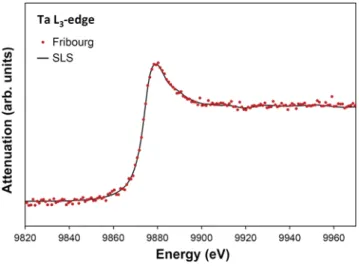
The second comparison concerns the L3XAFS spectrum of a 5-μm-thick metallic foil of Ta. The SR-based measurement was again performed at the SuperXAS beamline of SLS, but this time
FIG. 7. Same asFig. 6but for the Ta L3XAFS spectrum. In this case, the SLS data
(taken from Ref.39) were collected in the transmission mode.
in the transmission mode. The measurement of Fribourg was per-formed with a Ge(440) crystal and a Cr anode x-ray tube operated at 25 kV× 40 mA. Collecting times of 4000 s (I0) and 17 000 s I(E) were employed. As can be seen inFig. 7, the SLS and Fribourg Ta L3XAFS spectra are in excellent agreement, except at about 9956 eV where a small excess of absorption is observed in the spectrum mea-sured at home. The difference, however, is hardly significant within the uncertainty of the experimental data.
IV. EDGE ENERGIES AND ATTENUATION COEFFICIENTS
To check the reliability and accuracy of the in-house XAFS setup, measurements of the absorption spectra around the K-edges of Ti, Fe, Cu, and Ge, and around the L3-edges of Mo, Ag, Hf, Ta, and Pt were performed. For Mo and Ag, the XAS spectra around the L2- and L1-edges were also measured. All measurements were performed with the same slit width of 0.2 mm but with different crystals and different high voltages of the x-ray tube. From the mea-surements, the edge energies and the attenuation coefficients below and above the edges were determined.
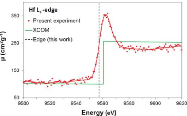
For illustration, the L3-edge absorption spectrum of Hf is pre-sented in Fig. 8and compared with data from the NIST XCOM database.57 As the latter do not take into account the processes leading to the XANES and EXAFS structures, plots of the XCOM data over narrow energy ranges correspond to quasistraight lines with slightly negative slopes and a sudden jump of the attenuation coefficient to bigger values at the edge energy.
A. Edge energies
The location of an absorption edge is not unambiguously defined58and has been variously associated in the literature with (i) the first inflection point of the absorption spectrum, (ii) the energy
FIG. 8. L3-edge XAFS spectrum of Hf. The measurement was performed with a
2.84(7)-μm-thick sample, a Si(333) crystal, and a copper anode x-ray tube oper-ated at 15 kV× 20 mA. The I0and I(E) spectra were collected in 13 000 s and
30 000 s, respectively. The spectrum was calibrated in energy from measurements of the Kα1x-ray lines of Zn and Ge, using the values reported in Ref.58for the
energies of these transitions. The position of the L3-edge is indicated by the vertical
dashed line. The green solid line corresponds to the energy-dependent absorp-tion coefficientμ(E) from the XCOM database (see text). The red solid line (data smoothing) serves only to guide the eye.
needed to produce a single core vacancy with the photoelectron “at rest at infinity,” and (iii) the energy needed to promote a core elec-tron to the lowest unoccupied state. Note that in the alternative (ii), the absorption edge energies can be determined by combining the electron binding energies of outer shells which can be measured accurately by means of photoelectron spectroscopy with the ener-gies of emission lines involving transition electrons which originate from these outer shells.
The measured XAFS spectra were calibrated in energy by mea-suring reference K x-ray lines with energies smaller and bigger than the edge energies of interest. The energies of the reference lines were taken from Ref.58. The method used for the energy calibration of the von Hamos spectrometer is not presented here because it was already described in detail elsewhere (see, e.g., Refs.45and59). In this work, the edge energies were associated with the first inflec-tion points of the absorpinflec-tion spectra. The derivative of the funcinflec-tion μ(E) was computed numerically and then fitted with a Gaussian function. For illustration, the L3absorption spectrum of Mo and the first derivative of the latter are presented inFig. 9. The max-imum value of the derivative which coincides with the inflection point was determined from the energy corresponding to the cen-troid of the fitted Gaussian function since for symmetric functions the energy corresponding to the maximum value of the function coincides with the centroid of the latter. It was found that the deter-mination of the inflection point was not really sensitive to the choice of the function employed to fit the derivative dμ(E)/dE. Actually, no significant differences could be evinced between the edge ener-gies obtained from the fits of the derivatives performed with Gauss, Lorentz, or Voigt functions. For example, for the K-edge of Cu, val-ues of 8980.53± 0.44 eV, 8980.42 ± 0.42 eV, and 8980.58 ± 0.39 eV were found by fitting the derivative of the XAFS spectrum with a Gaussian, Lorentzian, and Voigtian function, respectively. As the choice of the fit function was found to be not critical, Gaussian functions were employed for all edges investigated in the present work.
FIG. 9. Mo L3-edge spectrum (red circles) and its first derivative (blue line). The
edge energy represented by the vertical dashed line was determined from the centroid of the Gaussian used to fit the derivative in the edge region. The mea-surement was performed with a 1.24(3)-μm-thick metallic foil, a Si(111) crystal, and a Cu anode x-ray tube operated at 4 kV× 9 mA. Due to the low value of the employed high voltage, long acquisition times were needed [40 000 s for I0and
60 000 s for I(E)].
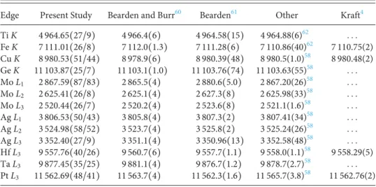
TABLE I. Comparison between the edge energies determined with the present XAFS setup and other existing experimental values. All energies are given in eV. The notation 4964.65(27/9) means 4964.65± 0.27 with an included fit error of 0.09.
Edge Present Study Bearden and Burr60 Bearden61 Other Kraft4
Ti K 4 964.65(27/9) 4 966.4(6) 4 964.58(15) 4 964.88(6)62 . . . Fe K 7 111.01(26/8) 7 112.0(1.3) 7 111.28(6) 7 110.86(40)62 7 110.75(2) Cu K 8 980.53(51/44) 8 978.9(6) 8 980.39(48) 8 980.5(1.0)58 8 980.48(2) Ge K 11 103.87(25/7) 11 103.1(1.0) 11 103.76(74) 11 103.63(55)58 . . . Mo L1 2 867.59(87/83) 2 865.5(4) 2 880.6(5.0) 2 867.20(26)58 . . . Mo L2 2 625.41(26/8) 2 625.1(4) 2 627.3(8) 2 625.98(33)58 . . . Mo L3 2 520.44(26/7) 2 520.2(4) 2 523.6(8) 2 521.1(1.6)58 . . . Ag L1 3 806.53(50/43) 3 805.8(4) 3 807.3(2) 3 807.41(34)58 . . . Ag L2 3 524.98(58/52) 3 523.7(4) 3 525.8(2) 3 525.24(26)58 . . . Ag L3 3 352.40(27/9) 3 351.1(4) 3 350.96(13) 3 352.58(48)58 . . . Hf L3 9 557.76(40/26) 9 560.7(6) 9 557.7(1.1) 9 558.0(1.1)58 9 558.29(5) Ta L3 9 877.45(35/25) 9 881.1(4) 9 876.7(1.2) 9 878.7(2.7)58 . . . Pt L3 11 562.69(48/41) 11 563.7(4) 11 562.3(1.6) 11 565.7(3.8)58 11 562.76(2)
The uncertainties on the edge energies quoted inTable I corre-spond to the uncertainties given by the fits for the Gaussian centroids combined with the uncertainties originating from the energy cal-ibration measurements. The latter include the uncertainties of the reference line energies, the uncertainties originating from the fits of these reference lines, as well as the uncertainties related to the CCD positions. The latter can be determined with a precision of±1 μm, thanks to a dedicated optical system.
The edge energies obtained in this work are presented inTable I where they are compared with experimental values reported by Bear-den and Burr,60 Bearden,61 Sevier,62 Deslattes et al.,58 and Kraft et al.4The values reported by Bearden and Burr were obtained from photoelectron spectroscopy measurements, those from Sevier and Deslattes were determined by adding to the energies of K and L x-ray transitions from outer levels the known energies of the latter, while the results obtained by Kraft were derived from synchrotron radia-tion measurements and the first inflecradia-tion point method. Regarding the edge energies reported by Bearden, no indication is provided in Ref.61about the employed method. The edge energies quoted in the XCOM database57(see, e.g.,Fig. 7) are those of Bearden and Burr.60 FromTable I, one sees that the edge energies reported by Bear-den and Burr60are all inconsistent with ours, except for the L2- and L3-edges of Mo. The discrepancy cannot be explained by the differ-ent definitions of the edge energy used in our work (inflection point of lowest energy) and the one of Bearden and Burr (binding energy of the 1s electron), because some values from Ref.60are bigger than ours, some other ones smaller.
The comparison with Bearden’s values61 is more satisfactory since the latter are in agreement with ours for the K-edges and for the L3-edges of Hf, Ta, and Pt, whereas for the L1–3-edges of Mo and Ag, discrepancies are observed. Actually, except for the L3-edge energy of Ag which is slightly smaller than ours, the other L-edge energies of these two elements are significantly bigger than our values. In the case of the L1-edge of Mo, the energy quoted by Bearden overes-timates even our result by about 13 eV. We guess, however, that some problems were encountered by Bearden in this measurement
because the error of±5 eV reported for this edge is much bigger than the uncertainties quoted for the other edges.
A satisfactory agreement is observed in the comparison of present values with those reported by Sevier62and Deslattes et al.58 As mentioned before, the latter were obtained from x-ray transition energies combined with the known binding energies of the outer levels involved in these transitions. Actually, the K-edge energies of Ti and Fe reported by Sevier are very close to our values, while the data from Deslattes are also in good agreement with the results obtained in the present work, except for the L2-edge of Mo (devi-ation of 1.3σ, where σ stands for the combined error of the two results) and L1-edge of Ag (1.4σ). The L3-edge energy of Pt reported by Deslattes is 3 eV bigger than our value but nevertheless consistent with it because in this case the error quoted by Deslattes is quite big (3.8 eV).
Finally, the present edge energies are consistent with the data reported by Kraft et al.4 for the K-edges of Fe and Cu and the L3 -edge of Pt, whereas a deviation of about 1.3σ is observed for the L3 -edge of Hf. The values of Kraft represent probably the most precise and reliable reference data for checking the accuracy of the present values, but unfortunately, Fe, Cu, Hf, and Pt are the single elements common to both experiments.
B. Attenuation coefficients
The attenuation coefficientsμ(E) were determined from the measured intensities of the incoming (I0) and transmitted (I) photon beams using Eq.(5). The observed variation of the incoming beam intensity I0with the energy [seeFig. 5(a)] reflects the energy dis-tribution of the Bremsstrahlung emission of the x-ray tube as well as the inhomogeneous intensity of the electron beam spot on the anode of the tube. However, as the experimental setup is exactly the same in the measurements of I0(E) and I(E), the same variations are observed in the spectrum I(E) and the latter do not affect, thus, the determination of the absorption coefficient.
In the XCOM tables,57for each edge energy, two values are given which correspond to the attenuation coefficients just before
and after the jump, i.e., toμb=μ(E→<Eedge) and μa=μ(E→>Eedge).
Thus, for the comparison of the present attenuation coefficients with the data from the XCOM database,57linear functions were fitted to the XAFS data below and above the edges and the valuesμbandμa
reported inTable IIwere then obtained by calculating the values of the two linear functions for E = Eedge.
Neglecting the uncertainty on the density of the sample, the uncertainty on the absorption coefficientμ reads as
Δμ =√σ2
fit+σh2+σ2tube, (7)
whereσfitrepresents the uncertainty from the linear fitting of the
data below and above the edge,σhrepresents the uncertainty
origi-nating from the uncertainty on the sample thickness, andσtube
rep-resents the uncertainty accounting for the intensity variation of the x-ray tube between the I0(E) and I(E) measurements. The uncer-taintyσhis simply given by
σh= ∣∂μ
∂hΔh∣ =Δhh μ, (8)
whereasσtubecan be expressed as a function of the parameterξ
rep-resenting the variation of the x-ray tube intensity between the I0(E) and I(E) measurements,
I(E) = ξI0(E)e−μ(E)ρh, (9)
which leads to σtube= 1 ρh Δξ ξ . (10)
The relative uncertaintyΔξ/ξ was assumed to be 2%.
The attenuation coefficients determined in the present work for photon energies just below and above the edges are presented inTable II, where they are compared with values from the XCOM database57and from the tables of Storm and Israel63and Henke.64 In the latter reference, the reported values are only given for
energies corresponding to strong K and L x-ray lines of selected ele-ments. For this reason, the coefficientsμb(Eedge) andμa(Eedge) listed
inTable IIwere determined from double logarithmic interpolations of the values quoted in Ref.64for transition energies below and above the edges of interest. However, as only one or even no value is reported between the L1- and L2-edges and between the L2- and L3-edges, in the case of the L-shell, only the coefficientsμb(EL1−edge) andμa(EL3−edge) could be derived.
In the tables of Storm and Israel, it is stated that the relative uncertainties of the attenuation coefficients are in the order of 10%, whereas no indication could be found about the uncertainties affect-ing the values listed in the XCOM57and Henke64tables. However, as the values from the three databases are based on similar approaches, the same relative uncertainty of 10% was assumed for the values quoted in these tables. With this assumption, one can see from the inspection ofTable II that all attenuation coefficients determined in the present work are in agreement within the combined uncer-tainties with the values reported in the three databases, except for the coefficients μa of Fe and Ge and the coefficientμb of the Ag
L3-edge which are bigger than the theoretical predictions and dif-fer from the average values of the latter by about 1.4σ, 1.5 σ, and 1.1 σ, respectively.
Accurate experimental values for the mass attenuation coeffi-cientsμ(E) are scarce in the literature. However, some data from the Laboratoire National Henri Becquerel (LNHB, Paris) were found for the K-edges of Ti,65 Cu,66 and Ge,67 and the L3-edges of Hf and Pt.67These recent experimental XAFS data that were obtained partly at the metrology beamline of the synchrotron radiation facil-ity SOLEIL68 and partly with the tunable monochromatic x-ray source SOLEX69 are reliable and precise. To obtain the attenua-tion coefficients μb(Eedge) and μa(Eedge) from the values tabulated
in Refs.65–67, the same method as the one used for our own data was employed, namely linear spline interpolations below and above the edges. For Hf, the strong white line was excluded from the interpolation domain. The obtained values are presented inTable II,
TABLE II. Comparison between the attenuation coefficients μb(below the edge) andμa(above the edge) obtained with the present XAFS setup and values from the existing databases. For the K-edges of Cu and Ge and the L3-edges of Hf and Pt, the comparison was extended to the recent and precise experimental values determined at the “Laboratoire National Henri Becquerel” (LNHB). All values are given in cm2/g.
Present Study XCOM57 Storm and Israel63 Henke64 LNHB
Edge μb μa μb μa μb μa μb μa μb μa Ti K 74(11) 716(22) 84 684 84 708 83 718 82.2(2)65 737.2(1.1)65 Fe K 55(7) 352(11) 53 408 53 414 51 412 . . . . . . Cu K 40(4) 309(9) 38 278 38 285 37 289 37.5(1)66 305.6(1.3)66 Ge K 30(12) 237(12) 28 198 28 202 27 208 27.8(2)67 207.6(7)67 Mo L1 1943(48) 2259(56) 1961 2243 1952 2235 . . . 2245 . . . . . . Mo L2 1652(41) 2518(71) 1750 2433 1758 2410 . . . . . . . . . . . . Mo L3 597(17) 1924(53) 542 1979 539 1940 542 . . . . . . . . . Ag L1 1317(35) 1471(39) 1282 1468 1267 1457 . . . 1465 . . . . . . Ag L2 1132(30) 1507(40) 1126 1547 1122 1535 . . . . . . . . . . . . Ag L3 432(14) 1205(33) 389 1274 386 1267 385 . . . . . . . . . Hf L3 101(4) 252(7) 100 256 99 262 102 . . . 97.8(2)67 248.4(5)67 Ta L3 104(4) 230(7) 96 244 95 250 93 . . . . . . . . . Pt L3 78(3) 196(6) 78 195 77 197 76 . . . 75.1(1)67 186.2(3)67
http://doc.rero.ch
where they are compared with the present results. As can be seen, a quite satisfactory agreement is observed, except for the coeffi-cientsμaof the K-edge of Ge and the L3-edge of Pt for which our values are bigger than those of LNHB by about 2.4σ and 1.6 σ, respectively.
V. COMPARISON BETWEENK -EDGE XAFS SPECTRA
OF METALLIC IRON AND IRON OXIDES
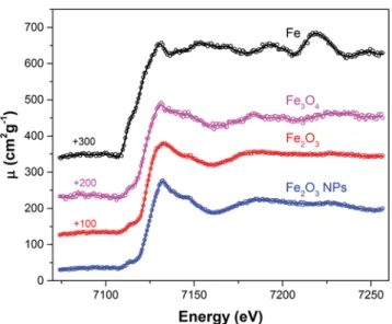
Samples of metallic Fe (Fe0) and Fe2O3 (Fe3+) and Fe3O4 (Fe2+,3+) oxides were measured. To probe the sensitivity of the XAFS spectra to the size of the particles in the case of powder samples, two Fe2O3powders were measured: the first one with a particle size of ≤5 μm and the second one with a particle size of 5–25 nm. The grain size of the Fe3O4powder was also≤5 μm. The sample thicknesses were 1.62 mg/cm2, 2.80 mg/cm2, 1.80 mg/cm2, and 2.95 mg/cm2for the metallic Fe foil, Fe2O3, Fe3O4powders, and Fe2O3 nanopow-der, respectively. The measurements were performed with a Cu x-ray tube operated at 40 kV× 30 mA and a SiO2(2¯23) crystal. The acqui-sition time was 10 000 s for each spectrum. Because residuals of the Kα1,2characteristic x-ray lines of Cu from the tube were observed in the spectrum during test measurements, a 20-μm-thick foil of Co was installed in front of the collimator as a filter, resulting in an attenuation by a factor 2.8 of the good signal and by a factor of about 300 of the parasitic Kα1,2lines of Cu. The energy calibration of the spectra was performed by measuring the Kα1 lines of Co and Ni, using the transition energies reported in Ref.58as references.
The four XAFS spectra are depicted inFig. 10. As can be seen, obvious differences are observed in the XANES oscillations between Fe metal and Fe oxides as well as between the micropowder and nanopowder samples of Fe2O3. For each absorber, the edge energy was determined with the first inflection point method. Values of
FIG. 10. Comparison between the K-edge XAFS spectra of metallic Fe, Fe2O3,
and Fe3O4oxides. For Fe2O3, two samples with grain sizes of≤5 μm and 5–25
nm (NPs) were measured. For clarity, offsets in the vertical scale of +100, +200, and +300 cm2/g were used for the XAFS spectra of Fe
2O3, Fe3O4, and Fe metal,
respectively.
7110.82(2) eV, 7111.78(6) eV, 7111.89(9) eV, and 7111.97(6) eV were found for Fe, Fe3O4, Fe2O3, and Fe2O3NPs, respectively. Note that for metallic Fe, the edge energy is consistent within the com-bined uncertainties, with the value of 7111.01(26) eV (seeTable I) found in another measurement performed with the Cr x-ray tube and very close to the value of 7110.75 eV obtained by Kraft4 with SR. Regarding the difference of 0.08 eV between the edge energies of the Fe2O3micro- and nanopowder samples, no definitive conclusion can be drawn because this difference is smaller than the combined uncertainty of 0.11 eV. Furthermore, assuming that the energy shift of the oxide edges varies linearly with the degree of oxidation, one finds that the average oxidation state of Fe3O4should be 2.69(17), in good agreement with the expected value of 2.67 corresponding to the known valence ratio of 1/2, i.e., 1/3 Fe2+and 2/3 Fe3+, of the Fe2O3 oxide.
VI. SUMMARY AND CONCLUDING REMARKS
A laboratory-based setup for in-house XAFS measurements was developed and commissioned. The setup is based on the von Hamos bent crystal spectrometer of Fribourg, and the source of radi-ation is an x-ray tube. The new setup was validated by measuring the XAS spectra around the K-edges and L-edges of several solid samples. The shapes of the K-edge of Cu and L3-edge of Ta were compared with those measured with synchrotron radiation at the SLS. The spectra were found to overlap very well in both cases. The sensitivity to chemical effects of the XAFS spectra measured with the in-house setup was demonstrated for metallic Fe and Fe oxides. Fur-thermore, the edge energies and attenuation coefficients below and above the K-edges of Ti, Fe, Cu, and Ge, L1–3-edges of Mo and Ag, and L3-edges of Hf, Ta, and Pt were extracted from the measure-ments and compared with the data from the existing theoretical and experimental databases.
The present edge energies were determined from the inflec-tion points of lowest energy. The so-determined edge energies were found to be in good agreement with the recent and reliable values obtained with synchrotron radiation4and with values derived from x-ray transition energies combined with the energies of the outer levels involved in these transitions.58 In contrast to that, most of the edge energies reported by Bearden61and to a smaller extent by Bearden and Burr60were found to be inconsistent with our values.
The attenuation coefficients just below and just above the edges were determined by calculating the values at the edge energies of the linear functions obtained from spline interpolations of the XAFS data points measured below and above the edges. The results were compared with values from three different databases, namely the NIST XCOM,57Storm and Israel,63and Henke64databases, and to the recent experimental data from the LNHB.65–67In both cases, a quite good agreement was observed, except for Ge and Pt for which the present attenuation coefficients above the edge were found to slightly overestimate the literature values.
A clear advantage of the in-house setup presented in this work is its simplicity and better availability as compared with the SR-based equipment. In counterpart, the data taken with the laboratory-based setup are more noisy due to the significantly lower intensity of the employed x-ray source. For the same reason, the data col-lection times are longer than at SR facilities by about one order of magnitude for standard XAFS measurements. Actually, to avoid a
contamination of the XAFS spectra by higher energy photons, most of the present measurements were performed at low values of the x-ray tube voltage and current, i.e., with detected photon intensi-ties I0(E) in the order of several photons/s. However, thanks to the energy resolution capability of the CCD, higher energy photons can be suppressed very efficiently by applying narrow energy windows to the CCD so that probably most of the measurements could have been performed at higher x-ray tube voltages (e.g., 60 kV) and cur-rents and thus with about 10–20 times higher incoming photon intensities. It should be noted, however, that the CCD detector is count rate limited to about 20 photons/s over the 400 (BI CCD) or 256 (FI CCD) pixels in the nondispersive direction in order to avoid multiple hit events. As depicted inFig. 5for the K-edge of Ti mea-sured at 10 kV and 10 mA, I0(E) is about 1 photon/s. The 40 kV × 30 mA x-ray tube operating conditions for the Fe XAFS spectra (Fig. 10) yield I0(E) count rates of 5.5 photons/s. In the case of the Ta XAFS shown inFig. 7, for I0(E), count rates of 20 photons/s at an operating voltage of 25 kV and current of 40 mA for a Cr x-ray tube were achieved. The present I0(E) count rate of 20 photons/s is thus comparable with the one of about 30 photons/s reported in Ref.30 for the NiO K-edge measurement at 10 kV× 40 mA.
A further weak point of the in-house setup resides in the fact that the spectra I0(E) and I(E) are not measured simultaneously but sequentially. This drawback could be eliminated, however, by moni-toring the x-ray tube intensity with a SDD detector placed above the crystal, but then the sample should be placed in front of the CCD and not in front of the slit. An elegant alternative solution would consist to place again the sample in front of the CCD but to cover only the top half part of the latter (i.e., rows 201–400 for the BI CCD) with the sample and to leave the bottom part (rows 1–200) uncov-ered. By projecting then separately the top and bottom CCD rows onto the dispersion axis, simultaneous I(E) and I0(E) spectra would be obtained. In the latter two cases, however, the sample should be at least as long as the CCD, be free of pinholes, and have a highly homogeneous thickness.
In conclusion, it has been proven that XAFS measurements are feasible by means of the presented in-house setup and that the obtained results (XAFS spectrum shapes, edge energies, and atten-uation coefficients) are reliable. Although laboratory-based XAFS setups cannot compete with the SR-based ones in terms of pho-ton beam intensities and the duration of the measurements, the two techniques can be considered as complementary and both useful for academic research and industrial applications.
ACKNOWLEDGMENTS
The financial support of the Swiss National Science Foundation is acknowledged (Grant No. 200020-146739).
REFERENCES
1L. A. Grunes,Phys. Rev. B27, 2111 (1983).
2K. W. Nam, W. S. Yoon, and K. B. Kim,Electrochim. Acta47, 3201 (2002). 3T. Matsushita and R. P. Phizackerley,Jpn. J. Appl. Phys., Part 120, 2223 (1981). 4S. Kraft, J. Stümpel, P. Becker, and U. Kuetgens,Rev. Sci. Instrum.67, 681 (1996). 5T. J. Regan, C. Stamm, F. Nolting, J. Lüning, J. Stöhr, and R. L. White,Phys. Rev. B64, 214422 (2001).
6I. J. Pickering, R. C. Prince, T. Divers, and G. N. George,FEBS Lett.441, 11
(1998).
7
M. E. Fleet, C. T. Herzberg, G. S. Henderson, E. D. Crozier, M. D. Osborne, and C. M. Scarfe,Geochim. Cosmochim. Acta48, 1455 (1984).
8L. M. Miller, Q. Wang, T. P. Pelivala, R. J. Smith, A. Lanzirotti, and J. Miklossy, J. Struct. Biol.155, 30 (2006).
9
D. E. Salt, R. C. Prince, A. J. M. Baker, I. Raskin, and I. J. Pickering,Environ. Sci. Technol.33, 713 (1999).
10M. G. Dowsett and A. Adriaens,Anal. Chem.78, 3360 (2006).
11S. Reguer, P. Dillmann, F. Mirambet, J. Susini, and P. Lagarde,Appl. Phys. A83,
189 (2006).
12
D. E. Sayers, E. A. Stern, and F. W. Lytle, Phys. Rev. Lett. 27, 1204
(1971).
13F. W. Lytle, D. E. Sayers, and E. A. Stern,Phys. Rev. B11, 4825 (1975). 14
E. A. Stern, D. E. Sayers, and P. W. Lytle,Phys. Rev. B11, 4836 (1975). 15E. A. Stern, Laboratory EXAFS Facilities (American Institute of Physics, New
York, 1980).
16K. Nishihagi, A. Kawabata, and K. Taniguchi,Jpn. J. Appl. Phys., Part 132, 258
(1993).
17
Y. Inada, S. Funahashi, and H. Ohtaki,Rev. Sci. Instrum.65, 18 (1994). 18P. Lecante, J. Jaud, A. Mosset, J. Galy, and A. Burian,Rev. Sci. Instrum.65, 845
(1994).
19J. Hoszowska and J.-Cl. Dousse,J. Phys. B: At., Mol. Opt. Phys.29, 1641
(1996).
20Y. Inada and S. Funahashi,Z. Naturforsch.52, 711 (1997). 21K. Sakurai and X. M. Guo,Spectrochim. Acta, Part B54, 99 (1999). 22
T. Taguchi, Q. F. Xiao, and J. Harada,J. Synchrotron Radiat.6, 170 (1999). 23T. Taguchi, J. Harada, A. Kiku, K. Tohji, and K. Shinoda,J. Synchrotron Radiat.
8, 363 (2001).
24T. Taguchi, K. Shinoda, and K. Tohji,Phys. Scr.T115, 1017 (2005).
25Y. N. Yuryev, H.-J. Lee, H.-M. Park, Y.-K. Cho, and M.-K. Lee,Rev. Sci. Instrum.
78, 025108 (2007).
26M. Szlachetko, M. Berset, J.-Cl. Dousse, J. Hoszowska, and J. Szlachetko,Rev. Sci. Instrum.84, 093104 (2013).
27G. T. Seidler, D. R. Mortensen, A. J. Remesnik, J. I. Pacold, N. A. Ball, N. Barry,
M. Styczinski, and O. R. Hoidn,Rev. Sci. Instrum.85, 113906 (2014).
28
C. Schlesiger, L. Anklamm, H. Stiel, W. Malzer, and B. Kanngiesser,J. Anal. At. Spectrom.30, 1080 (2015).
29
I. Mantouvalou, K. Witte, W. Martyanov, A. Jonas, D. Grötzsch, C. Streeck, H. Löchel, I. Rudolph, A. Erko, H. Stiel, and B. Kanngießer,Appl. Phys. Lett.108,
201106 (2016).
30Z. Németh, J. Szlachetko, E. G. Bajnóczi, and G. Vankó,Rev. Sci. Instrum.87,
103105 (2016).
31J. G. Moya-Cancino, A.-P. Honkanen, A. M. J. van der Herden, H. Schaink,
L. Folkertsma, M. Ghiasi, A. Longo, F. M. F. de Groot, F. Meirer, S. Huotari, and B. M. Weckhuysen,ChemCatChem11, 1039 (2019).
32E. P. Jahrman, W. M. Holden, A. S. Ditter, D. R. Mortensen, G. T. Seidler, T.
T. Fister, S. A. Kosimor, L. F. J. Piper, J. Rana, N. C. Hyatt, and M. C. Stennett,
Rev. Sci. Instrum.90, 024106 (2019).
33
G. T. Seidler, D. R. Mortensen, A. S. Ditter, N. A. Ball, and A. J. Remesnik,J. Phys.: Conf. Ser.712, 012015 (2016).
34R. Bès, T. Ahopelto, A.-P. Honkanen, S. Huotari, G. Leinders, J. Pakarinen, and
K. Kvashina,J. Nucl. Mater.507, 50 (2018).
35A.-P. Honkanen, S. Hollikkala, T. Ahopelto, A.-J. Kallio, M. Blomberg, and
S. Huotari,Rev. Sci. Instrum.90, 035002 (2019).
36W. Blachucki, J. Czapla-Masztafiak, J. Sá, and J. Szlachetko,J. Anal. At. Spec-trom.34, 1409 (2019).
37J. Jaklevic, J. A. Kirby, M. P. Klein, A. S. Robertson, G. S. Brown, and P.
Eisen-berger,Solid State Commun.23, 679 (1977).
38W. Gudat and C. Kunz,Phys. Rev. Lett.29, 169 (1972).
39W. Blachucki, J. Szalchetko, J. Hoszowska, J.-Cl. Dousse, Y. Kayser, M.
Nachte-gaal, and J. Sá,Phys. Rev. Lett.112, 173003 (2014).
40J. Szlachetko, M. Nachtegaal, J. Sá, J.-Cl. Dousse, J. Hoszowska, E. Kleymenov,
M. Janousch, O. V. Safonova, C. König, and J. A. van Bokhoven,Chem. Commun.
48, 10898 (2012).
41
J. Szlachetko, C. J. Milne, J. Hoszowska, J.-Cl. Dousse, W. Blachucki, J. Sá, Y. Kayser, M. Messerschmidt, R. Abela, S. Boutet, C. David, G. Williams, M. Pajek, B. D. Patterson, G. Smolentsev, J. A. van Bokhoven, and M. Nachtegaal,Struct.
Dyn.1, 021101 (2014).
42J. Szlachetko, J. Sá, M. Nachtegaal, U. Hartfelder, J.-Cl. Dousse, J. Hoszowska,
D. L. Abreu Fernandes, H. Shi, and C. Stampfl,J. Phys. Chem. Lett.5, 80 (2014). 43W. Blachucki, J. Hoszowska, J.-Cl. Dousse, Y. Kayser, R. Stachura, K. Tyrala,
K. Wojtaszek, J. Sá, and J. Szlachetko,Spectrochim. Acta, Part B136, 23 (2017). 44W. Blachucki, J. Szlachetko, Y. Kayser, J.-Cl. Dousse, J. Hoszowska, F. Zeeshan,
and J. Sá,Nucl. Instrum. Methods Phys. Res., Sect. B411, 63 (2017).
45J. Hoszowska, J.-Cl. Dousse, J. Kern, and C. Rhême,Nucl. Instrum. Methods Phys. Res., Sect. A376, 129 (1996).
46L. von Hamos,Ann. Phys.409, 716 (1933).
47Seehttps://www.teledyne-e2v.com/ for details about English Electric Valve
Company (now Teledyne e2v).
48Seewww.roperscientific.comfor details about this Roper Scientific.
49J. Szlachetko, J.-Cl. Dousse, J. Hoszowska, M. Berset, W. Cao, M. Szlachetko,
and M. Kavˇciˇc,Rev. Sci. Instrum.78, 093102 (2007).
50F. Zeeshan, J.-Cl. Dousse, and J. Hoszowska, J. Electron Spectrosc. Relat. Phenom.233, 11 (2019).
51L. G. Parratt, C. F. Hempstead, and E. L. Jossem,Phys. Rev.105, 1228 (1957). 52M. Bianchini and P. Glatzel,J. Synchrotron Radiat.19, 911 (2012). 53E. A. Stern and K. Kim,Phys. Rev. B23, 3781 (1981).
54J. E. Müller, O. Jepsen, and J. W. Wilkins,Solid State Commun.42, 365 (1982). 55
R. A. Valenza, E. P. Jahrman, J. J. Kas, and G. T. Seidler,Phys. Rev. B96, 032504
(2017).
56A. A. Guda, A. L. Bugaev, R. Kopelent, L. Braglia, A. V. Soldatov, M. Nachtegaal,
O. V. Safonova, and G. Smolentsev,J. Synchrotron Radiat.25, 989 (2018). 57
Seehttp://www.nist.gov/pml/data/xcom/for the NIST Database search form.
58
R. D. Deslattes, E. G. Kessler, P. Indelicato, L. de Billy, E. Lindroth, and L. Anton,
Rev. Mod. Phys.75, 35 (2003).
59Y.-P. Maillard, J.-Cl. Dousse, J. Hoszowska, M. Berset, O. Mauron,
P.-A. Raboud, M. Kavˇciˇc, J. Rzadkiewicz, D. Bana´s, and K. Tökési,Phys. Rev. A98,
012705 (2018).
60J. A. Bearden and A. F. Burr,Rev. Mod. Phys.39, 125 (1967). 61J. A. Bearden,Rev. Mod. Phys.39, 78 (1967).
62K. D. Sevier,At. Data Nucl. Data Tables24, 323 (1979). 63E. Storm and H. I. Israel,Nucl. Data Tables7, 565 (1970).
64B. L. Henke, E. M. Gullikson, and J. C. Davis,At. Data Nucl. Data Tables54, 181
(1993).
65
Y. Ménesguen, C. Dulieu, and M.-C. Lépy, “Advances in the measurements of the mass attenuation coefficients,”X-Ray Spectrom.(published online 2018).
66Y. Ménesguen and M.-C. Lépy,Metrologia53, 7 (2016). 67Y. Ménesguen, private communication (2017).
68Y. Ménesguen and M.-C. Lépy,X-Ray Spectrom.40, 411 (2011).
69C. Bonnelle, P. Jonnard, J.-M. André, A. Avila, D. Laporte, H. Ringuenet,
M.-C. Lépy, J. Plagnard, L. Ferreux, and J. M.-C. Protas,Nucl. Instrum. Methods Phys. Res., Sect. A516, 594 (2004).