HAL Id: insu-01202973
https://hal-insu.archives-ouvertes.fr/insu-01202973
Submitted on 19 Jul 2020
HAL is a multi-disciplinary open access
archive for the deposit and dissemination of
sci-entific research documents, whether they are
pub-lished or not. The documents may come from
teaching and research institutions in France or
abroad, or from public or private research centers.
L’archive ouverte pluridisciplinaire HAL, est
destinée au dépôt et à la diffusion de documents
scientifiques de niveau recherche, publiés ou non,
émanant des établissements d’enseignement et de
recherche français ou étrangers, des laboratoires
publics ou privés.
Worldwide spatiotemporal atmospheric ammonia (NH3)
columns variability revealed by satellite
Martin van Damme, Jan Willem Erisman, Lieven Clarisse, Enrico Dammers,
Simon Whitburn, Cathy Clerbaux, A. Johannes Dolman, Pierre-François
Coheur
To cite this version:
Martin van Damme, Jan Willem Erisman, Lieven Clarisse, Enrico Dammers, Simon Whitburn, et
al.. Worldwide spatiotemporal atmospheric ammonia (NH3) columns variability revealed by
satel-lite.
Geophysical Research Letters, American Geophysical Union, 2015, 42 (20), pp.8660-8668.
Worldwide spatiotemporal atmospheric ammonia (NH
3
)
columns variability revealed by satellite
M. Van Damme1,2, J. W. Erisman2,3, L. Clarisse1, E. Dammers2, S. Whitburn1, C. Clerbaux1,4,
A. J. Dolman2, and P.-F. Coheur1
1Spectroscopie de l’atmosphère, Chimie Quantique et Photophysique, Université Libre de Bruxelles, Brussels, Belgium, 2Cluster Earth and Climate, Department of Earth Sciences, Vrije Universiteit Amsterdam, Amsterdam, Netherlands,3Louis
Bolk Institute, Driebergen, Netherlands,4Sorbonne Universités, UPMC Université Paris 06; Université Versailles
Saint-Quentin; CNRS/INSU, LATMOS-IPSL, Paris, France
Abstract
We exploit 6 years of measurements from the Infrared Atmospheric Sounding Interferometer (IASI)/MetOp-A instrument to identify seasonal patterns and interannual variability of atmospheric NH3.This is achieved by analyzing the time evolution of the monthly mean NH3columns in 12 subcontinental
areas around the world, simultaneously considering measurements from IASI morning and evening overpasses. For most regions, IASI has a sufficient sensitivity throughout the years to capture the seasonal patterns of NH3columns, and we show that each region is characterized by a well-marked and distinctive cycle, with maxima mainly related to underlying emission processes. The largest column abundances and seasonal amplitudes throughout the years are found in southwestern Asia, with maxima twice as large as what is observed in southeastern China. The relation between emission sources and retrieved NH3columns is emphasized at a smaller regional scale by inferring a climatology of the month of maximum columns.
1. Introduction
Ammonia (NH3) is mainly emitted over continents by agricultural activities and biomass burning [Emission
Database for Global Atmospheric Research, 2014]. As the primary form of reactive nitrogen (Nr) in the
environ-ment [Sutton et al., 2013], it is a key component for the nitrogen cycle and several biogeochemical processes. Increased atmospheric NH3emissions from anthropogenic sources and subsequent Nr deposition are respon-sible for acidification of terrestrial ecosystems and loss of biodiversity [Erisman et al., 2007, 2013; Bobbink et al., 2010]. It can also cause algae blooms and drive eutrophication of water bodies [Paerl et al., 2014]. NH3, being the major basic compound in the atmosphere, plays a significant role in the formation of secondary aerosols, which affect human and ecosystem health [Pope et al., 2009; Erisman et al., 2013; Paulot and Jacob, 2014]. This is especially the case when suburban NH3emissions occur close to sources of urban oxidized compounds (such as nitrogen oxides (NOx) and sulfur dioxide (SO2)), allowing the pollutants to react rapidly and causing air quality deterioration [Gu et al., 2014].
NH3sources, sinks, and transport at various scales are still poorly known despite these important
environmen-tal issues. This is due to the fact that NH3emissions in the atmosphere are highly dependent on agricultural
practices and environmental conditions and that up to recently there were insufficient monitoring means to capture their large variability [Sutton et al., 2007]. Indeed, while some parts of the world are equipped with in situ measuring systems, others such as tropical agroecosystems and a large part of the Southern Hemisphere are completely unmonitored [Bouwman et al., 2002; Van Damme et al., 2015]. Furthermore, the representativ-ity of point measurements for larger areas (e.g., regional/global model cell size) is also problematic [Wichink
Kruit et al., 2012]. These limitations of the global NH3monitoring network in place prevent, on the one hand, the accurate determination of emission magnitudes and distributions, which is needed to define and con-trol national-scale policy requirements [Sutton et al., 2013], and, on the other hand, accurate air quality model predictions [Gilliland et al., 2003, 2006; Heald et al., 2012].
Satellite instruments have shown their abilities to probe atmospheric NH3and fill this observational gap
by providing daily global distributions, albeit at a medium spatial resolution [Clarisse et al., 2009, 2010;
Pinder et al., 2011; Shephard et al., 2011; Van Damme et al., 2014a]. First analyses of the NH3temporal evolution
were made with bidaily measurements from the Infrared Atmospheric Sounding Interferometer (IASI) over
RESEARCH LETTER
10.1002/2015GL065496 Key Points:
• Six years of NH3morning and evening IASI measurements are analyzed • Seasonal cycles of atmospheric NH3
are characterized for subcontinental areas
• Source processes are attributed from a climatology of the month of NH3 maximum Supporting Information: • Figures S1–S3 Correspondence to: M. Van Damme, [email protected] Citation:
Van Damme, M., J. W. Erisman, L. Clarisse, E. Dammers, S. Whitburn, C. Clerbaux, A. J. Dolman, and P.-F. Coheur (2015), Worldwide spatiotemporal atmospheric ammonia(NH3)columns variability revealed by satellite, Geophys.
Res. Lett., 42, 8660–8668,
doi:10.1002/2015GL065496.
Received 22 JUL 2015 Accepted 10 SEP 2015
Accepted article online 14 SEP 2015 Published online 19 OCT 2015
©2015. American Geophysical Union. All Rights Reserved.
Geophysical Research Letters
10.1002/2015GL065496
California [Clarisse et al., 2010], while measurements from the Tropospheric Emission Spectrometer (TES) were used for a preliminary study of the global seasonality, looking at composite means (to compensate for the limited coverage of TES) of January, April, July, and October [Shephard et al., 2011]. There are now multiyear data sets of global NH3columns available from satellite instruments and in particular from IASI, which can be used to determine the spatial and temporal patterns of NH3, as was recently done for Europe [Van Damme
et al., 2014b].
In this paper we investigate the spatiotemporal variability of NH3over the entire globe using six full years
of bidaily retrieved columns. We examine the temporal evolution on the basis of global composite seasonal distributions and provide a more detailed analysis of seasonality for several subcontinental areas using monthly means. We finally derive for the first time a climatology of the month of maximum columns on the global scale, discussed in first order (i.e., neglecting chemistry, transport, and deposition) on the basis of underlying local emission processes.
2. IASI-NH
3Observations
IASI is a polar Sun-synchronous infrared sounder on board the MetOp satellites. It covers the entire globe twice a day, crossing the equator at a mean solar local time of 9:30 A.M. and P.M. (hereafter referred to as the morn-ing and evenmorn-ing overpasses) and usmorn-ing a scannmorn-ing mode around the nadir [Clerbaux et al., 2009]. A detailed description of the algorithm used to retrieve NH3is presented in Van Damme et al. [2014a], along with first
global distributions and hemispheric time series from the IASI morning observations. In short, the algorithm consists of calculating a dimensionless spectral index from the IASI observations with a cloud fraction below 25%. This index is then converted into total columns (molecules/cm2) through look-up tables built from
radia-tive transfer simulations performed under various atmospheric conditions. This method takes into account the dependency of the IASI sensitivity to NH3on the thermal contrast, which is provided for each IASI
mea-surement by the IASI Level2 Product Processing Facility [August et al., 2012]. It is worth noting that changes in Level2 version used in the retrieval procedure occurred in September 2010 [see Van Damme et al., 2014b]. The NH3retrieved total columns are provided with an associated error, driven by the thermal contrast and the
amount of NH3. The resulting NH3data set of columns has been evaluated against model simulations over
Europe [Van Damme et al., 2014b] and correlative ground-based and airborne measurements worldwide [Van
Damme et al., 2015]. In this study we consider for the first time NH3retrievals over land at a subcontinental
scale, from both morning and evening overpasses of IASI/MetOp-A. A weighting procedure based on the rel-ative error has been applied to average spatially and temporally IASI observations (columns and associated errors), as in Van Damme et al. [2014a, 2014b, 2015].
3. Spatiotemporal Variability
3.1. Seasonality and Monthly Variability
Composite seasonal distributions of NH3columns are shown separately for IASI morning (left column) and
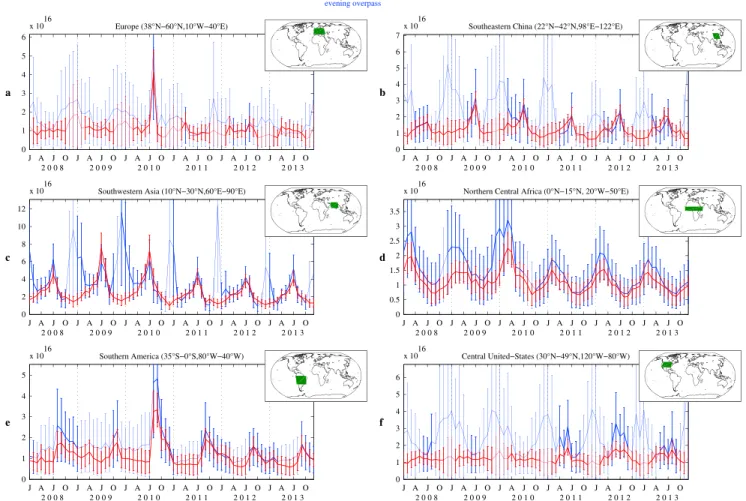
evening (right column) overpasses in Figure 1. The data correspond to weighted mean columns of the mea-surements performed during each season from 2008 to 2013 (0.25∘ × 0.5∘ cells); the resulting columns associated with a relative error above 75% have been filtered out, and the error distributions (not fil-tered) are shown as inset. These seasons are represented as 3 month periods: December-January-February (DJF, Figure 1, first row), March-April-May (MAM, second row), June-July-August (JJA, third row) and September-October-November (SON, fourth row). In Figure 2, we show the time evolution over the six years over six large areas, similar to the subcontinental boxes used by Shephard et al. [2011] (the six other regions are presented in the supporting information). Time series are shown separately for morning (red) and evening (blue) retrievals.
The seasonal distributions in Figure 1 together with the error maps highlight the varying sensitivity of IASI measurements for each region which makes the analyses of time series complex. It can be seen that the sensi-tivity is generally lower during the night (resulting in much larger error), due to less favorable thermal contrast, but that the main patterns are similar. On some occasions the measurements from the evening orbit concur in terms of sensitivity with those of the morning orbit (especially in case of temperature inversion [Clarisse
et al., 2010]), but this is not reflected in the seasonally aggregated distributions. Figure 2 shows further that
IASI observes a clear seasonality, which is different from one area to another. It is very important to consider the error bars to account for the variation in sensitivity as a function of month (and between orbits); only the
Figure 1. Composite seasonal distributions (molecules/cm2, vertical color bar) averaged over 6 years (1 January 2008 to 31 December 2013) of IASI-NH 3
(left column) morning and (right column) evening measurements in 0.25∘ ×0.5∘cells. (first to fourth rows) December-January-February (DJF), March-April-May (MAM), June-July-August (JJA), and September-October-November (SON) weighted mean distributions. A postfiltering consisting in excluding mean column values associated with a mean relative error above 75% has been applied. Relative weighted error distributions (%, not filtered, horizontal color bar) are presented as an inset in the bottom left corner of each seasonal map.
main patterns, identified in Figure 2 by thicker red and blue line (when the error is below 75%), are therefore discussed here. The retrieved columns from both overpasses follow in most cases a similar evolution, with overall higher evening columns associated with larger errors. Northern central Africa (Figure 2d) shows in particular a seasonal cycle fully captured by IASI daytime and nighttime measurements, with the latest columns being consistently larger than the daytime ones. This could be explained by the building-up of NH3
following emission during the day. Finally, in some regions, there are pronounced maxima in the evening mea-surements, which are absent in the morning ones. This is especially the case of southeastern China (Figure 2b) and southwestern Asia (Figure 2c), with the evening maxima observed in wintertime (see below).
In Europe (Figure 2a), the highest concentrations are measured in spring and summer (MAM and JJA, Figure 1) for the morning observations with maxima around 1.5×10¹⁶molecule/cm2. The stronger peak in August 2010,
Geophysical Research Letters
10.1002/2015GL065496
Figure 2. Monthly weighted time series of the NH3total columns (molecules/cm2) for the morning (red) and evening (blue) IASI overpasses covering the entire period from 1 January 2008 to 31 December 2013. Bold lines and error bars correspond to monthly means associated with a relative error below 75%. Each January is marked with a dashed vertical line, while thexaxis labels are January (J), April (A), July (J), and October (O); the different years are also indicated on the time axis. The subcontinental areas selected are similar to the ones from Shephard et al. [2011] and are indicated by green patches in the upper right corner inset map.
also clearly seen in the JJA distributions, is linked with the exceptional fires that occurred around Moscow that summer [Konovalov et al., 2011]. It emitted large amounts of NH3, which were transported to Central Europe
[R’Honi et al., 2013; Van Damme et al., 2015].
IASI measures large column values over several areas in Asia, with a maxima generally in July (well matching for morning and evening overpasses). These maxima are about twice as large for southwestern Asia (Figure 2c, around 4×10¹⁶ molecules/cm2) as compared to southeastern China (Figure 2b, around
2×10¹⁶molecules/cm2). The amplitudes of the cycle for southwestern Asia are also the largest of all regions
investigated, reaching 6.3×10¹⁶molecules/cm2between the minimum (December) and the maximum (July)
in 2010. For southeastern China, additional high monthly values (2×10¹⁶molecules/cm2) are observed in June
2012 and 2013. These summer peaks are consistent with several in situ data sets [Ianniello et al., 2010; Meng
et al., 2011; Shen et al., 2011]. Interestingly, for these two regions in Asia the measurements from the evening
orbit are for many months also associated with low errors. In winter, very high values are measured (up to 8–10×1016molecules/cm2in 2010 and 2011) possibly related to stable atmospheric conditions preventing
the dispersion of pollutants [Boynard et al., 2014]. Southwestern Asia is an area where IASI is able to probe NH3 throughout the year with relatively low error, with persistent highest columns in July, from 3.8×10¹⁶in 2012 up
to 7.5×10¹⁶molecules/cm2in 2009 during daytime and from 4.2×10¹⁶in 2012 up to 6.2×10¹⁶molecules/cm2
in 2010 during nighttime, with additional secondary peaks in December and/or January, mainly in the evening (especially in December 2009: 1.16×10¹⁷molecules/cm2). Note that from ground-based measurements, the
summer extrema for this part of the world have been reported around Delhi for 2011 by Singh and Kulshrestha [2012] and that high winter values have been also observed [Sharma et al., 2010].
In the central part of the African continent, high columns are retrieved in DJF and MAM for both morn-ing and evenmorn-ing overpasses. The northern central Africa region (Figure 2d) presents maxima in the range 1.5–2.5×10¹⁶molecules/cm2(slightly higher in the evening) in February. The entire cycle is captured and is
consistent with that observed by the IGAC/DEBITS/AFRICA (IDAF) ground-based network [Adon et al., 2010]. The southern part of this continent is characterized by lower columns peaking later in the year, in SON. In southern America (Figure 2e), the entire cycle is captured using the retrieved columns from the morning over-pass, while the nighttime measurements provide complementary information from August to January. The seasonality is characterized by enhanced NH3columns in JJA and SON with a persistent peak in September,
however, generally below 2×10¹⁶molecules/cm2. Higher columns over the 6 year period are reported in
August and September 2010, which is a year of exceptional burning [Chen et al., 2013].
As for Europe, the sensitivity of IASI to NH3in the North American continent is not always sufficient and the
total cycle cannot be perfectly characterized. From the morning-retrieved columns, we see that the values in Central U.S. (Figure 2f ) are larger in MAM and JJA. This is similar in Europe, but we observe that the U.S. summer values are closer to the spring values than in Europe. These observed temporal patterns are con-sistent with the ones reported by Pouliot et al. [2012] based on emission inventories. The minima (around 1×10¹⁶molecule/cm2) and maxima (around 1.5×10¹⁶molecule/cm2) are also pretty similar for these two
regions, possibly reflecting similarities in agricultural practices.
In comparison with the four (January, April, July, and October) monthly composite means provided by TES measurements [Shephard et al., 2011], we have shown with the discussion above that IASI is able to provide quantitative monthly resolved seasonal patterns, fluctuating each year depending on environmental condi-tions. The general patterns of seasonality inferred from IASI are broadly consistent with those reported by TES. Similar summer peaks are indeed observed for the Asian subcontinental areas, as well as high values during SON period in South America, and large NH3columns from December to April in North Central Africa.
3.2. Interannual Variability
The yearly global distributions from 2008 to 2013 are presented in the supporting information (Figure S1). These distributions are weighted means of all the measurements (morning and evening overpasses) per year included in each 0.25∘ latitude × 0.5∘ longitude cell. The year 2010 stands out from the other years due to the large biomass burning events which occurred in Russia and in southern America. Large agricultural areas such as the North China Plain, the Indo-Gangetic Plain, and the Great Plains in U.S. and Canada, exhibit high columns each year. Other persistent high signals are observed by IASI above biomass burning areas in West Africa, South America, and the boreal regions. A significant decrease of the NH3columns over West Africa is
observed in the years 2011–2013 (maximum column around 1.5–2×10¹⁶molecules/cm2), in comparison to
the years 2008–2010 (maximum column well above 2×10¹⁶molecules/cm2). This could be due to the strong
(2010–2011), moderate (2011–2012), and weak (2013) La Niña episodes [National Oceanic and Atmospheric
Administration, 2014], which cool this part of Africa, implying reduced NH3volatilization [Sutton et al., 2013]. An additional possible reason lies in the decrease of the savanna burning due to their conversion into crop-land [Andela and van der Werf , 2014]. Another decrease easily identifiable from the yearly global distributions occurs in North India, especially in the region including the Hindus and the Ganges Valleys. While character-izing the trends (see Figure S2 in the supporting information), we found statistically significant values only for the African regions and Australia. However, a longer time period of IASI-NH3observations and consistent
Level2 data are needed to confirm these first trend estimates.
3.3. Climatology of the Month of Maximum Columns
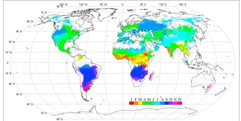
To explore the global variability in the timing of NH3maxima at a higher spatial resolution, a climatology map
of the monthly highest columns in 0.25∘ × 0.5∘ cells is presented in Figure 3, following an approach used earlier by van der A et al. [2008] for nitrogen dioxide (NO2). Monthly weighted means for each year based on
all morning and evening columns over the 6 year period have been used to draw this map. The composite monthly means for the six years have been subsequently calculated to determine the month with the highest column value. Due to their associated lower error estimates, the daytime observations are driving the resulting distribution. The error on the timing of the month of maximum columns has been estimated at 1 month by comparing the second and third maximum to the maximum (see supporting information Figure S3). Figure 3 highlights the timing diversity in NH3column maxima, which, if we neglect in first order the impact on
Geophysical Research Letters
10.1002/2015GL065496
Figure 3. Month of maximum NH3column determined in 0.25∘ ×0.5∘cells from NH3measurements performed between 1 January 2008 and 31 December 2013. Monthly weighted columns associated with a weighted relative error above 35% have been set to zero.
emissions of NOxand SO2), can be traced back to changes in emissions. It shows that a major part of
northwest-ern Europe has an April maximum, consistent with agricultural temporal emission pattnorthwest-erns for this area, which have a well-known associated spring peak due to fertilizer application [Friedrich and Reis, 2004; Paulot et al., 2014], and the fact that agriculture represents around 90% of NH3reported emissions in Europe [European
Environment Agency, 2014]. In contrast, southern Europe is characterized by June-July maxima and eastern
Europe by August maxima. Those summer southern European emission peaks are likely due to the enhanced NH3volatilization with increasing temperature [Sutton et al., 2013]. It is interesting to point out a well-marked autumn peak in Croatia and the Balkans, which could be related to vegetation fires. The August maxima for eastern Europe and part of Asia are highly consistent with the cycle of fire activity [Giglio et al., 2006], suggest-ing biomass burnsuggest-ing as a major source of NH3in these areas. These fires are generally caused by agricultural
burning, whereas the wildfires in boreal areas are responsible for the July peaks [Korontzi et al., 2006; Magi
et al., 2012].
In the northern part of southeastern Asia, IASI observes NH3column maxima in March and April (light green and yellow in Figure 3), while for the Indian subcontinent the peak month varies from February (southwest-ern India) to July (Pakistan and northeast(southwest-ern India). The detailed interpretation of these varying seasonal patterns on a relatively small continental scale is not straightforward considering the numerous emission processes simultaneously at work (e.g., fertilization, livestock, industry, agricultural, and domestic fires). For instance, the Indus basin is well known for its intensive agriculture based on large-scale irrigated crops [Land
Degradation Assessment in Drylands, 2013], and in that region fires do not seem to be responsible for the
observed peak in July. In contrast, the NH3maxima in southeastern Asia are well corresponding with the
sea-sonality of fires, which indicates that biomass burning is contributing significantly to the NH3columns [Giglio
et al., 2006]—except for Thailand where the peak in March suggests the dominance of agricultural sources.
The June-July peaks in the northern part and in particular in the North China Plain are likely linked with har-vest season associated with the intense burning of agricultural crop residues [Huang et al., 2012a]. The Sichuan province, characterized by high livestock densities [Huang et al., 2012b], has its highest values sooner in the year, in May (green).
Africa presents a high diversity in the months of NH3column maxima. The southern African continent is
The central and northern parts are much more variable with the peak month identified from January to August, pointing to mixed emission processes. In western Africa, and consistently with what is observed from ground-based measurement [Adon et al., 2010], NH3maxima are observed by IASI sooner above wet
savan-nas (February to April) than above dry savansavan-nas (May to July). This is interesting and tends to confirm the hypothesis of Delon et al. [2012] that dry savanna emissions are dominated by NH3volatilization (function
of soil temperature among others) while wet savanna emissions occur also because of burning processes. A 1 month lag is observed compared to the fire seasonality (peaking in January) for a large part of the northern central Africa, which suggests agricultural emissions following biomass burning, as recently proposed in
Whitburn et al. [2015].
The distribution of the month of maximum NH3in southern America is, as for the southern parts of Africa,
closely related with the fire seasonality (peaking from August to December), which indicates that this is the major source of NH3in this continent. As an example, the area peaking in August in Brazil is part of the “Arc
of Deforestation,” well known for its fire activity [Chen et al., 2013]. The maxima later in the year suggest NH3 emissions from agricultural areas, possibly linked with waste burning, especially in Argentina. The Llanos area (Venezuela) shows maxima in other months, March and April, which indicates that agricultural practices act there as a nonnegligible source, which add up to the vegetation burning that occurs primarily from January to March [Giglio et al., 2006].
In central and northern America, the spatial patterns in month of maximum columns are more homogeneous. Western U.S. is characterized by peaks in summer months, more than likely due to enhanced NH3 volatiliza-tion in a drier environment at higher temperature. Consistent high July-August NH3concentrations have, for
instance, been reported recently above a rural gas production area in western Wyoming [Li et al., 2014]. The San Joaquin Valley stands up in western U.S. showing its maximum of NH3columns in October. Further
stud-ies are needed to identify the reason for this difference, which could be related to the large weight associated with the evening measurements in that regions, indeed peaking in October-November [Clarisse et al., 2010]. The great plains in U.S. and Canada show an earlier maximum in April-May, suggesting agricultural spring emissions as a major source, similarly to Europe. The same can be said for Southern Ontario, in agreement with measurements from the ground [Zbieranowski and Aherne, 2013]. This timing is consistent with a study based on ammonium wet deposition data which have also shown this earlier peak of NH3for the Midwest region, attributed to differences in agricultural activities [Paulot et al., 2014].
4. Conclusions
We have analyzed 6 years (2008–2013) of NH3total columns retrieved globally from IASI measurements twice daily. Monthly mean total columns have been calculated with an error-weighting procedure for sev-eral regions, separately for morning and evening overpasses. In most situations, the monthly means from the IASI morning measurements have smaller errors. Despite this, the evening measurements allow capturing the seasonal cycle over northern central Africa as well; it highlights also additional winter peaks in southwestern Asia. In other regions, the evening measurements are not sufficiently accurate year-round, and for the months wherein measurements are available, a general consistency with the morning measurements is found. It is the first time that such an assessment of the added value of the evening IASI-NH3column observations is performed. It is also the first time that IASI-NH3observations are analyzed at subcontinental scale over a long period. It allows unprecedented investigations of the spatiotemporal variability of NH3in the atmosphere. The seasonal cycles are well marked in all regions, with the largest amplitude in Asia, where also the highest columns are measured (both at background and peak level). Europe’s and northern America’s seasonali-ties were categorized with a cycle of similar amplitude, characterized by high spring columns. The relations between atmospheric abundances and emission processes was also emphasized at smaller regional scale by extracting the global climatology of the month of maxima columns at high spatial resolution. In some regions, the predominance of a major source appears clearly (e.g., agriculture in Europe and north America and fires in central South Africa and south America), while in others mixed source processes on small scale are obvi-ous (e.g., northern central Africa and southwestern Asia). We finally demonstrated that while the interannual variability does not allow to reveal clear trends, 2010 stands up as the year with largest NH3concentrations,
principally because of large emissions from fires in both hemispheres.
More generally, the results presented here underline the significance of the IASI satellite measurements of NH3, which are performed at high temporal sampling and resolution, to characterize and understand the
Geophysical Research Letters
10.1002/2015GL065496
variability of sources and atmospheric processes on the globe and thereby to help constraining models in the parameterization of these processes, as a function of environmental conditions and anthropogenic prac-tices. In particular, the multiyear data set available from IASI satellites will allow, with the help of global chemistry-transport models, to assess bottom-up emission inventories through source inversion and to improve on our knowledge of area-specific emission seasonality and interannual variability. It will also allow examining the effect of other changing geophysical or climatic parameters (temperature and NO2or SO2
emissions) on the NH3global distributions.
References
Adon, M., et al. (2010), Long term measurements of sulfur dioxide, nitrogen dioxide, ammonia, nitric acid and ozone in Africa using passive samplers, Atmos. Chem. Phys., 10(15), 7467–7487, doi:10.5194/acp-10-7467-2010.
Andela, N., and G. R. van der Werf (2014), Recent trends in African fires driven by cropland expansion and El Niño to La Niña transition,
Nat. Clim. Change, 4(9), 791–795, doi:10.1038/nclimate2313.
August, T., D. Klaes, P. Schlüssel, T. Hultberg, M. Crapeau, A. Arriaga, A. O’Carroll, D. Coppens, R. Munro, and X. Calbet (2012), IASI on Metop-A: Operational Level 2 retrievals after five years in orbit, J. Quant. Spectrosc. Radiat. Transfer, 113(11), 1340–1371, doi:10.1016/j.jqsrt.2012.02.028.
Bobbink, R., et al. (2010), Global assessment of nitrogen deposition effects on terrestrial plant diversity: A synthesis, Ecol. Appl., 20(1), 30–59, doi:10.1890/08-1140.1.
Bouwman, A. F., L. J. M. Boumans, and N. H. Batjes (2002), Estimation of global NH3volatilization loss from synthetic fertilizers and animal manure applied to arable lands and grasslands, Global Biogeochem. Cycles, 16(2), 1024, doi:10.1029/2000GB001389.
Boynard, A., et al. (2014), First simultaneous space measurements of atmospheric pollutants in the boundary layer from IASI: A case study in the North China Plain, Geophys. Res. Lett., 41, 645–651, doi:10.1002/2013GL058333.
Chen, Y., D. C. Morton, Y. Jin, G. J. Collatz, P. S. Kasibhatla, G. R. van der Werf, R. S. DeFries, and J. T. Randerson (2013), Long-term trends and interannual variability of forest, savanna and agricultural fires in South America, Carbon Manage., 4(6), 617–638, doi:10.4155/cmt.13.61. Clarisse, L., C. Clerbaux, F. Dentener, D. Hurtmans, and P.-F. Coheur (2009), Global ammonia distribution derived from infrared satellite
observations, Nat. Geosci., 2(7), 479–483, doi:10.1038/ngeo551.
Clarisse, L., M. Shephard, F. Dentener, D. Hurtmans, K. Cady-Pereira, F. Karagulian, M. Van Damme, C. Clerbaux, and P.-F. Coheur (2010), Satellite monitoring of ammonia: A case study of the San Joaquin Valley, J. Geophys. Res., 115, D13302, doi:10.1029/2009JD013291. Clerbaux, C., et al. (2009), Monitoring of atmospheric composition using the thermal infrared IASI/MetOp sounder, Atmos. Chem. Phys.,
9(16), 6041–6054, doi:10.5194/acp-9-6041-2009.
Delon, C., C. Galy-Lacaux, M. Adon, C. Liousse, D. Serça, B. Diop, and A. Akpo (2012), Nitrogen compounds emission and deposition in West African ecosystems: Comparison between wet and dry savanna, Biogeosciences, 9(1), 385–402, doi:10.5194/bg-9-385-2012.
Emission Database for Global Atmospheric Research (2014), EDGAR Version 4.2. Source: EC-JRC/PBL. [Available at http://edgar.jrc.ec.europa.eu, last access: 15 December 2012.]
European Environment Agency (2014), Effects of air pollution on European ecosystems: Past and future exposure of European freshwater and terrestrial habitats to acidifying and eutrophying air pollutants. [Available at http://www.eea.europa.eu/data-and-maps/ indicators/eea-32-ammonia-nh3-emissions-1/assessment-2, last access: 20 August 2013.]
Erisman, J. W., A. Bleeker, J. Galloway, and M. Sutton (2007), Reduced nitrogen in ecology and the environment, Environ. Pollut., 150(1), 140–149, doi:10.1016/j.envpol.2007.06.033.
Erisman, J. W., J. N. Galloway, S. Seitzinger, A. Bleeker, N. B. Dise, A. M. R. Petrescu, A. M. Leach, and W. de Vries (2013), Consequences of human modification of the global nitrogen cycle, Philos. Trans. R. Soc. B, 368(1621), 20130116, doi:10.1098/rstb.2013.0116. Friedrich, R., and S. Reis (Eds.) (2004), Emissions of Air Pollutants: Measurements, Calculations and Uncertainties, Springer, Berlin, and
New York.
Giglio, L., I. Csiszar, and C. O. Justice (2006), Global distribution and seasonality of active fires as observed with the Terra and Aqua Moderate Resolution Imaging Spectroradiometer (MODIS) sensors, J. Geophys. Res., 111, G02016, doi:10.1029/2005JG000142.
Gilliland, A. B., R. L. Dennis, S. J. Roselle, and T. E. Pierce (2003), Seasonal NH3emission estimates for the eastern United States based on
ammonium wet concentrations and an inverse modeling method, J. Geophys. Res., 108(D15), 4477, doi:10.1029/2002JD003063. Gilliland, A. B., K. W. Appel, R. W. Pinder, and R. L. Dennis (2006), Seasonal NH3emissions for the continental United States: Inverse model
estimation and evaluation, Atmos. Environ., 40(26), 4986–4998, doi:10.1016/j.atmosenv.2005.12.066.
Gu, B., M. A. Sutton, S. X. Chang, Y. Ge, and J. Chang (2014), Agricultural ammonia emissions contribute to China’s urban air pollution,
Front. Ecol. Environ., 12(5), 265–266, doi:10.1890/14.WB.007.
Heald, C. L., et al. (2012), Atmospheric ammonia and particulate inorganic nitrogen over the United States, Atmos. Chem. Phys., 12(21), 10,295–10,312, doi:10.5194/acp-12-10295-2012.
Huang, X., Y. Song, M. Li, J. Li, and T. Zhu (2012a), Harvest season, high polluted season in East China, Environ. Res. Lett., 7(4), 044033, doi:10.1088/1748–9326/7/044033.
Huang, X., Y. Song, M. Li, J. Li, Q. Huo, X. Cai, T. Zhu, M. Hu, and H. Zhang (2012b), A high-resolution ammonia emission inventory in China,
Global Biogeochem. Cycles, 26, GB1030, doi:10.1029/2011GB004161.
Ianniello, A., F. Spataro, G. Esposito, I. Allegrini, E. Rantica, M. P. Ancora, M. Hu, and T. Zhu (2010), Occurrence of gas phase ammonia in the area of Beijing (China), Atmos. Chem. Phys., 10(19), 9487–9503, doi:10.5194/acp-10-9487-2010.
Konovalov, I. B., M. Beekmann, I. N. Kuznetsova, A. Yurova, and A. M. Zvyagintsev (2011), Atmospheric impacts of the 2010 Russian wildfires: Integrating modelling and measurements of an extreme air pollution episode in the Moscow region, Atmos. Chem. Phys.,
11(19), 10,031–10,056, doi:10.5194/acp-11-10031-2011.
Korontzi, S., J. McCarty, T. Loboda, S. Kumar, and C. Justice (2006), Global distribution of agricultural fires in croplands from 3 years of Moderate Resolution Imaging Spectroradiometer (MODIS) data, Global Biogeochem. Cycles, 20, GB2021, doi:10.1029/2005GB002529. Land Degradation Assessment in Drylands (2013), Mapping land use systems at global and regional scales for land degradation assessment
analysis, Tech. Rep. 8, v1.1.
Li, Y., et al. (2014), Observations of ammonia, nitric acid, and fine particles in a rural gas production region, Atmos. Environ., 83, 80–89, doi:10.1016/j.atmosenv.2013.10.007.
Magi, B. I., S. Rabin, E. Shevliakova, and S. Pacala (2012), Separating agricultural and non-agricultural fire seasonality at regional scales,
Biogeosciences, 9(8), 3003–3012, doi:10.5194/bg-9-3003-2012.
Acknowledgments
The IASI-NH3observations are available on request at ULB. IASI has been developed and built under the responsibility of the “Centre National d’Etudes Spatiales” (CNES, France). It is flown on board the MetOp satellites as part of the EUMETSAT Polar System. The IASI L1 data are received through the EUMETCast near-real-time data distribution service. The research in Belgium was funded by the F.R.S.-FNRS, the Belgian State Federal Office for Scientific, Technical and Cultural Affairs (Prodex arrangement 4000111403 IASI.FLOW). M. Van Damme and S. Whitburn are grateful to the “Fonds pour la Formation à la Recherche dans l’Industrie et dans l’Agriculture” of Belgium for a PhD grant (Boursier FRIA). L. Clarisse and P.-F. Coheur are, respectively, Research Associate and Senior Research Associate with F.R.S.-FNRS. C. Clerbaux is grateful to CNES for scientific collaboration and financial support. We gratefully acknowledge support from the project “Effects of Climate Change on Air Pollution Impacts and Response Strategies for European Ecosystems” (ÉCLAIRE), funded under the EC Seventh Framework Programme (grant agreement 282910). Part of this research was supported by the EC under the Seventh Framework Programme (grant agreement 606719), for the project “Partnership with China on Space Data (PANDA).” We also would like to thank J. Hadji-Lazaro and C. Wespes for their assistance and the reviewers for their useful comments.
The Editor thanks two anonymous reviewers for their assistance in evaluating this paper.
Meng, Z. Y., W. L. Lin, X. M. Jiang, P. Yan, Y. Wang, Y. M. Zhang, X. F. Jia, and X. L. Yu (2011), Characteristics of atmospheric ammonia over Beijing, China, Atmos. Chem. Phys., 11(12), 6139–6151, doi:10.5194/acp-11-6139-2011.
National Oceanic and Atmospheric Administration (2014), National Weather Services—Cold and Warm Episodes by Season. [Availble at http://www.cpc.noaa.gov/products/analysis_monitoring/ensostuff/ensoyears.shtml, last access: 2 November 2014.]
Paerl, H. W., W. S. Gardner, M. J. McCarthy, B. L. Peierls, and S. W. Wilhelm (2014), Algal blooms: Noteworthy nitrogen, Science, 346(6206), 175, doi:10.1126/science.346.6206.175-a.
Paulot, F., and D. J. Jacob (2014), Hidden cost of U.S. agricultural exports: Particulate matter from ammonia emissions, Environ. Sci. Technol.,
48(2), 903–908, doi:10.1021/es4034793.
Paulot, F., D. J. Jacob, R. W. Pinder, J. O. Bash, K. Travis, and D. K. Henze (2014), Ammonia emissions in the United States, European Union, and China derived by high-resolution inversion of ammonium wet deposition data: Interpretation with a new agricultural emissions inventory (MASAGE_NH3), J. Geophys. Res. Atmos., 119, 4343–4364, doi:10.1002/2013JD021130.
Pinder, R. W., J. T. Walker, J. O. Bash, K. E. Cady-Pereira, D. K. Henze, M. Luo, G. B. Osterman, and M. W. Shephard (2011), Quantifying spatial and seasonal variability in atmospheric ammonia with in situ and space-based observations, Geophys. Res. Lett., 38, L04802, doi:10.1029/2010GL046146.
Pope, C. A. I., M. Ezzati, and D. W. Dockery (2009), Fine-particulate air pollution and life expectancy in the United States, N. Engl. J. Med.,
360(4), 376–386, doi:10.1056/NEJMsa0805646.
Pouliot, G., T. Pierce, H. D. van der Gon, M. Schaap, M. Moran, and U. Nopmongcol (2012), Comparing emission inventories and model-ready emission datasets between Europe and North America for the AQMEII project, Atmos. Environ., 53, 4–14, doi:10.1016/j.atmosenv.2011.12.041.
R’Honi, Y., L. Clarisse, C. Clerbaux, D. Hurtmans, V. Duflot, S. Turquety, Y. Ngadi, and P.-F. Coheur (2013), Exceptional emissions of NH3and HCOOH in the 2010 Russian wildfires, Atmos. Chem. Phys., 13(8), 4171–4181, doi:10.5194/acp-13-4171-2013.
Sharma, S., A. Datta, T. Saud, M. Saxena, T. Mandal, Y. Ahammed, and B. Arya (2010), Seasonal variability of ambient NH3, NO, NO2and SO2 over Delhi, J. Environ. Sci., 22(7), 1023–1028, doi:10.1016/S1001-0742(09)60213-8.
Shen, J., X. Liu, Y. Zhang, A. Fangmeier, K. Goulding, and F. Zhang (2011), Atmospheric ammonia and particulate ammonium from agricultural sources in the North China Plain, Atmos. Environ., 45(28), 5033–5041, doi:10.1016/j.atmosenv.2011.02.031.
Shephard, M. W., et al. (2011), TES ammonia retrieval strategy and global observations of the spatial and seasonal variability of ammonia,
Atmos. Chem. Phys., 11(20), 10,743–10,763, doi:10.5194/acp-11-10743-2011.
Singh, S., and U. C. Kulshrestha (2012), Abundance and distribution of gaseous ammonia and particulate ammonium at Delhi, India,
Biogeosciences, 9(12), 5023–5029, doi:10.5194/bg-9-5023-2012.
Sutton, M. A., et al. (2007), Challenges in quantifying biosphere-atmosphere exchange of nitrogen species, Environ. Pollut., 150(1), 125–139, doi:10.1016/j.envpol.2007.04.014.
Sutton, M. A., et al. (2013), Towards a climate-dependent paradigm of ammonia emission and deposition, Philos. Trans. R. Soc. B, 368(1621), 20130166, doi:10.1098/rstb.2013.0166.
Van Damme, M., L. Clarisse, C. L. Heald, D. Hurtmans, Y. Ngadi, C. Clerbaux, A. J. Dolman, J. W. Erisman, and P. F. Coheur (2014a), Global distri-butions, time series and error characterization of atmospheric ammonia (NH3) from IASI satellite observations, Atmos. Chem. Phys., 14(6),
2905–2922, doi:10.5194/acp-14-2905-2014.
Van Damme, M., R. J. Wichink Kruit, M. Schaap, L. Clarisse, C. Clerbaux, P.-F. Coheur, E. Dammers, A. J. Dolman, and J. W. Erisman (2014b), Evaluating four years of atmospheric ammonia (NH3) over Europe using IASI satellite observations and LOTOS-EUROS model results,
J. Geophys. Res. Atmos., 119, 9549–9566, doi:10.1002/2014JD021911.
Van Damme, M., et al. (2015), Towards validation of ammonia (NH3) measurements from the IASI satellite, Atmos. Meas. Tech., 8(3), 1575–1591, doi:10.5194/amt-8-1575-2015.
van der A, R. J., H. J. Eskes, K. F. Boersma, T. P. C. van Noije, M. Van Roozendael, I. De Smedt, D. H. M. U. Peters, and E. W. Meijer (2008), Trends, seasonal variability and dominant NOxsource derived from a ten year record of NO2measured from space, J. Geophys. Res., 113, D04302, doi:10.1029/2007JD009021.
Whitburn, S., M. Van Damme, J. Kaiser, G. van der Werf, S. Turquety, D. Hurtmans, L. Clarisse, C. Clerbaux, and P. F. Coheur (2015), Ammonia emissions in tropical biomass burning regions: Comparison between satellite-derived emissions and bottom-up fire inventories,
Atmos. Environ., doi:10.1016/j.atmosenv.2015.03.015.
Wichink Kruit, R. J., M. Schaap, F. J. Sauter, M. C. van Zanten, and W. A. J. van Pul (2012), Modeling the distribution of ammonia across Europe including bi-directional surface-atmosphere exchange, Biogeosciences, 9(12), 5261–5277, doi:10.5194/bg-9-5261-2012.
Zbieranowski, A. L., and J. Aherne (2013), Ambient concentrations of atmospheric ammonia, nitrogen dioxide and nitric acid in an intensive agricultural region, Atmos. Environ., 70, 289–299, doi:10.1016/j.atmosenv.2013.01.023.