HAL Id: hal-01510642
https://hal.sorbonne-universite.fr/hal-01510642
Submitted on 19 Apr 2017HAL is a multi-disciplinary open access archive for the deposit and dissemination of sci-entific research documents, whether they are pub-lished or not. The documents may come from teaching and research institutions in France or abroad, or from public or private research centers.
L’archive ouverte pluridisciplinaire HAL, est destinée au dépôt et à la diffusion de documents scientifiques de niveau recherche, publiés ou non, émanant des établissements d’enseignement et de recherche français ou étrangers, des laboratoires publics ou privés.
Landscape features impact connectivity between soil
populations: a comparative study of gene flow in
earthworms
L. Dupont, M. Torres-Leguizamon, P. René-Corail, J. Mathieu
To cite this version:
L. Dupont, M. Torres-Leguizamon, P. René-Corail, J. Mathieu. Landscape features impact connec-tivity between soil populations: a comparative study of gene flow in earthworms. Molecular Ecology, Wiley, 2017, 26 (12), pp.3128 - 3140. �10.1111/mec.14102�. �hal-01510642�
Landscape features impact connectivity between soil populations: a comparative study 1
of gene flow in earthworms 2
3
L. Dupont1*, M. Torres-Leguizamon1, P. René-Corail1 and J. Mathieu2 4
5 1
Université Paris Est Créteil (UPEC), UPMC, Paris 7, CNRS, INRA, IRD, Institut d’écologie 6
et des sciences de l’environnement de Paris, 94010 Créteil Cedex, France 7
2
Sorbonne Universités, UPMC Univ Paris 06, UPEC, Paris 7, CNRS, INRA, IRD, Institut 8
d’Ecologie et des Sciences de l’Environnement de Paris, 75005, Paris, France 9
10
* Corresponding author. Tel : +33(0)145171664 ; Fax : +33(0)145171999 ; e-mail address : 11
lise.dupont@u-pec.fr 12
13
14
Key-Words : Dispersal, genetic diversity, genetic structure, landscape connectivity, local 15
landscape structure, microsatellites 16
17
Running Title : Landscape genetics of earthworms 18
19
Abstract 21
22
Landscape features are known to alter the spatial genetic variation of above ground 23
organisms. Here, we tested the hypothesis that the genetic structure of below ground 24
organisms also responds to landscape structure. Microsatellite markers were used to carry out 25
a landscape genetic study of two endogeic earthworm species, Allolobophora chlorotica (N = 26
440, 8 microsatellites) and Aporrectodea icterica (N = 519, 7 microsatellites), in an 27
agricultural landscape in the North of France, where landscape features were characterised 28
with high accuracy. We found that habitat fragmentation impacted genetic variation of 29
earthworm populations at the local scale. A significant relationship was observed between 30
genetic diversity (He, Ar) and several landscape features in A. icterica populations and A. 31
chlorotica. Moreover, a strong genetic differentiation between sites was observed in both 32
species, with a low degree of genetic admixture and high Fst values. The landscape 33
connectivity analysis (MLPE) at the regional scale, including Isolation By Distance (IBD), 34
Least Cost Path (LCP) and Cost Weighted Distance (CWD) approaches, showed that genetic 35
distances were linked to landscape connectivity in A. chlorotica. This indicates that the 36
fragmentation of natural habitats has shaped their dispersal patterns and local effective 37
population sizes. Landscape connectivity analysis confirmed that a priori favourable habitats 38
such as grasslands may constitute dispersal corridors for these species. 39
Introduction 41
42
A number of studies showed that spatial genetic variations of aboveground organisms 43
respond to changes in their landscape, through mechanisms involving movements of 44
organisms (review in Storfer et al. 2010; Manel & Holderegger 2013; Hall & Beissinger 45
2014). It is now well established that landscape features alter aboveground organisms' genetic 46
structure. Comparatively little is known about the impact of landscape-scale habitat 47
heterogeneity on belowground organisms, such as soil invertebrates, whose mobility is more 48
restricted (Vanbergen et al. 2007). Despite their importance in ecosystem functioning and in 49
the delivery of many ecosystem services (Lavelle et al. 1997; Jouquet et al. 2006; Lavelle et 50
al. 2006; Blouin et al. 2013), we still do not have a grasp of even basic information about 51
population genetic structure of soil organisms. For instance, Costa et al. (2013) found only 52
sixteen different species among the collembolans, earthworms and isopods groups of soil 53
invertebrates for which a population genetics study was carried out. Some of these papers 54
investigated the spatial genetic structure of soil organisms at a fine-scale (Sullivan et al. 2009; 55
Novo et al. 2010; Dupont et al. 2015), but none addressed the effect of landscape features on 56
genetic variation. However, terrestrial habitat heterogeneity is known to affect the diversity of 57
soil species’ assemblages by producing variation in the diversity of plant and litter 58
(Vanbergen et al. 2007). It is therefore assumed that aboveground structure and diversity 59
could profoundly impact the population genetic structure of belowground organisms. 60
61
The methodology of landscape genetics allows one to test the influence of the landscape 62
and environmental characteristics on microevolutionary processes and metapopulation 63
dynamics, including gene flow and local adaptation (Manel et al. 2003; Storfer et al. 2007; 64
Holderegger & Wagner 2008). Landscape connectivity is a twofold parameter made up of 65
structural connectivity and functional connectivity. Structural connectivity refers to the 66
physical relationship between landscape elements while functional connectivity may be 67
defined as the ease with which a lanscape can be crossed by an organism (Taylor et al. 2006). 68
Depending on the organisms, the permeability of the landscape will differ and some 69
constituent elements of the landscape can facilitate dispersal (i.e. “corridors”) while others 70
can impede or reduce the passage of dispersers (i.e. “barriers”) (Taylor et al. 1993). 71
Landscape structure can also have an important effect on passive dispersers by altering the 72
abiotic and biotic conditions that affect movement (Matthysen 2012). In order to understand 73
how landscape characteristics influence functional connectivity, resistance surfaces are 74
usually constructed and translated into measures of inter-population connectivity principally 75
using two kinds of models. Least-cost path models (Adriaensen et al. 2003) assume that 76
movement or gene flow rates between each pair of sites is related to the total cumulative 77
resistance or ‘cost’ (sum of per-pixel resistance values) along a single optimal path, while 78
circuit-theory based models (McRae 2006) incorporate all possible pathways across 79
landscapes, and their parameters and predictions can be expressed in terms of random walk 80
probabilities (Cost Weighted Distance "CWD", or "resistance approach"). Spear et al. (2010) 81
highlighted that both models provide complementary indices of connectivity with Least-cost-82
path distances being more informative at local scales and circuit theoretic models being 83
particularly useful for incorporating effects of gene flow over multiple generations. 84
85
Here, we were interested in landscape features impacting genetic variation and functional 86
connectivity in earthworms. Dispersal by passive mechanisms, such as zoochory, wind, water 87
and human activities is believed to be implicated in their long-distance movement (Eijsackers 88
2011; Costa et al. 2013; Dupont et al. 2015), whilst their active dispersal is dependent on 89
habitat quality, conspecific density, and habitat modification by conspecifics in endogeic (i.e. 90
species living in the upper organo-mineral soil layers and forming horizontal non-permanent 91
burrows, Bouché 1977) and anecic (i.e. species forming permanent or semi-permanent 92
vertical burrows in the soil which open at the surface where the earthworm emerges to feed, 93
Bouché 1977) species (Mathieu et al. 2010; Caro et al. 2012; Caro et al. 2013). The 94
distribution of these restricted dispersers is known to be controlled by soil parameters at the 95
field scale and by land use (forest, grassland and agricultural field), soil management, soil 96
type and climatic conditions at scales exceeding the field level; studies at the landscape scale 97
are thus challenging since fine-scale heterogeneity as well as gradients affecting regional-98
scale patterns have to be accounted for (Palm et al. 2013). 99
In order to investigate whether landscape features impact the genetic structure of 100
earthworm populations, we carried out a regional-scale comparative survey of genetic 101
variation in two species commonly found in European agricultural landscapes, the green 102
morph of Allolobophora chlorotica (Savigny, 1826) and Aporrectodea icterica (Savigny, 103
1826). Both species are endogeic but present several ecological differences. A. chlorotica 104
typically lives between soil surface and the upper 60 mm soil layer (Sims & Gerard 1999) and 105
is theoretically able to travel over 167 m per year in constant suitable conditions (Caro et al. 106
2013). However, in the field, dispersal distances ranging from 6.82 to 7.56m per year were 107
estimated in a recent population genetics study at fine spatial scales (Dupont et al. 2015). A. 108
icterica is found deeper in soils and is considered to be more mobile, being theoretically able 109
to travel up to 500 m.year-1 under constant artificial conditions (Mathieu et al. 2010; Caro et 110
al. 2013). An extremely low signal of genetic structure was obtained for this species in a fine-111
scale population genetics study at the within plot scale (100x80m). This result was explained 112
by the great dispersal capacity of the species (Dupont et al. 2015). Moreover, no pattern of 113
isolation by distance (IBD, i.e. decrease in the genetic similarity among populations as the 114
geographic distance between them increases) was observed among six A. icterica populations 115
separated by less than 13km (Torres-Leguizamon et al. 2014). 116
We analysed the relationship between landscape features and genetic variation in these 117
two common earthworm species, at fine and regional scales (Fig. 1), in an agricultural 118
landscape in North of France, where both species are common (e.g. Richard et al. 2012). First, 119
we tested the hypothesis that the mosaic of habitats created by anthropogenic drivers alters the 120
genetic diversity in earthworm populations using a buffer approach. This approach consists in 121
assessing the correlation between the genetic variation of the earthworm population and the 122
local landscape structure. Second, we tested the hypothesis that the different elements of the 123
landscape could act either as dispersal barriers or corridors for earthworms with a landscape 124
connectivity analysis at the regional scale (Zeller et al. 2012), encompassing Isolation by 125
Distance (IBD), Least Cost Path (LCP) and resistance (CWD) approaches. The role of three 126
elements, i.e. grasslands, crops and roads, was specifically tested. Grassland represents a 127
suitable habitat that could be easily crossed by endogeic species (Bouché 1972; Decaens et al. 128
2008) while soil tillage and the use of pesticides in cultivated soils are known to have a 129
detrimental effect on earthworms (Bertrand et al. 2015) and roads have been shown to 130
represent dispersal corridors for invasive earthworms (Cameron & Bayne 2009). 131
Material and Methods 133
134
Study Area and Sampling
135
Earthworms were collected in Normandy (northern France, Fig. 2) in 2009 and 2010. 136
The first sampling campaign was carried out in March and April 2009 in two pastures (PA and 137
PB) ~ 500m apart at the local agricultural school “Lycée Agricole d’Yvetot”. Details of these 138
sampling sites and methods are given in Dupont et al. (2015). The second sampling campaign 139
was carried out in April 2010, during which 39 other pastures were prospected. A. chlorotica 140
and A. icterica were found in 14 and 19 pastures, respectively (Fig. 2 and Table 1). We 141
selected pastures that had similar management histories, in order to reduce the effect of local 142
environmental variations. The location of the plots was chosen in order to maximise the 143
normality of the pairwise distance between plots. All pastures were at least 5 years old, and 144
the great majority was grazed by cattle. Within each plot of 10 x 10m, 30 individuals were 145
captured by sampling five monoliths of soil (25 x 25cm x 30 cm deep). If a species was 146
present in the samples of a plot, but less than 30 individuals were captured, we sampled other 147
monoliths - less than 10 m apart from the others- until the target of 30 individuals per 148
population was reached. Individuals were preserved in pure ethanol for DNA analysis. 149
150
DNA extraction, microsatellite genotyping and basic genetic statistics
151
Total genomic DNA of A. icterica was extracted using either the CTAB extraction 152
protocol, as described in Torres-Leguizamon et al. (2014) or the DNeasy 96 Blood & Tissue 153
Kit (Quiagen). The latter was also used for A. chlorotica. 154
A. chlorotica individuals were genotyped at the eight microsatellite loci described in 155
Dupont et al. (2011) while A. icterica individuals were genotyped at seven microsatellite loci 156
described in Torres-Leguizamon et al. (2012) and Dupont et al. (2015). Loci were amplified 157
by polymerase chain reaction (PCR) following protocols detailed in Dupont et al. (2011), 158
Torres-Leguizamon et al. (2012) and Dupont et al. (2015). The migration of PCR products 159
was carried out on a 3130xl Genetic Analyser using the LIZ500 size standard, alleles were 160
scored using GENESCAN V3.7 and GENOTYPER V3.7 software (Applied Biosystems, 161
Foster City, CA, USA). 162
Individuals missing 3 or more loci (e.g. failed PCR, poor-quality DNA extract) were 163
excluded from our dataset and ambiguous PCR results were duplicated. Mean genotyping 164
error rates per locus and per allele (Pompanon et al. 2005) were estimated from repeat 165
genotyping of 5% of samples (24 individuals per species). The null hypothesis of 166
independence between loci was tested from statistical genotypic disequilibrium analysis using 167
GENEPOP v. 4.4 (Rousset 2008). Evidence of null alleles was examined using the software 168
MICRO-CHECKER (Van Oosterhout et al. 2004) and from the frequency of null homozygote 169
within populations. The statistical power to detect genetic divergence was measured for all the 170
samples and markers using POWSIM 4.0 to evaluate the hypothesis of genetic homogeneity 171
under Fisher’s exact tests (Ryman & Palm 2006). Microsatellite loci were tested for departure 172
from Hardy–Weinberg equilibrium (HWE) within each sampling population using exact tests 173
implemented in GENEPOP v. 4.4. To adjust for multiple comparisons, the FDR method 174
(Benjamini & Hochberg 1995) as implemented in the software SGoF 175
(http://webs.uvigo.es/acraaj/SGoF.htm) was applied. 176
177
Genetic variation of earthworm populations
178
For each population, the genetic diversity was analysed by computing allelic richness 179
standardized for sample size (Ar; N= 26 and N = 9 for A. chlorotica and A. icterica 180
respectively) using the program FSTAT v2.9.3.2 (Goudet 2000) and expected heterozygosity 181
(He) using Genetix v 4.05 (Belkhir et al. 2004). Weir and Cockerham’s (1984) estimator of 182
the inbreeding coefficient Fis was calculated using GENEPOP v. 4.4 (Rousset 2008). The 183
distribution of the genetic diversity within populations can diverge from equilibrium models 184
due to demographic changes. We tested whether the populations recently experienced a 185
reduction of their effective size using the approach detailed in Cornuet & Luikart (1996) and 186
implemented in their software BOTTLENECK v. 1.2.02. Using a Wilcoxon test, the observed 187
heterozygosity was compared with the heterozygosity expected under equilibrium, 188
considering a two-phase mutation model (TPM) recommended for microsatellite data (Piry et 189
al. 1999) with 90% single-step mutations and 10% multiple-step mutations (and a variance 190
among multiple step of 12). Populations exhibiting a significant heterozygosity excess would 191
be considered as having experienced a recent genetic bottleneck whereas populations that 192
have been expanding for many generations are characterized by loci exhibiting a 193
heterozygosity deficiency (Cornuet & Luikart 1996). 194
We estimated genetic differentiation between populations by calculating Weir and 195
Cockerham’s (1984) estimator of pairwise Fst values and carrying out exact tests of allelic 196
differentiation between populations using GENEPOP v.4.0. To adjust for multiple 197
comparisons, the FDR correction was used. Due to the frequent presence of null alleles, we 198
used the program FREENA to calculate pairwise Fst estimates corrected for null alleles 199
(Fst_COR) using the so-called ENA method (Chapuis & Estoup 2007). This software was also 200
used to estimate the Cavalli-Sforza and Edwards (1967) genetic distance for each pair of 201
populations (Dc) and this distance was also estimated using the INA correction described in 202
Chapuis and Estoup (Dc_COR, 2007). Matrices of pairwise genetic distances were compared 203
with Mantel tests (Mantel 1967) using the R program (R Development Core Team 2012). 204
We used the program BAPS v.6 (Corander & Marttinen 2006; Corander et al. 2008) to 205
detect clusters of genetically similar populations and to estimate individual coefficients of 206
ancestry with regard to the detected clusters. When testing for population clusters, we ran 5 207
replicates for k = 5, k= 10, k= 15, k= 20, k= 25 and k=30, where k is the maximum number of 208
genetically divergent groups (populations). When estimating individual ancestry coefficients 209
via admixture analysis we used recommended values of (i) the number of iterations used to 210
estimate the admixture coefficients for the individuals (100), (ii) the number of reference 211
individuals from each population (200) and (iii) the number of iterations used to estimate the 212
admixture coefficients for the reference individuals (20). 213
214
Landscape genetics
215
Landscape elements were mapped at high resolution (precision ~2m) over the whole 216
area. Land use cover and linear elements such as roads and rivers were obtained by merging 217
different sources of data. As background data, we used databases from the French National 218
Geographic Institute (IGN), encompassing shapefiles (BD TOPO, accuracy ~1m), and raster 219
(BD Ortho, resolution = 0.5m) of the year 2010. We crossed this information with field work 220
with a differential GPS with 10 cm real time accuracy, in order to check the boundaries of 221
plots and their management. We also compared our data with Corine Land cover 2006 to 222
identify any inconsistencies. Historical and management information was gained with google 223
maps, from interviews with the farmers, and checked with the different version of Corine 224
Land Cover. The data base and the different geographical layers were built up in ArcGis 10.1 225
(ESRI) in the projection Lambert 93 (EPSG: 2154). Data were stored in a vector format and 226
rasterized at 10m resolution in order to perform the landscape analysis. Polygons and linear 227
elements were rasterized separately and merged in raster format. Linear elements were 228
buffered before rasterization in order to avoid artefact gaps. Landscape structure variables 229
were computed in Fragstats (McGarigal et al. 2012) and were computed at patch scale or at 230
the buffer scale (500m of radius) depending on the metric. Landscape descriptors were then 231
normalized (centred and reduced) and selected for the statistical modelling process based on 232
their Variance Inflation Factor value (VIF), in order to avoid collinearity. There is no 233
theoretical base to choose the threshold of the VIF value to exclude variables, and it is usually 234
recommended to use a predictors with a VIF below ten (Montgomery & Peck 1992; Zuur et 235
al. 2010; Dormann et al. 2013). We used a threshold of six in this study. Landscape structure 236
descriptors were correlated to genetic diversity indices (Ar, He) with multiple regression. In 237
order to select the best model, we run all combinations of factors and selected the model with 238
the best weight, based on corrected AIC (AICc) criteria. This approach produces r2 goodness 239
of fit and avoids over-fitting, thanks to the AIC criteria. 240
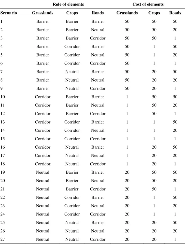
Landscape connectivity was performed by defining different scenarios of cost of 241
movements within landscape elements, based on species ecology. Elements were classified in 242
three categories: Barrier, Neutral or Corridors, which corresponded to decreasing movement 243
cost (50, 20, 1 respectively). The result is called a resistance surface map. In all scenarios, 244
urban areas were considered to be barriers; forested areas, hedges and permanent water bodies 245
were considered neutral and temporary water bodies were considered to be corridors. The 246
other elements – grasslands, crops, roads - were considered differently according to the 247
scenario (for details see Table 2). Combining all these possibilities yielded 27 scenarios of 248
resistance surface. In order to test the robustness of our results we also run the analyses by 249
multiplying the costs by 100 in each scenario (giving costs of 5000, 2000, 100). The results 250
were well congruent with initial costs. Connectivity was assessed in three ways. First, simple 251
geographical distance along a straight line between all localities (Euclidian distance) was used 252
to estimate the distance between localities. This scenario makes the assumption that landscape 253
elements do not play a role in dispersal, and is usually referred to as Isolation by Distance 254
(IBD). Second we calculated the least cost path between each pair of site for each of the 27 255
scenarios. This approach makes the assumption that individuals disperse optimally regarding 256
landscape structure, and is usually referred to as Least Cost Path (LCP). Last, we calculated 257
for all the 27 scenarios all paths between each pair of site, weighted by their cumulative cost, 258
to produce 27 corresponding cost weighted distance matrices (CWD), which are usually 259
referred to as resistance distances in circuit theory (McRae & Nürnberger 2006). All these 260
spatial analyses were performed in R with the package {gdistance}. Once all pairwise 261
distances were computed, we looked for the ones that best matched to the (logit transformed) 262
genetic differentiation between populations (Fst/1-Fst and Fst_COR/1-Fst_COR). This was done 263
using Maximum Likelihood Population Effect (MLPE, Clark et al. 2010; Van Strien et al. 264
2012), a type of linear mixed model that takes into account the non-independence of values 265
within pairwise distance matrices. Marginal r2 values (R2beta) were obtained. For this we 266
adapted an R script supplied by Marteen J. Van Strien. 267
268
Results 270
271
Microsatellite data
272
All microsatellite markers were polymorphic across all populations, with 4–19 and 4 - 273
21 alleles per locus for A. chlorotica and A. icterica, respectively (Supplementary data Tables 274
S1 and S2 respectively). We did not find any evidence of genotypic linkage disequilibrium at 275
any pair of loci in any species. The mean genotyping error rate per locus was 3.12 % and 4.65 276
% in A. chlorotica and A. icterica, respectively. Genotyping errors were observed in 4 loci 277
over 8 in A. chlorotica and they exceeded 5% (i.e. 1 error over 24 genotypes) for the locus 278
Ac419 (8.33%). In A. icterica, genotypic errors were observed in 5 loci over 7 and they 279
exceeded 5% for the locus 2PE70 (14.29%). These errors were due to to allelic dropout in 280
83% and 71% of the cases in A. chlorotica and A. icterica respectively. The mean genotyping 281
error rate per allele was 1.56 % and 3.11 % in A. chlorotica and A. icterica, respectively 282
(ranging from 0% to 4.17% and from 0% to 9.52%, respectively). Significant departures from 283
HWE were observed in 39 of 112 and in 33 of 118 single-locus exact tests after FDR 284
correction in A. chlorotica and A. icterica, respectively. Across all populations, the presence 285
of null alleles was suggested by MICRO-CHECKER for all A. chlorotica loci except Ac 476, 286
with frequencies ranging from 0.08 to 0.34 (Supplementary data Table S1) and for PB10, 287
2PE70 and C4 A. icterica loci, with frequencies ranging from 0.13 to 0.41 (Supplementary 288
data Table S2). However, no locus showed null alleles in all populations. A few failures of 289
amplification could be interpreted as null homozygotes that would confirm the presence of 290
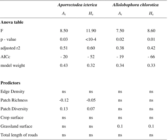
null alleles at some loci (Supplementary data Tables S1 and S2). However, amplification 291
failures observed at loci that did not present heterozygote deficit, highlighted that the lack of 292
amplification may be due to causes other than null alleles such as degraded DNA. 293
Genetic variation within populations
294
Higher values of genetic diversity were obtained for A. chlorotica than for A. icterica 295
(Table 1). For example, standardized allelic richness (Ar) ranged from 6.30 to 9.28 and from 296
1.73 to 3.69 in A. chlorotica and A. icterica, respectively. A significant heterozygosity excess 297
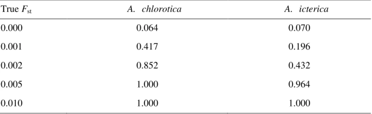
(Wilcoxon test, P<0.05) indicating a recent bottleneck was detected in 1 A. chlorotica and 5 298
A. icterica populations (Table 1). Significant Fis was observed in almost all populations 299
except in PB and I36 for A. chlorotica and in I03, I10 and I31 for A. icterica (Table 1). 300
301
Relationship between genetic diversity and local landscape structure
302
Landscape features in buffers were correlated to genetic diversity in A. icterica and A. 303
chlorotica (Table 3). In A. icterica, the r2 between Ar and He, and landscape features were 304
respectively 0.51 and 0.60 and both were significant (p < 0.05). In this species, patch diversity 305
and patch richness were significantly linked to Ar and He. In A. chlorotica, r2 was 0.38 and 306
0.42, for Ar and He respectively, and both indices were linked to surface in pastures. 307
308
Genetic structure at regional scale
309
The statistical power for both sets of microsatellite loci to detect various levels of true 310
population differentiation (Fst) between populations is presented Table 4. Both sets of markers 311
will detect a true Fst of 0.005 or larger with a probability of 96% or more. The alpha error 312
(corresponding to the probability of obtaining false significances when true Fst = 0) was close 313
to 5% in all cases. 314
All genetic distances matrices (Fst/1-Fst, Fst_COR/1-Fst_COR, Dc and Dc_COR) were 315
significantly correlated with Mantel r value ranging from 0.77 (p = 0.001) to 0.99 (p = 0.001) 316
in A. icterica and from 0.88 (p = 0.001) to 0.99 (p = 0.001) in A. chlorotica (Supplementary 317
data Tables S3, S4 and S5). 318
Fst analysis showed significant genetic structure at the level of the whole study for 319
both species (Fst = 0.059, Fst_COR = 0.055, P<0.001 and Fst = 0.152, Fst_COR = 0.138, P< 0.001 320
for A. chlorotica and A. icterica, respectively). Pairwise Fst estimates ranged from 0.008 to 321
0.116 (Fst_COR ranged from 0.009 to 0.105) and 0.005 to 0.430 (Fst_COR ranged from 0.004 to 322
0.412) for A. chlorotica and A. icterica, respectively (Supplementary data Tables S3 and S4 323
respectively). All exact tests of allelic differentiation were significant (P ≤ 0.005). Analyses 324
using BAPS identified 8 and 12 genetic clusters in A. chlorotica and A. icterica, respectively 325
(P = 0.99 and P = 1 respectively). For A. chlorotica, one cluster was composed of 4 326
populations that were close geographically to one another (PA, PB, I32 and I33), another 327
cluster was composed of the I07, I10, I15 and I18 populations and all other populations 328
corresponded to a different cluster. For A. icterica, 5 clusters were composed of two 329
geographically close populations (PA and PB, I02 and I03, I04 and I32, I07 and I08, I11 and 330
I25) while all other clusters were composed of only one population. Low levels of admixture 331
were observed among the clusters (Supplementary data Fig S1). 332
333
Relationship between genetic differentiation and landscape connectivity
334
Genetic differentiation was linked to landscape connectivity mostly in A. chlorotica 335
(Table 5, Fig 3). In this species resistance distance (CWD) had the most explanatory power, 336
followed by least cost path (LCP) and finally by isolation by distance (IBD). In A. chlorotica, 337
the best scenarios were those in which grasslands were considered to be corridors, whereas 338
crops and roads were considered to be barriers (Table 5). In A. icterica, no significant 339
isolation by distance was found except with the non-corrected Dc distance and the only 340
common point between the several most likely scenarios was that crops were considered as 341
barriers (Table 5). The best congruent models between the two species, taking into account 342
the results from the different genetic indices, were scenarios 9, 10 and 11. The most frequent 343
role of the different landscape element in these scenarios was corridor for grasslands and 344
barrier for crops and roads. Despite significant p-value, it is noteworthy that landscape 345
connectivity was poorly linked to genetic differentiation between A. icterica populations in all 346
cases. 347
Discussion 349
350
Microsatellite markers in earthworms
351
Microsatellites markers have been developed for only a few earthworm species (i.e. 7 352
species so far, review in Torres-Leguizamon et al. 2012; Souleman et al. 2016) and these 353
markers have rarely been used for population genetics studies (but see Velavan et al. 2009; 354
Novo et al. 2010; Dupont et al. 2015). Two different research groups have tried to develop 355
reliable markers for one of the most emblematic European earthworm species, Lumbricus 356
terrestris. Of the ten markers obtained in this species by Velavan et al. (2007), only three 357
were used in a subsequent study (Velavan et al. 2009) suggesting difficulties in genotyping 358
the samples with the other ones. Souleman et al. (2016) couldn’t obtain reliable results with 359
these markers. Thus, they developed eight new markers for which they obtained a low 360
amplification success and a significant heterozygote deficit, suggesting null alleles. In our 361
study, null alleles were suspected at seven out of eight loci in Allobophora chlorotica and at 362
four out of eight loci in Aporrectodea icterica. It is already known that the development of 363
microsatellite molecular markers can be problematic in some taxa (e.g. in molluscs, 364
McInerney et al. 2011 and Lepidoptera, Schmid et al. 2016). It was proposed that such 365
methodological difficulties may have been caused by genomic complexities contained within 366
microsatellite flanking regions. In particular, unstable flanking regions may arise when indels 367
or mutations occur at PCR primer binding sites, thereby causing null alleles (McInerney et al. 368
2011). We therefore believe that microsatellite flanking regions are particularly variable in 369
earthworm species. This could be verified by gathering more genomics data on these taxa. 370
Nevertheless, it seemed that the estimation of genetic divergence was not significantly altered 371
by the presence of null alleles in the dataset. Indeed, similar results were obtained with all 372
indices of genetic divergence (Fst, Fst_COR, Dc, Dc_COR), and correction for the presence of null 373
alleles did not change the results. 374
375
Landscape structure and population genetic diversity
376
Agriculture and urbanization result in habitat loss and fragmentation that variously 377
impact many animal groups. Anthropogenic landscape fragmentation results in reduced size 378
and increased isolation of habitat patches. Fragmented populations are thus expected to 379
experience increased genetic drift and reduced gene flow, which result in the erosion of 380
genetic diversity and the increase of genetic differentiation among local populations 381
(Keyghobadi 2007). Moreover, small populations isolated by surrounding inhospitable 382
landscapes are more vulnerable to demographic variability, environmental stochasticity and 383
genetic processes including inbreeding depression, the random fixation of deleterious alleles 384
and the loss of adaptive potential (Frankham 1995). 385
In this study, we tested how landscape structure in a man-made environment impacted 386
genetic diversity of earthworm populations by characterizing landscape at the buffer scale. A 387
significant relationship was observed between genetic diversity indices (He and Ar) and two 388
features of the immediately surrounding landscape (i.e. patch diversity and patch richness, 389
Table 3) in A. icterica while in A. chlorotica genetic diversity indices were positively linked 390
to surface in pasture. We thus confirmed that geographic isolation of A. icterica populations 391
due to natural and artificial barriers to gene flow probably accentuate the loss of genetic 392
variability through genetic drift, such as already suggested in a previous population genetic 393
study of this species (Torres-Leguizamon et al. 2014). Interestingly, one quarter of the A. 394
icterica populations seemed recently founded, such as revealed by the heterozygosity excess 395
in these populations. Overall, these results suggest that demographic changes occur more 396
frequently in A. icterica than in A. chlorotica and that these demographic changes can be 397
explained by the local landscape structure. 398
399
Genetic differentiation between populations
400
A local decline of effective population size may be explained by the disruption of 401
historical patterns of gene flow in a fragmented habitat (Keyghobadi 2007). Analyses of 402
spatial patterns of genetic structure showed the presence of a strong genetic differentiation in 403
both species, with a low degree of genetic admixture and high Fst values. Fst values were 404
higher for A. icterica, highlighting that these populations are more genetically isolated than 405
the ones of A. chlorotica. This was not expected because A. icterica has a higher potential for 406
active dispersal. Caro et al. (2013) indeed demonstrated in a mesocosm study that A. icterica 407
had a higher dispersal rate than two other endogeic species, namely A. chlorotica and 408
Aporrectodea caliginosa. Moreover, in a recent population genetic study at very fine scale, 409
Dupont et al. (2015) showed a low signal of genetic structure within two A. icterica 410
populations sampled in two plots of less than 1 ha separated by ~ 500m while A. chlorotica 411
populations showed spatial neighbourhood structure in the same sites. This difference was 412
interpreted as a higher dispersal capacity of A. icterica. In the light of the results at very fine 413
scale (Dupont et al. 2015) and at landscape scale (this study), we can assume that A. 414
chlorotica essentially disperse through passive mechanisms over larger distance while passive 415
dispersal might be more restricted for A. icterica. A. chlorotica is a small bodied species and 416
lives near the soil surface in the upper 60 mm soil layer (Sims & Gerard 1999), two features 417
probably facilitating dispersal via various vectors (e.g. zoochory, wind, water and soil transfer 418
via human activities) while A. icterica is found deeper in the soil and is bigger. 419
Landscape connectivity at regional scale
421
The landscape connectivity analysis revealed that genetic structure was linked to 422
landscape connectivity in A. chlorotica, with resistance distance (cwd) having the most 423
explanatory power. Thus, landscape features better explain genetic structure than Euclidian 424
distances in this species. We specifically tested the hypothesis that linear features such as 425
roads may function as dispersal corridors (see for instance Tyser & Worley 1992; Cameron & 426
Bayne 2009) for these species. It has indeed been shown that European earthworms that are 427
invasive in Canada and the northern USA were introduced and spread along road networks 428
(review in Cameron & Bayne 2009). It was however not clear whether the spread of 429
earthworms along roads is more likely to occur via initial transport of earthworms or their 430
cocoons in soil or gravel during road construction or via transport by vehicles after the road 431
has been built (Cameron & Bayne 2009). In addition, roads and sidewalks could also function 432
as dispersal corridors when earthworms crawl out of the soil and disperse at night after heavy 433
rain, as is often observed in some species (e.g. Chuang & Chen 2008). Our results rather 434
suggested that roads constitute obstacles for earthworm dispersal. Using MLPE, we indeed 435
showed that the majority of the most likely landscape connectivity scenarios considered roads 436
as barriers (Table 5). 437
The second hypothesis tested was that grasslands represent a suitable habitat that 438
could be easily crossed by endogeic species and thus represent dispersal corridors, while soil 439
under crops has a detrimental effect on earthworms. These expectations were confirmed by 440
the MLPE analysis, the most likely landscape connectivity scenarios generally considered 441
grasslands as corridors and crops as barriers. 442
Thus, this study suggests that landscape configuration influences gene flow in 443
earthworms. However, no distinct dispersal scenario could be clearly identified, which 444
suggests that passive dispersal due to human activities has also probably played a significant 445
role in shaping genetic structure in both species. 446
447
Conclusion 448
Simultaneously investigating two ecologically similar species highlighted several 449
common features in the response of each species to the landscape. We showed that functional 450
connectivity was impacted by landscape features and that a favourable habitat could act as a 451
corridor for the dispersal of earthworms. We thus confirmed that the aboveground landscape 452
play a part in dispersal and gene flow of below-ground organisms. However, we also 453
observed some differences between species which could be linked to the dispersal and life 454
history attributes of each species. Indeed, population genetic diversity was significantly 455
influenced by the local landscape structure in both species, but only the genetic differentiation 456
of A. chlorotica populations was related to functional connectivity. This result highlights that 457
the exact effect of each habitat type on genetic variation over space and time and of 458
agricultural practices on earthworm dispersal should be studied using specific sampling 459
strategies. 460
461
Acknowledgements 463
This work was funded by the French National Research Agency (ANR) as a part of the 464
project EDISP no. ANR-08-JCJC-0023 leaded by Jerome Mathieu. We thank all the 465
participants to the EDISP project for their participation to field sampling. We also thank 466
Roger Hijmans and Jacob van Etten for their advice on GIS analysis in R, Marteen J. Van 467
Strien for the R script to perform MLPE and Naoise Nunan for English language editing. 468
469
470
References 472
Adriaensen F, Chardon JP, De Blust G, et al. (2003) The application of "least-cost" modelling as a 473
functional landscape model. Landscape and Urban Planning, 64, 233-247. 474
Belkhir K, Borsa P, Goudet J, Chikhi L Bonhomme F (2004) GENETIX 4.05, logiciel sous Windows pour 475
la génétique des populations. Laboratoire Génome, Population, Interactions, CNRS UMR 476
5000, Université Montpellier II, Montpellier (France). 477
Benjamini Y Hochberg Y (1995) Controlling the False Discovery Rate - a Practical and Powerful 478
Approach to Multiple Testing. Journal of the Royal Statistical Society Series B-Methodological, 479
57, 289-300.
480
Bertrand M, Barot S, Blouin M, et al. (2015) Earthworm services for cropping systems. A review. 481
Agronomy for Sustainable Development, 35, 553-567.
482
Blouin M, Hodson ME, Delgado EA, et al. (2013) A review of earthworm impact on soil function and 483
ecosystem services. European Journal of Soil Science, 64, 161-182. 484
Bouché MB (1972) Lombriciens de France. Ecologie et systématique INRA, Paris. 485
Bouché MB (1977) Stratégies lombriciennes. In: Soil organisms as components of ecosystems. (eds. 486
Lohm, U., Persson, T.), pp. 122-132. Ecological Bulletin, Stockholm. 487
Cameron EK Bayne EM (2009) Road age and its importance in earthworm invasion of northern boreal 488
forests. Journal of Applied Ecology, 46, 28-36. 489
Caro G, Abourachid A, Decaëns T, Buono L Mathieu J (2012) Is earthworms' dispersal facilitated by 490
the ecosystem engineering activities of conspecifics? Biology and Fertility of Soils, 48, 961-491
965. 492
Caro G, Decaëns T, Lecarpentier C Mathieu J (2013) Are dispersal behaviours of earthworms related 493
to their functional group? Soil Biology & Biochemistry, 58, 181-187. 494
Cavalli-Sforza LL Edwards AWF (1967) Phylogenetic analysis. Models and estimation procedures. 495
American Journal of Human Genetics, 19, 233-257.
496
Chapuis MP Estoup A (2007) Microsatellite null alleles and estimation of population differentiation. 497
Molecular Biology and Evolution, 24, 621-631.
498
Chuang SC Chen JH (2008) Role of diurnal rhythm of oxygen consumption in emergence from soil at 499
night after heavy rain by earthworms. Invertebrate Biology, 127, 80-86. 500
Clark M, Tanguy A, Jollivet D, et al. (2010) Populations and Pathways: Genomic approaches to 501
understanding population structure and environmental adaptation. In: Introduction to 502
marine genomics (eds. Cock, M.J., Tessmar-Raible, K., Boyen, C., Viard, F.), pp. 73-118. 503
Springer. 504
Corander J Marttinen P (2006) Bayesian identification of admixture events using multilocus 505
molecular markers. Molecular Ecology, 15, 2833-2843. 506
Corander J, Sirén J Arjas E (2008) Bayesian spatial modelling of genetic population structure. 507
Computational Statistics, 23, 111-129.
508
Cornuet J-M Luikart G (1996) Description and power analysis of two tests for detecting recent 509
population bottlenecks from allele frequency data. Genetics, 144, 2001-2014. 510
Costa D, Timmermans MJTN, Sousa JP, et al. (2013) Genetic structure of soil invertebrate 511
populations: Collembolans, earthworms and isopods. Applied Soil Ecology, 68, 61-66. 512
Decaens T, Margerie P, Aubert M, Hedde M Bureau F (2008) Assembly rules within earthworm 513
communities in North-Western France - A regional analysis. Applied Soil Ecology, 39, 321-514
335. 515
Dormann CF, Elith J, Bacher S, et al. (2013) Collinearity: a review of methods to deal with it and a 516
simulation study evaluating their performance. Ecography, 36, 27-46. 517
Dupont L, Grésille Y, Richard B, Decaëns T Mathieu J (2015) Fine-scale spatial genetic structure and 518
dispersal constraints in two earthworm species. Biological Journal of the Linnean Society, 519
114, 335-347.
520
Dupont L, Lazrek F, Porco D, et al. (2011) New insight into the genetic structure of the Allolobophora 521
chlorotica aggregate in Europe using microsatellite and mitochondrial data. Pedobiologia, 54,
522
217-224. 523
Eijsackers H (2011) Earthworms as colonizers of natural and cultivated soil environments. Applied Soil 524
Ecology, 50, 1-13.
525
Frankham R (1995) Conservation genetics. Annual Review of Genetics, 29, 305-327. 526
Goudet J (2000) FSTAT, a program to estimate and test gene diversities and fixation indices. Available 527
from http://www.unil.ch/izea/softwares/fstat.html. 528
Hall LA Beissinger SR (2014) A practical toolbox for design and analysis of landscape genetics studies. 529
Landscape Ecology, 29, 1487-1504.
530
Holderegger R Wagner HH (2008) Landscape genetics. Bioscience, 58, 199-207. 531
Jouquet P, Dauber J, Lagerlof J, Lavelle P Lepage M (2006) Soil invertebrates as ecosystem engineers: 532
Intended and accidental effects on soil and feedback loops. Applied Soil Ecology, 32, 153-164. 533
Keyghobadi N (2007) The genetic implications of habitat fragmentation for animals. Canadian Journal 534
of Zoology, 85, 1049-1064.
535
Lavelle P, Bignell D, Lepage M, et al. (1997) Soil function in a changing world: the role of invertebrate 536
ecosystem engineers. European Journal of Soil Biology, 33, 159-193. 537
Lavelle P, Decaens T, Aubert M, et al. (2006) Soil invertebrates and ecosystem services. European 538
Journal of Soil Biology, 42, S3-S15.
539
Manel S Holderegger R (2013) Ten years of landscape genetics. Trends in Ecology & Evolution, 28, 540
614-621. 541
Manel S, Schwartz MK, Luikart G Taberlet P (2003) Landscape genetics: combining landscape ecology 542
and population genetics. Trends in Ecology & Evolution, 18, 189-197. 543
Mantel N (1967) The detection of disease clustering and a generalized regression approach. Cancer 544
Research, 27, 209-220.
545
Mathieu J, Barot S, Blouin M, et al. (2010) Habitat quality, conspecific density, and habitat pre-use 546
affect the dispersal behaviour of two earthworm species, Aporrectodea icterica and 547
Dendrobaena veneta, in a mesocosm experiment. Soil Biology and Biochemistry, 42, 203-209.
548
Matthysen E (2012) Multicausality of dispersal : a review. In: Dispersal Ecology and Evolution (eds. 549
Clobert, J., Baguette, M., Benton, T.G., Bullock, J.M.), pp. 3-18. Oxford University Press, 550
Oxford. 551
McGarigal K, Cushman SA Ene E (2012) FRAGSTATS v4: Spatial Pattern Analysis Program for 552
Categorical and Continuous Maps., p. Available at the following web site: 553
http://www.umass.edu/landeco/research/fragstats/fragstats.html. produced by the authors 554
University of Massachusetts, Amherst. 555
McInerney CE, Allcock AL, Johnson MP, Bailie DA Prodohl PA (2011) Comparative genomic analysis 556
reveals species-dependent complexities that explain difficulties with microsatellite marker 557
development in molluscs. Heredity, 106, 78-87. 558
McRae BH (2006) Isolation by resistance. Evolution, 60, 1551-1561. 559
McRae BH Nürnberger B (2006) Isolation by resistance. Evolution, 60, 1551-1561. 560
Montgomery DC Peck EA (1992) Introduction to Linear Regression Analysis. Wiley, New York. 561
Novo M, Almodovar A, Fernandez R, Gutierrez M Cosin DJD (2010) Mate choice of an endogeic 562
earthworm revealed by microsatellite markers. Pedobiologia, 53, 375-379. 563
Palm J, van Schaik NLMB Schroeder B (2013) Modelling distribution patterns of anecic, epigeic and 564
endogeic earthworms at catchment-scale in agro-ecosystems. Pedobiologia, 56, 23-31. 565
Piry S, Luikart G Cornuet JM (1999) BOTTLENECK: A Computer Program for Detecting Recent 566
Reductions in the Effective Population Size Using Allele Frequency Data. Journal of Heredity, 567
90, 502-503.
568
Pompanon F, Bonin A, Bellemain E Taberlet P (2005) Genotyping errors: Causes, consequences and 569
solutions. Nature Reviews Genetics, 6, 847-859. 570
R Development Core Team (2012) R : A language and environment for statistical computing. In: R 571
Foundation for Statistical Computing, Vienna, Austria.
572
Richard B, Legras M, Margerie P, et al. (2012) Spatial organization of earthworm assemblages in 573
pastures of northwestern France. European Journal of Soil Biology, 53, 62-69. 574
Rousset F (2008) GENEPOP ' 007: a complete re-implementation of the GENEPOP software for 575
Windows and Linux. Molecular Ecology Resources, 8, 103-106. 576
Ryman N Palm S (2006) POWSIM: a computer program for assessing statistical power when testing 577
for genetic differentiation. Molecular Ecology Notes, 6, 600-602. 578
Schmid M, Csencsics D Gugerli F (2016) Repetitive flanking sequences challenge microsatellite 579
marker development: a case study in the lepidopteran Melanargia galathea. Molecular 580
Ecology Resources, 16, 1499-1507.
581
Sims RW Gerard BM (1999) Synopsis of the British Fauna (31)- earthworms, pp. 1-169. The Linnean 582
Society of London and the Estuarine and Brackish-water Sciences association, London. 583
Souleman D, Grumiaux F, Frerot H, Vandenbulcke F Pauwels M (2016) Isolation and characterization 584
of eight polymorphic microsatellites markers for the earthworm Lumbricus terrestris. 585
European Journal of Soil Biology, 74, 76-80.
586
Spear SF, Balkenhol N, Fortin MJ, McRae BH Scribner K (2010) Use of resistance surfaces for 587
landscape genetic studies: considerations for parameterization and analysis. Molecular 588
Ecology, 19, 3576-3591.
589
Storfer A, Murphy MA, Evans JS, et al. (2007) Putting the 'landscape' in landscape genetics. Heredity, 590
98, 128-142.
591
Storfer A, Murphy MA, Spear SF, Holderegger R Waits LP (2010) Landscape genetics: where are we 592
now? Molecular Ecology, 19, 3496-3514. 593
Sullivan TJ, Dreyer AP Peterson JW (2009) Genetic variation in a subterranean arthropod (Folsomia 594
candida) as a method to identify low-permeability barriers in an aquifer. Pedobiologia, 53, 595
99-105. 596
Taylor P, Fahrig L With KA (2006) Landscape connectivity: back to the basics. In: Connectivity 597
Conservation (eds. Crooks, K., Sanjayan, M.A.), pp. 29–43. Cambridge University Press, 598
Cambridge. 599
Taylor PD, Fahrig L, Henein K Merriam G (1993) Connectivity Is a Vital Element of Landscape 600
Structure. Oikos, 68, 571-573. 601
Torres-Leguizamon M, Mathieu J, Decaëns T Dupont L (2014) Genetic structure of earthworm 602
populations at a regional scale: inferences from mitochondrial and microsatellite molecular 603
markers in Aporrectodea icterica (Savigny 1826). Plos One, 9, e101597. 604
Torres-Leguizamon M, Mathieu J, Livet A Dupont L (2012) Isolation of polymorphic microsatellite 605
markers in Aporrectodea icterica (Savigny 1826). Soil Biology & Biochemistry, 51, 16-19. 606
Tyser RW Worley CA (1992) Alien flora in grasslands adjacent to road and trail corridors in glacier 607
national-park, Montana (USA) Conservation Biology, 6, 253-262. 608
Van Oosterhout C, Hutchinson WF, Wills DPM Shipley P (2004) MICRO-CHECKER: software for 609
identifying and correcting genotyping errors in microsatellite data. Molecular Ecology Notes, 610
4, 535-538.
611
Van Strien MJ, Keller D Holderegger R (2012) A new analytical approach to landscape genetic 612
modelling: least-cost transect analysis and linear mixed models. Molecular Ecology, 21, 4010-613
4023. 614
Vanbergen AJ, Watt AD, Mitchell R, et al. (2007) Scale-specific correlations between habitat 615
heterogeneity and soil fauna diversity along a landscape structure gradient. Oecologia, 153, 616
713-725. 617
Velavan TP, Schulenburg H Michiels N (2007) Development and characterization of novel 618
microsatellite markers for the common earthworm (Lumbricus terrestris L). Mol. Ecol. Notes, 619
7, 1060-1062.
620
Velavan TP, Weller S, Schulenburg H Michiels NK (2009) High genetic diversity and heterogeneous 621
parasite load in the earthworm Lumbricus terrestris on a German meadow. Soil Biology & 622
Biochemistry, 41, 1591-1595.
623
Weir BS Cockerham CC (1984) Estimating F-statistics for the analysis of population structure. 624
Evolution, 38, 1358-1370.
625
Zeller K, McGarigal K Whiteley A (2012) Estimating landscape resistance to movement: a review. 626
Landscape Ecology, 27, 777-797.
627
Zuur AF, Ieno EN Elphick CS (2010) A protocol for data exploration to avoid common statistical 628
problems. Methods in Ecology and Evolution, 1, 3-14. 629
630 631
632
Data Accessibility 634
The data sets with the microsatellite genotypes of A. chlorotica and A. icterica are available 635
from the Dryad Digital Repository: http://dx.doi.org/10.5061/dryad.sc6bb. 636
637
Author Contributions 639
J.M initiated the project. L.D. and J.M. designed the study. L.D. drafted the manuscript. L.D., 640
M.T.L., P. R.-C. and J.M. collected the data. L.D and P. R.-C. performed molecular analyses. 641
J.M. built the GIS database and conducted the landscape genetic analyses (Buffer and 642
connectivity). L.D. and J.M. performed statistical analyses and wrote the manuscript. 643
644
Figure legends 646
647
Figure 1 648
Illustration of the different landscape genetic approaches used in this work. a) Local genetic 649
structure is compared to local landscape features within a buffer around each population; b) 650
genetic difference is linked to geographical distance between populations (IBD); c) genetic 651
difference is linked to the functional distance between populations, calculated as the least cost 652
path between populations (LCP), based on a resistance map; d) genetic difference is linked to 653
the functional distance between populations, calculated as the sum of the cost weighted paths 654
between populations (cwd), based on a resistance map. 655
656
Figure 2 657
Geographical distribution of earthworm sampling sites near Yvetot in Normandy (France). 658
“No species” means that neither A. icterica nor A. chlorotica were found. 659
660
Figure 3 661
Best correlation found between genetic distance (Dc distance) and resistance distance scenario 662
(cwd) for A. chlorotica (A) and A. icterica (B). 663
664
665
666
Table 1. Geographical location*, sample size (N), genetic diversity (Ar: standardized allelic richness; He: expected heterozygosity), fixation index
Fis (significant values are in bold) and Wilcoxon test P value for heterozygote excess compared to expectations at mutation-drift equilibrium
(pwil) for each study plot and each species. *Latitude/longitude range in Lambert II étendu.
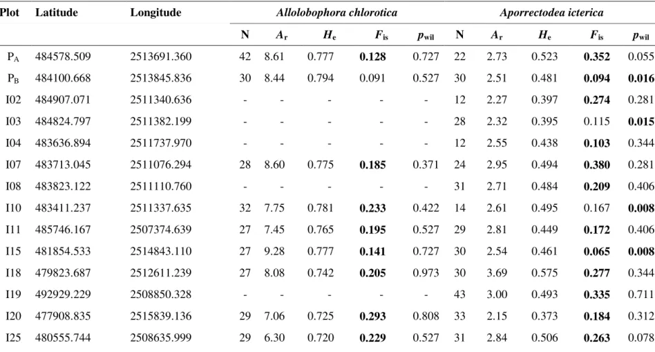
Plot Latitude Longitude Allolobophora chlorotica Aporrectodea icterica
N Ar He Fis pwil N Ar He Fis pwil PA 484578.509 2513691.360 42 8.61 0.777 0.128 0.727 22 2.73 0.523 0.352 0.055 PB 484100.668 2513845.836 30 8.44 0.794 0.091 0.527 30 2.51 0.481 0.094 0.016 I02 484907.071 2511340.636 - - - - - 12 2.27 0.397 0.274 0.281 I03 484824.797 2511382.199 - - - - - 28 2.32 0.395 0.115 0.015 I04 483636.894 2511737.970 - - - - - 12 2.55 0.438 0.103 0.344 I07 483713.045 2511076.294 28 8.60 0.775 0.185 0.371 24 2.95 0.494 0.380 0.281 I08 483823.122 2511110.760 - - - - - 31 2.71 0.484 0.209 0.406 I10 483411.237 2511337.635 32 7.75 0.781 0.233 0.422 14 2.61 0.495 0.167 0.008 I11 485746.167 2507374.639 27 7.45 0.765 0.195 0.527 29 2.81 0.449 0.172 0.406 I15 481854.533 2514843.110 27 9.28 0.777 0.141 0.727 30 2.54 0.461 0.065 0.008 I18 479823.687 2512611.239 27 8.08 0.742 0.205 0.973 30 3.69 0.575 0.277 0.344 I19 492929.229 2508850.328 - - - - - 43 3.00 0.493 0.335 0.711 I20 477908.835 2515839.136 29 7.06 0.725 0.293 0.808 33 2.15 0.373 0.184 0.312 I25 480555.744 2508635.999 29 6.30 0.720 0.229 0.527 31 2.84 0.506 0.263 0.078
I27 489902.819 2513148.683 30 8.81 0.788 0.156 0.770 34 2.62 0.485 0.317 0.023 I31 482053.828 2513328.538 - - - - - 27 1.73 0.226 0.115 0.594 I32 483297.736 2513724.785 29 8.16 0.786 0.179 0.273 30 2.70 0.422 0.305 0.656 I33 481742.786 2511459.498 32 8.61 0.761 0.182 0.902 29 2.52 0.454 0.179 0.148 I34 482430.931 2510886.051 32 7.95 0.747 0.237 0.875 30 2.33 0.366 0.403 0.078 I36 487833.362 2509076.597 46 6.67 0.777 0.067 0.010 - - -
Table 2 Role and cost of landscape elements in the different landscape scenarios tested in this study. The cost of grasslands, crops and roads changed among scenarios. Costs of permanent water bodies (20), temporary water bodies (1), deciduous forest (20), coniferous forest (20), hedges (20) and urban area (50) were fixed in all scenarios.
Role of elements Cost of elements
Scenario Grasslands Crops Roads Grasslands Crops Roads
1 Barrier Barrier Barrier 50 50 50
2 Barrier Barrier Neutral 50 50 20
3 Barrier Barrier Corridor 50 50 1
4 Barrier Corridor Barrier 50 1 50
5 Barrier Corridor Neutral 50 1 20
6 Barrier Corridor Corridor 50 1 1
7 Barrier Neutral Barrier 50 20 50
8 Barrier Neutral Neutral 50 20 20
9 Barrier Neutral Corridor 50 20 1
10 Corridor Barrier Barrier 1 50 50
11 Corridor Barrier Neutral 1 50 20
12 Corridor Barrier Corridor 1 50 1
13 Corridor Corridor Barrier 1 1 50
14 Corridor Corridor Neutral 1 1 20
15 Corridor Corridor Corridor 1 1 1
16 Corridor Neutral Barrier 1 20 50
17 Corridor Neutral Neutral 1 20 20
18 Corridor Neutral Corridor 1 20 1
19 Neutral Barrier Barrier 20 50 50
20 Neutral Barrier Neutral 20 50 20
21 Neutral Barrier Corridor 20 50 1
22 Neutral Corridor Barrier 20 1 50
23 Neutral Corridor Neutral 20 1 20
24 Neutral Corridor Corridor 20 1 1
25 Neutral Neutral Barrier 20 20 50
26 Neutral Neutral Neutral 20 20 20
Table 3 Summary of the best multiple regression between landscape features (predictors) and genetic diversity (Ar: Allele Richness, He: expected heterozygosity) of the populations of the two earthworm species A. icterica and A. chlorotica in the region of Yvetot, Normandy, France, based on AICc weight. A patch represents an element in the landscape and the buffer radius was 500m. Predictors are: Edge Density (length of patch edge/surface of the buffer), Patch Richness (number of different types of patches in the buffer), Patch Diversity (Shannon Diversity of the different Land Use types), Crop surface, Grassland surface and Total length of roads.
Aporrectodea icterica Allolobophora chlorotica
Ar He Ar He Anova table F 8.50 11.90 7.50 8.60 p - value 0.03 <10-4 0.02 0.01 adjusted r2 0.51 0.60 0.38 0.42 AICc - 20 - 52 - 19 - 66 model weight 0.43 0.32 0.34 0.33 Predictors Edge Density ns ns ns ns Patch Richness -0.12 -0.05 ns ns Patch Diversity 0.13 0.07 ns ns Crop surface ns ns ns ns Grassland surface ns ns 0.1 0.1
Table 4 Statistical power for detecting various true levels of population differentiation (Fst) by means of Fisher’s exact test when using both sets of microsatellite loci, allele frequencies, and sample sizes. The power is expressed as the proportion of simulations that provide statistical significance at the 0.05 level.
True Fst A. chlorotica A. icterica
0.000 0.064 0.070
0.001 0.417 0.196
0.002 0.852 0.432
0.005 1.000 0.964
Table 5 Summary of the link between landscape connectivity and genetic structure (MLPE), comparing A. Euclidian distance and genetic
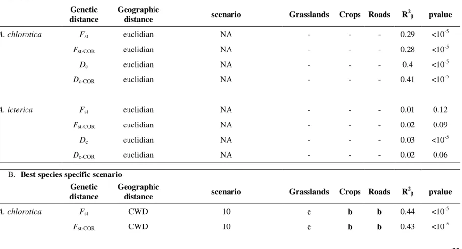
differentiation (pairwise Fst , pairwise Fst estimates corrected for null alleles, Dc genetic distance and Dc genetic distance corrected for null
alleles) between populations (Isolation by distance, IBD).and B. cost weighted distances (cwd) and genetic differentiation between populations. The most likely landscape connectivity scenarios are indicated. The roles of the landscape elements in the most likely
scenarios are specified (b = barrier, c = corridor and n = neutral); when applicable the most frequent role is in bold. In C. the best congruent scenarios are presented. The R2β statistic described by Van Strien et al (2012) is presented. NA = Not Applicable
A. IBD
Genetic distance
Geographic
distance scenario Grasslands Crops Roads R
2 β pvalue A. chlorotica Fst euclidian NA - - - 0.29 <10-5 Fst-COR euclidian NA - - - 0.28 <10-5 Dc euclidian NA - - - 0.4 <10-5 Dc-COR euclidian NA - - - 0.41 <10-5 A. icterica Fst euclidian NA - - - 0.01 0.12 Fst-COR euclidian NA - - - 0.02 0.09 Dc euclidian NA - - - 0.03 <10-5 Dc-COR euclidian NA - - - 0.02 0.06
B. Best species specific scenario
Genetic distance
Geographic
distance scenario Grasslands Crops Roads R
2
β pvalue
A. chlorotica Fst CWD 10 c b b 0.44 <10-5
Dc CWD 8, 9, 10 b, c b, n b, n, c 0.54 <10-5 Dc-COR CWD 8, 9, 14 b, c n, c n, c 0.54 <10-5 A. icterica Fst CWD 1, 2, 3, 11, 12, 21 b, n, c b, c b, n, c 0.04 <10 -4 Fst-COR CWD 1, 2, 3, 11, 12, 21 b, n, c b, c b, n, c 0.05 <10-4 Dc CWD 1, 2, 3, 11, 12, 21 b, n, c b, c b, n, c 0.08 <10-5 Dc-COR CWD 1, 11, 12, 21, 25, 26, 27 b, n, c b, n b, n, c 0.06 <10-5
C. Best congruent scenario
Genetic distance
Geographic
distance scenario Grasslands Crops Roads R
2 β pvalue A.chlorotica Fst CWD 10 c b b 0.44 <10-5 Fst-COR CWD 10 c b b 0.43 <10-5 Dc CWD 9, 10 b, c n, b b, c 0.54 <10-5 Dc-COR CWD 9, 10, 11 b, c n, b b, n, c 0.54 <10-5 A.icterica Fst CWD 10 c b b 0.04 <10-4 Fst-COR CWD 10 c b b 0.04 <10-4 Dc CWD 9, 10 b, c n, b b, c 0.07 <10-5 Dc-COR CWD 9, 10, 11 b, c n, b b, n, c 0.06 <10-4