HAL Id: hal-00317302
https://hal.archives-ouvertes.fr/hal-00317302
Submitted on 2 Apr 2004
HAL is a multi-disciplinary open access
archive for the deposit and dissemination of
sci-entific research documents, whether they are
pub-lished or not. The documents may come from
teaching and research institutions in France or
abroad, or from public or private research centers.
L’archive ouverte pluridisciplinaire HAL, est
destinée au dépôt et à la diffusion de documents
scientifiques de niveau recherche, publiés ou non,
émanant des établissements d’enseignement et de
recherche français ou étrangers, des laboratoires
publics ou privés.
and electric fields as a function of altitude using
Polar/EFI data
P. Janhunen, A. Olsson, H. Laakso
To cite this version:
P. Janhunen, A. Olsson, H. Laakso. The occurrence frequency of auroral potential structures and
elec-tric fields as a function of altitude using Polar/EFI data. Annales Geophysicae, European Geosciences
Union, 2004, 22 (4), pp.1233-1250. �hal-00317302�
SRef-ID: 1432-0576/ag/2004-22-1233 © European Geosciences Union 2004
Annales
Geophysicae
The occurrence frequency of auroral potential structures and
electric fields as a function of altitude using Polar/EFI data
P. Janhunen1, A. Olsson2, and H. Laakso3
1Finnish Meteorological Institute, Geophysical Research, Helsinki, Finland
2Swedish Institute of Space Physics, Uppsala Division, Uppsala, Sweden
3ESTEC, Space Science Department, Noordwijk, The Netherlands
Received: 15 January 2003 – Revised: 28 August 2003 – Accepted: 4 September 2003 – Published: 2 April 2004
Abstract. The aim of the paper is to study how auroral
potential structures close at high altitude. We analyse all electric field data collected by Polar on auroral field lines in 1996–2001 by integrating the electric field along the space-craft orbit to obtain the plasma potential, from which we identify potential minima by an automatic method. From these we estimate the associated effective mapped-down
electric field Ei, defined as the depth of the potential
mini-mum divided by its half-width in the ionosphere. Notice that although we use the ionosphere as a reference altitude, the
field Ei does not actually exist in the ionosphere but is just
a convenient computational quantity. We obtain the
statisti-cal distribution of Eias a function of altitude, magnetic local
time (MLT), Kp index and the footpoint solar illumination
condition. Surprisingly, we find two classes of electric field structures. The first class consists of the low-altitude poten-tial structures that are presumably associated with inverted-V regions and discrete auroral arcs and their set of associ-ated phenomena. We show that the first class exists only
below ∼3 RE radial distance, and it occurs in all nightside
MLT sectors (RE=Earth radius). The second class exists
only above radial distance R=4 RE and almost only in the
midnight MLT sector, with a preference for high Kp values.
Interestingly, in the middle altitudes (R=3−4 RE) the
num-ber of potential minima is small, suggesting that the low and high altitude classes are not simple field-aligned extensions of each other. This is also underlined by the fact that statisti-cally the high altitude structures seem to be substorm-related, while the low altitude structures seem to correspond to sta-ble auroral arcs. The new finding of the existence of the two classes is important for theories of auroral acceleration, since it supports a closed potential structure model for stable arcs, while during substorms, different superposed processes take place that are associated with the disconnected high-altitude electric field structures.
Key words. Magnetospheric physics (electric fields;
auro-ral phenomena) – Space plasma physics (electrostatic struc-tures)
Correspondence to: P. Janhunen
(pekka.janhunen@fmi.fi)
1 Introduction
Strong, up to several hundred millivolts per meter, perpendic-ular electric fields exist at around 5000–13 000 km altitude in conjunction with optical auroral arcs and inverted-V electron precipitation (Mozer et al., 1977). Closer examination of the perpendicular electric fields reveals that they often form a convergent electric field signature (electric fields pointing to-ward each other in close spatial separation). That the pairs of convergent electric fields are typically not caused by tem-poral variations can be inferred from the fact that upgoing ion beam energies match with the potential V integrated from the boundary of the structure along the satellite orbit, V =−R ds×E (McFadden et al., 1998). The potentials V ob-tained in this way also agree with typical inverted-V elec-tron energies measured at lower altitudes. Thus, it seems that there exists a negative potential structure for each inverted-V event. From the fact that the occurrence frequency of strong convergent electric fields goes down with decreasing altitude, it was concluded that the potential contours must close above the ionosphere, thus forming an upward parallel electric field (Torbert and Mozer, 1978; Mozer et al., 1980; Bennett et al., 1983). This also supports the view that the U-shaped po-tential model is responsible for generating inverted-V type electron energy spectra (Carlqvist and Bostr¨om, 1970).
The widths of the potential structures should match the typical widths of inverted-V regions and optical auroral arcs. The widths of inverted-V regions and optical arcs match each other when compared with compatible criteria (Stenbaek-Nielsen et al., 1998; Hallinan et al., 2001). In this paper we consider widths in the range 500 m–60 km. This width range should contain almost all auroral arcs, apart from the most narrow ones (Maggs and Davis, 1968; Borovsky, 1993; Knudsen et al., 2001). Knudsen et al. (2001) used the term “mesoscale arc” to refer to what we call “auroral arc” in this paper.
Since there is a lot of support for the U-shaped po-tential model from low-altitude observations (altitude be-low 13 000 km), a natural question arises in what way the U-shaped potential contours continue at higher altitudes. It is topologically necessary that all potential contours close
somewhere within the flux tube, either below the equatorial plane or in the opposite hemisphere. In this paper, by
“low-altitude” we refer to radial distances below 3 REwhich
corre-sponds to altitude 13 000 km. Surprisingly, no clear evidence of significant convergent electric field signatures was found above about 20 000 km altitude in a statistical study using 78 events for which simultaneous ground magnetometer data were available to rule out substorm cases (Janhunen et al., 1999). Stable arcs are so common phenomena that among 78 events there should be some, thus the indirect implication was that above stable arcs, no clear evidence of significant convergent fields was found.
In this paper we revisit the potential structure closure ques-tion in a more thorough and quantitative way by using a much larger data set and complete altitude coverage. Our expanded study is now made possible by the fact that the orbit of Polar has evolved in such a way that no altitude gaps remain within 5000–30 000 km. We study potential structures of various depths as a function of altitude, without, however, forgetting
magnetic local time (MLT), solar illumination and Kp
in-dex dependence. In particular, we investigate the so-called
effective electric field Ei, defined as the depth of the
poten-tial minimum divided by the width of the structure in the ionosphere. Notice that although we use the ionosphere as
a reference altitude, the field Ei does not actually exist in
the ionosphere but is just a convenient computational quan-tity. The statistical results can reveal important facts that can be used to constrain various theories that have been put for-ward to self-consistently explain the yet unsolved electron acceleration mechanism whose manifestations are potential structures, inverted-V regions, ion beams, and auroral arcs (Carlqvist and Bostr¨om, 1970; Bryant and Perry, 1995; Jan-hunen and Olsson, 2000). To complement the study of po-tential minimum associated electric fields, in Sect. 5 we will also present results concerning the altitude distribution of all perpendicular electric fields (i.e. not only those that are asso-ciated with potential minima). That substudy is slightly sim-ilar to a statistical study by Lindqvist and Marklund (1990),
who used Viking data up to 14 000 km altitude (3.2 REradial
distance).
We use the following terminology. “Altitude (h)” means distance from Earth’s surface and “radial distance (R)” means distance from the centre of the Earth
(geocen-tric distance). They are connected by R=RE+h, where
RE=6 371.2 km is Earth’s radius. We usually express
alti-tude in kilometres and radial distance in RE. In the figures,
radial distance R is used.
2 Instrumentation
The Polar Electric Field Investigation (EFI) instrument mea-sures the instantaneous electric field in the satellite spin plane continuously with at least 20 samples per second (Harvey et al., 1995). The measurement is made with two pairs of long wire booms, called 1–2 and 3–4. Also, the component which is parallel to the spin axis is measured with a fixed
boom pair (called 5–6), which does not, however, always produce an accurate measurement because of the shortness of the booms. Fortunately, since the spin and orbital planes of the satellite are very nearly equal, the 5–6 component hardly contributes anything to the line integral V of the electric field, V =−R ds×E. Thus, we assumed that the 5–6 component is zero instead of using the measured value in our basic sta-tistical studies. To verify that the results do not depend on this assumption we repeated part of the analysis by using the measured 5–6 component and also, as a third option, the elec-tric field computed from 1–2, 3–4 and the condition E×B=0. We found that the potential minima computed by the three different methods gave very nearly the same result.
During intense cold ion outflow events, a wake effect par-allel to the magnetic field may develop which may cause an offset of ∼5 mV/m in the parallel component if the magnetic field is close to the spin plane, as it is in many of our events. A manual inspection of some of our events showed, however, that this effect does not play a role in our data set. One rea-son is that we only use the component of the electric field which is parallel to the spacecraft velocity vector, which is usually approximately perpendicular in the auroral crossings. We also use the Magnetic Field Experiment (MFE) on board Polar (Russell et al., 1995) to reject events where the satellite moves too much parallel to the magnetic field.
3 Data processing
3.1 Data selection
Only the invariant latitude (ILAT) range 64◦–75◦ is included
in the analysis. As ILAT values we use the dipolar ILAT pa-rameter values found in standard Polar orbital CDF files.
Fur-thermore, radial distances only up to R= 6REare considered
because at higher radial distances the satellite travel times over the auroral zone become inconveniently long. Only complete auroral crossings are included, i.e. ones in which
the ILAT of Polar changes monotonically between 64◦ and
75◦. Likewise, if any part of the auroral crossing as
de-termined from ILAT has the radial distance beyond 6 RE,
the crossing is not included in the database. Eclipse periods where the satellite is in the optical shadow of the Earth are re-moved because the DC electric field double probe measure-ments may not be reliable. Also, periods when the Plasma Source Instrument (PSI) (Moore et al., 1995) is operating are removed.
3.2 How potential minima are found and processed
The data processing starts from the plasma potential as a function of time, i.e. the potential V (t ) integrated along the spacecraft orbit using the spin plane electric field, and has the following steps:
1. The potential V is interpolated to 0.005◦ILAT grid
spacing, which corresponds to about 500 m resolution in the ionosphere. The temporal resolution of 20 samples
per second would enable even somewhat higher ILAT resolution, but the chosen resolution was considered sufficient for this study. Based on Knudsen et al. (2001), a mean width of an auroral arc is 18±9 km so that 500 m resolution is high enough.
2. All local minima are found from the ILAT-interpolated potential, i.e. all data points that have a smaller value than their immediate predecessor and successor. 3. A search is initiated left and right from each local
mini-mum, stopping when the values start to decrease again. This produces a tentative interval for the minimum re-gion.
4. The depth of the minimum is defined to be the differ-ence of values at the minimum and at the point (ei-ther left or right, whichever yields the smaller depth) where points started to decrease again. This means that some potential minima are possibly underestimated, es-pecially when a minimum occurs at an edge of a larger minimum.
5. A region around the minimum is found which satisfies
the condition V ≤Vmin+0.5 Vdepthwhere Vminis the
po-tential value at the local minimum and Vdepth, is the
min-imum depth defined in the previous item. The width of the minimum is then defined to be the ILAT extent of the region. This corresponds to width at the half maximum.
6. Interpolation of the data to a new ILAT grid having half the previous resolution is carried out, and the above steps are repeated. This is done in order to prevent left/right searches from getting stuck with local fluctua-tions, i.e. the data vector is analysed in multiple spatial scales in order to find the minima at any scale. This is repeated recursively to higher coarsening levels until the
ILAT spacing is large (>0.5◦). This is the most
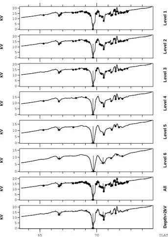
impor-tant point of our analysis. The procedure is illustrated in Fig. 1. The first six panels show the original data (top panel), together with five subsequent smoothed ver-sions. The potential becomes smoother in each panel as compared to the panel above. The minima found at each stage are shown as dots. The widths and depths of the minima are indicated by horizontal and vertical lines, respectively. The figure also contains two other panels which are discussed below after item 8.
7. The parameters (location, width, etc.) of all minima are stored in a file.
8. As a postprocessing step, minima that are too close to each other are replaced by one (the one with the largest depth is selected among equivalent ones). Two min-ima (belonging to the same auroral pass) are considered equivalent, if and only if all the following conditions hold: 0 5 10 15 20 kV Level 1 0 5 10 15 20 kV Level 2 0 5 10 15 20 kV Level 3 0 5 10 15 kV Level 4 0 5 10 15 kV Level 5 0 5 10 15 kV Level 6 0 5 10 15 20 kV All 65 70 ILAT 0 5 10 15 20 kV Depth>2kV
Fig. 1. Illustration of the potential minimum finding algorithm.
Panels 1–6 show the first six coarsening levels. Dots show each located local minimum and its width and depth by horizontal and vertical lines, respectively. Panel 7 shows all potential minima after postprocessing (equivalents removed and replaced by the deepest minimum). Panel 8 is same as panel 7, except showing only poten-tial minima deeper than 2 kV. In the actual analysis the limit is set to 0.5 kV.
(a) The minima come from different coarsening levels; (b) Their ILAT positions are closer to each other than
(1/3) min(W1, W2), where W1and W2are the ILAT
widths of the two minima, respectively;
(c) The widths do not differ too much, for example, 1/W0<W1/W2<W0must hold where W0=1.5.
Panel 7 of Fig. 1 repeats the original, unsmoothed poten-tial with the minima found at all smoothing levels, but with “equivalent” minima removed by the algorithm described above in item 8. Finally, panel 8 shows which of the minima shown in panel 7 remain when only minima deeper than 2 kV are retained. By visual judgement, the minima in panel 8 correspond rather nicely to the real potential minima of the original data vector.
Thus, each auroral crossing may, and in general will, yield multiple potential minima. Furthermore, if a minimum is found at one coarsening level, it is typically found at some
1.5 2 3 4 5 6 0 1 2 3 4
Ground speed of Polar
R
km/s
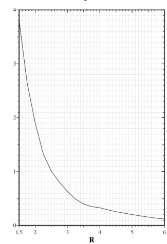
Fig. 2. The ILAT speed of the Polar satellite footpoint in the
iono-sphere, transformed to km/s (solid).
of the higher coarsening levels as well. Usually only one of the multiple found minima survives the postprocessing step, which is what one wants. Naturally, the act of deciding which minima are close enough to be considered equivalent is a sub-jective one. We think, however, that applying some sort of multiple minima removal method is much better than apply-ing none at all, for example, because in the latter case narrow minima would be found at many coarsening levels and thus be statistically overrepresented. We have also checked that changing the criteria within a reasonable range does not ap-preciably affect the statistical results.
3.3 Postprocessing steps
Before plotting and generating the statistical results pre-sented below, some further simple filtering conditions are ap-plied, which are listed here:
1. The angle between the ionosphere-projected satellite trajectory with constant ILAT circles must be between
60◦ and 120◦. This is done to remove passes where the
satellite moves nearly tangential to the auroral oval be-cause in such geometries, the satellite ILAT speed is low and the geometry is unfavourable for analysing the trajectory-integrated potential.
2. The angle between B and the satellite velocity vector
must be at least 30◦, because if the satellite moves
al-most parallel to the field line, the ILAT speed is again low and temporal variations easily interfere with the analysis.
3. Only events with a depth larger than 0.5 kV are shown, unless otherwise noted. The number of potential min-ima grows rapidly if one reduces the lower depth thresh-old.
In order to display statistical results, the orbital coverage is
needed as a function of altitude, MLT, Kp, and season. Since
we are expecting to measure static structures that the orbit in-tersects, it makes more sense to define the orbital coverage as the number of oval crossings rather than as the time spent. As the altitude in general varies somewhat as the satellite moves
between 64◦ and 75◦ ILAT, one has to decide which altitude
is defined as the altitude of the oval crossing. Notice that we cannot use the altitude at which the potential minimum is truly observed because there are usually several (or none at all) potential minima per oval crossing and the orbital cover-age must be computed in a way which is independent of the occurrence of the minima. We choose to define the altitude of the oval crossing to be the altitude where the satellite was when it crossed the nominal Q=2 oval in Table 1 of Holz-worth and Meng (1975).
3.4 Structure lifetime and motion effects
The ILAT speed of Polar is highly dependent on altitude and
is about 0.002◦ per s at R=5RE(Fig. 2). With this speed, it
takes about 50 s to pass through a potential minimum of 0.1◦
width. This time is shorter than typical lifetimes of auroral arcs, so the satellite does not miss such structures because of structure lifetime effects. Some of the widest minima
con-sidered in this study (0.6◦) could be possibly affected at high
altitudes, since it takes about 5 min to traverse through them, but we think that this cannot distort the statistics in a signifi-cant way.
The possibility that arc motion could affect the result is now considered. There are three possible cases: 1) The po-tential structure is moving towards the satellite. In this case the width and depth of the potential structure are underesti-mated, but their ratio (the effective electric field) is not af-fected. However, if the depth is underestimated so much that it drops below our selected threshold (0.5 kV), the struc-ture drops out of the database and in this way the effective electric field statistics are also affected. 2) The potential structure moves in the same direction as the satellite with an speed which is lower than the satellite speed. In this case the width and depth of the potential structure are overesti-mated, but again, the effective electric field is not affected. However, weak potential structures, that in reality are below the threshold, can be raised above the threshold and thus also affect the effective electric field statistics. 3) The potential structure moves in the same direction as the satellite with a speed which is larger than the satellite speed. In this case the
0 0.5 1 posprob=0 0 0.5 1 posprob=0.25 0 0.5 1 posprob=0.5 2 3 4 5 R/R_E 0 0.5 1 posprob=0.75
Occ. freq of Ei>100 mV/m, v=100 m/s
a
b
c
d
0 0.5 1 posprob=0 0 0.5 1 posprob=0.25 0 0.5 1 posprob=0.5 2 3 4 5 R/R_E 0 0.5 1 posprob=0.75Occ. freq of Ei>100 mV/m, v=200 m/s
a
b
c
d
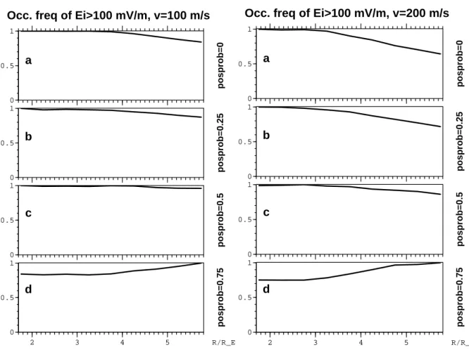
Fig. 3. Simulated effect of structure motion to effective mapped-down electric field occurrence frequency as a function of radial distance,
taking into account realistic Polar satellite speed at different altitudes. Panels (a)–(d) correspond to 0%, 25%, 50% and 75%, respectively, of the true potential structures being positive (black aurora structures). In the left plot the average structure speed in the ionosphere is 100 m/s and in the right plot it is 200 m/s.
polarity of the potential structure will come out reversed: a negative structure appears as a positive one and vice versa. Whether this causes a net underestimation or overestimation of the occurrence frequency of effective electric fields de-pends on the relative occurrence frequencies of negative and positive structures, which is unknown.
In summary, for structures that move slower than the satellite, the effects that occur for structures moving opposite or parallel to the satellite, at least qualitatively, tend to cancel each other out. Overall, some underestimation of the poten-tial structure occurrence frequency takes place if the struc-tures are fast-moving; exactly how much depends on how many positive potential structures there are. Concerning the effective electric field distribution of detected potential struc-tures, their distribution is essentially independent of the ve-locity of the structures.
To evaluate structure motion effects more quantitatively, we perform the following simple Monte Carlo simulation. As random variables we use (i) the potential structure depth
V, which is exponentially distributed, (ii) the potential
struc-ture ionospheric width, which obeys a uniform distribu-tion between 0 and 60 km, and (iii) the ionospheric
veloc-ity of the structure v, which is exponentially distributed with
v0=100 m/s or 200 m/s expectation value and a random sign.
The potential depth V is modified by the factor |vs|/|v − vs|,
where vs is the satellite speed (a realistic speed specific to
each altitude is employed, Fig. 2) and multiplied by −1, if v
and vs have the same sign and |v|>|vs|.
The results of the simulation are shown in Fig. 3. In the left plot the mean ionospheric speed of the structure is 100 m/s and in the right plot it is 200 m/s. To our knowledge, no large statistical studies of auroral arc speeds exist, but in event studies the speeds are mostly below 200 m/s, although speeds up to 400–500 m/s can also occur (Haerendel et al., 1993; Williams et al., 1998; Trondsen and Cogger, 2001); thus, the values 100 and 200 m/s shown in the plot pair of Fig. 3 should be representative. Notice that since the speeds are exponen-tially distributed, there are also much higher speeds than 200 m/s present in the simulated ensemble of potential structures. The quantity plotted in each panel of Fig. 3 is the number of negative potential structures reported by the simulated satel-lite at each altitude, divided by the true number of them. In panels (a) all the potential structures in the ensemble are as-sumed negative. At low altitude the satellite correctly detects
12 18 0 6 12 1 2 3 4 5 6
MLT
R
Fig. 4. All potential minima larger than 2 kV and with width <0.6◦(60 km in the ionosphere) as a function of MLT and radial distance R. Different energies (minimum depths) are shown by different symbols: 2–4 kV plus sign, 4–6 diamond, 6–8 small black disk, more than 8 large black disk.
all of them (the occurrence frequency is 1), but at high alti-tude it fails to detect those structures that move in the same direction as the satellite with a higher, speed because it mis-interprets them as positive structures. The effect is most pro-nounced in the right plot because there the structure speed is two times higher, on the average. In panels (b–d), some fraction of the structures in the ensemble are assumed to be positive (25%, 50% and 75%, respectively). We believe that values around 50% (panel (c)) are the most likely. Those pos-itive structures that move in the same direction as the satellite with a higher speed are now misinterpreted as negative ones and thus, they increase their reported number, partly or com-pletely balancing the effect. If the number of positive and negative structures is the same (panel (c)), the net influence
of the structure speed to the number of detected structures is almost nonexistent. The conclusion that we draw from Fig. 3 is that the structure motion effect on the occurrence frequency of effective electric fields is likely to be
negligi-ble below 4 RE radial distance and about 10–20% at 6 RE.
In the worst case (v0=200 m/s, no positive structures at all),
the effect would be about 40% at 6 REand negligible below
3.5 RE.
3.5 Effect of mapping
As mentioned above, we use the dipole ILAT throughout the paper. The employed ILAT definition has some effect to the structure width in the ionosphere, because the mapping de-pends on the underlying magnetic field model. To evaluate
64 70 75 1 2 3 4 5 6
ILAT
R
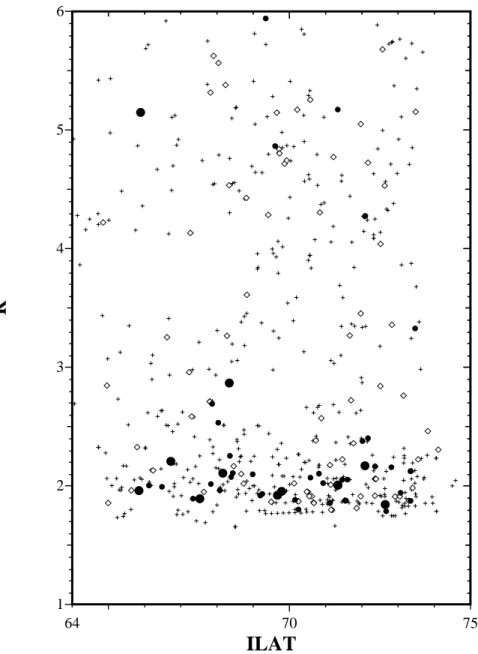
Fig. 5. Distribution of the minima against ILAT and R for the nightside (18:00–06:00 MLT) events. For details of the symbols, see caption
of Fig. 4.
the effect quantitatively, we check how much the structure widths would differ if the Tsyganenko–89 magnetic field model, together with IGRF internal field model, are used in-stead of a dipole model. The result is that in 50% of the cases, the difference is less than 11%, and in 90% of the cases it is less than 33%. Almost the same numbers are obtained
re-gardless of which Kpvalue (1–6) one uses in the Tsyganenko
model; thus, we conclude that the magnetic field model used to define the ILAT does not have a significant effect on our results.
Another effect of mapping is that ILAT values below 66
map below R=6 REin the equatorial plane. In other words,
in the highest radial distance bin (5.5 RE<R<6 RE), the
lowest ILAT values are not covered by the satellite. In
principle, this may distort the statistics in the highest radial
distance bin to some extent, although the effect should be rather minor since usually ILAT below 66 represents subau-roral latitudes where potential structures do not exist. The conclusions of the paper are not affected since they do not depend on the data in the highest radial distance bin.
4 Results for potential minima and their associated electric fields
As an overview, Fig. 4 shows all potential minima deeper than 2 kV as a function of MLT and radial distance R. Dif-ferent symbols indicate the depth of the minima (see fig-ure caption for details). Most potential minima are found at 18:00–04:00 MLT and the highest energy potential minima
a 0 100 200 300 400 500 600 Orb.coverage b 0 5 10 kV c 0 1 2 3 4 5 6 7 V/m d 0 0.5 1 Freq >0.1 V/m e 2 3 4 5 6 R/R_E 0 0.1 0.2 0.3 0.4 Freq >0.5 V/m
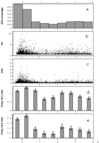
Fig. 6. All nightside potential minima deeper than 0.5 kV and the
corresponding effective ionospheric electric fields Ei: (a) number
of orbital crossings in each radial bin, (b) depth in kilovolts and radial distance of each potential minimum, (c) effective ionospheric electric field associated with each potential minimum with lower limit 100 mV/m, (d) occurrence frequency of Ei being larger than 100 mV/m (number of points in panel (c) divided by panel (a), (e) occurrence frequency of Ei being larger than 500 mV/m.
are found at low altitudes, below 3 RE. Similarly, Fig. 5
dis-plays the minima as a function of ILAT and R for the night-side (18:00–06:00 MLT). The potential minima tend to occur uniformly over the 65–74 ILAT range, partially because no MLT separation was done here (both the intrinsic variability and the dependence of the mean auroral oval on MLT con-tribute to the spreading of the distribution). Notice that in Figs. 4 and 5, the time spent by the satellite in different re-gions is not taken into account. In the subsequent plots the orbital coverage will be taken into account.
4.1 Altitude
Our baseline plot is Fig. 6 that shows results for all data
col-lected in the nightside including all Kp values. Panel (a) is
the number of orbital crossings in each 0.5 RE radial bin.
Panel (b) shows the depth in kilovolts of all found
poten-tial minima which are deeper than 500 V and at most 0.6◦
wide in ILAT (corresponding to 60 km in the ionosphere). Panel (c) shows the effective mapped-down ionospheric
elec-a 0 100 200 300 400 500 600 Orb.coverage b 0 5 10 kV c 0 1 2 3 4 5 V/m d 0 0.05 0.1 0.15 Freq >0.1 V/m e 2 3 4 5 6 R/R_E 0 0.01 0.02 0.03 0.04 0.05 0.06 0.07 Freq >0.5 V/m
Fig. 7. Same as Fig. 6 but only potential minima deeper than 3 kV
are included.
tric field Ei in V/m, associated with all those potential
min-ima plotted in the previous panel that also satisfy the
con-dition Ei>100 mV/m. The effective mapped-down
iono-spheric electric field is defined as the depth of the poten-tial minimum divided by the mapped-down half-width of the structure in the ionospheric plane. Notice that the effective
electric field Ei does not really exist in the ionosphere, but
we use the ionosphere just as a convenient reference altitude in order to easily compare electric fields measured at differ-ent altitudes. This variable is supposed to be invariant with radial distance above the acceleration region, if the accelera-tion structure is not local but is mapped along magnetic field lines towards the magnetosphere. Panel (d) is the occurrence
frequency of Ei>100 mV/m per orbital crossing, which is
obtained by dividing the number of data points in panel (c) in each radial bin by the corresponding orbital crossing number from panel (a) (so “1” means that there is one event every
orbit, on the average). The error bars correspond to 1/√n
relative errors, where n is the number of datapoints exceed-ing the threshold. Panel (e) is the occurrence frequency of
Ei>500 mV/m. Panels (d) and (e) should, in principle, be
divided by one of the profiles of simulated Ei occurrence
frequency displayed in Fig. 3. Applying such a correction would change the results only mildly in the highest radial distance bins, however.
a 0 50 100 150 200 250 Orb.coverage b 0 5 10 kV c 0 1 2 3 4 V/m d 0 0.5 1 1.5 2 Freq >0.1 V/m e 2 3 4 5 6 R/R_E 0 0.1 0.2 0.3 0.4 0.5 0.6 Freq >0.5 V/m a 0 100 200 300 400 Orb.coverage b 0 5 10 kV c 0 1 2 3 4 5 6 7 V/m d 0 0.5 1 1.5 2 Freq >0.1 V/m e 2 3 4 5 6 R/R_E 0 0.1 0.2 0.3 0.4 0.5 0.6 Freq >0.5 V/m
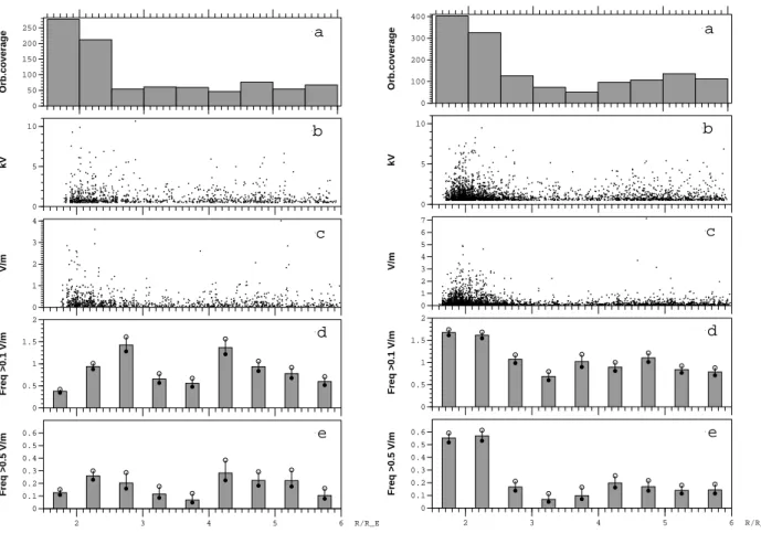
Fig. 8. Same as Fig. 6, but only when the ionosphere at satellite footpoint is sunlit (left plot) and in darkness (right plot).
We see from Fig. 6 (panels (d) and (e)) that the large ef-fective electric fields associated with potential minima oc-cur more frequently at low altitudes than at higher altitudes. The effect is quite pronounced in panel (e), i.e. when the threshold is 500 mV/m. A similar trend can also be seen in the scatter plot of the potential minima (panel (b)). We will see below (Sect. 4.3) that the increase in the occurrence
frequency above 4 RE is mainly due to phenomena in the
midnight MLT sector. Interestingly, an occurrence minimum
appears at 3–4 RE radial distance. Even though the figure
contains all nightside MLT and Kpvalues, this tends to
sug-gest that a simple mapping of the potential upward does not happen in the auroral zone.
In Fig. 7 we show the statistics of only those potential min-ima that are deeper than 3 kV. The trends seen in the baseline plot (Fig. 6) appear in Fig. 7 in a more dramatic form. Now we can distinguish two separate populations of potential
min-ima, and no events occur at 3–4 REradial distance in the
bot-tom panel, with only a few events in the 2nd panel from the bottom (see also the scatter plots).
4.2 Solar illumination dependence
In Fig. 8 we show the statistics separately for events when the ionosphere at the satellite footpoint is sunlit or in
dark-ness. During sunlit conditions (left panels), the maximum of the occurrence frequency of high potential minimum
associ-ated Ei fields (panel (d)) is shifted to a higher radial distance
(R=2.75 RE, corresponding to 11 000 km altitude from
Earth’s surface) than during darkness (R=1.75−2.25 RE,
the corresponding altitude is 5000–8000 km). Notice that we use numbers like 2.75 to uniquely label our bins, not to imply that the precision in altitude is two decimal digits. Further-more, in both sunlit and darkness cases separately, the max-imum occurrence frequency moves towards lower altitudes when the threshold is increased from 100 mV/m (panel (d))
to 500 mV/m (panel (e)). This means that strong Ei field
events tend to occur at lower altitudes. The overall occur-rence frequency is quite similar between sunlit and darkness for >100 mV/m events, but the low-altitude strong events (panel (e)) are clearly more common in shadow conditions; this may suggest that they tend to occur near local midnight, where the ionospheric footpoint is almost always in darkness. These results are in accordance with recent hybrid simula-tions of auroral potential structures (Janhunen and Olsson, 2002, Table 2). Both Fig. 8 and the simulations are consis-tent with the idea that sunlight increases the plasma density at low altitudes due to increased ionospheric photoionisation, which makes the bottom of the acceleration region move up-ward. This idea was first suggested by Bennett et al. (1983)
a 0 50 100 Orb.coverage b 0 5 10 kV c 0 0.5 1 1.5 2 2.5 3 V/m d 0 0.5 1 1.5 2 2.5 3 3.5 Freq >0.1 V/m e 2 3 4 5 6 R/R_E 0 0.5 1 1.5 Freq >0.5 V/m a 0 50 100 Orb.coverage b 0 5 10 kV c 0 1 2 3 4 V/m d 0 0.5 1 1.5 2 2.5 3 3.5 Freq >0.1 V/m e 2 3 4 5 6 R/R_E 0 0.5 1 1.5 Freq >0.5 V/m a 0 50 100 Orb.coverage b 0 5 10 kV c 0 1 2 3 V/m d 0 0.5 1 1.5 2 2.5 3 3.5 Freq >0.1 V/m e 2 3 4 5 6 R/R_E 0 0.5 1 1.5 Freq >0.5 V/m a 0 50 100 150 Orb.coverage b 0 5 10 kV c 0 0.5 1 1.5 2 2.5 3 V/m d 0 0.5 1 1.5 2 2.5 3 3.5 Freq >0.1 V/m e 2 3 4 5 6 R/R_E 0 0.5 1 1.5 Freq >0.5 V/m a 0 50 100 Orb.coverage b 0 5 10 kV c 0 1 2 3 4 5 6 7 V/m d 0 0.5 1 1.5 2 2.5 3 3.5 Freq >0.1 V/m e 2 3 4 5 6 R/R_E 0 0.5 1 1.5 Freq >0.5 V/m a 0 50 100 150 Orb.coverage b 0 5 10 kV c 0 1 2 3 V/m d 0 0.5 1 1.5 2 2.5 3 3.5 Freq >0.1 V/m e 2 3 4 5 6 R/R_E 0 0.5 1 1.5 Freq >0.5 V/m
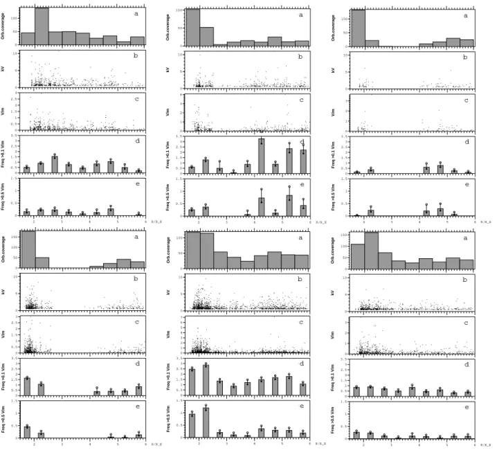
Fig. 9. Same as Fig. 6, but separated in dusk (18:00–22:00), midnight (22:00–02:00) and dawn (02:00–06:00) magnetic local time (MLT)
bins, as well as sunlit (top row) and darkness (bottom row) conditions. As in Fig. 6, all Kpvalues are included, width is restricted to be
smaller than 0.6◦and depth more than 0.5 kV.
based on S3–3 data. Figure 8 suggests that not only the ac-celeration region bottom altitude moves up, but also potential minima of given depth are rarer during sunlit conditions. In a particular model calculation of the hybrid simulation it was found that halving the ionospheric plasma density changed the potential depth from 3 kV to 3.7 kV, and the bottom alti-tude moved down from 5500 km to 2600 km (Janhunen and Olsson (2002), Table 2). Observationally it has also been found using satellite particle data that sunlight suppresses au-roral acceleration events (Newell et al., 1996).
4.3 MLT
From Fig. 4 it was seen that the potential minima are mainly found in the evening and midnight sectors. To study the MLT distribution in more detail, Fig. 9 shows the statistics separated in three nightside MLT bins (18:00–22:00, 22:00– 02:00, 02:00–06:00) and separated according to the footpoint illumination conditions.
For the lowest two or three altitude bins we have a reason-able orbital coverage in all six subplots (see the top panels in all subplots) and the behaviour can be summarised as fol-lows. In sunlit conditions, the occurrence frequency is about two times higher in the evening and midnight sectors than
a 0 100 200 300 400 Orb.coverage b 0 5 10 kV c 0 1 2 3 4 5 6 7 V/m d 0 0.5 1 1.5 2 Freq >0.1 V/m e 2 3 4 5 6 R/R_E 0 0.1 0.2 0.3 0.4 0.5 0.6 Freq >0.5 V/m a 0 50 100 150 200 250 Orb.coverage b 0 5 10 kV c 0 1 2 3 4 5 V/m d 0 0.5 1 1.5 2 Freq >0.1 V/m e 2 3 4 5 6 R/R_E 0 0.1 0.2 0.3 0.4 0.5 0.6 Freq >0.5 V/m
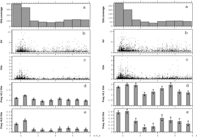
Fig. 10. Same as Fig. 6, but decomposed into small Kp(Kp≤2, left plot) and large Kp(Kp>2, right plot).
in the morning sector. In darkness conditions the highest occurrence frequency is found in the midnight sector, the occurrence frequencies are lower by a factor of 2–3 in the evening sector and the lowest frequencies appear again in the morning sector. These findings are in agreement with ear-lier studies concerning the occurrence of inverted-V events at low altitude (Lin and Hoffman, 1982). Overall, the occur-rence frequencies in darkness conditions are higher than in sunlit conditions.
For the high altitude bins (R>4 RE), the data coverage
is enough to draw some conclusions. The occurrence fre-quencies are highest in the midnight sector, both in sunlit and darkness conditions. Instead, in the evening and morn-ing sectors the occurrence frequencies are about equal, which is not the case in the low-altitude events.
Interestingly, the middle altitude occurrence frequencies
(R=3−4 RE) are smaller than the low and high altitude ones
in all cases where we have enough data to judge. Such a judgement can be done in the midnight sector for both sun-lit and darkness cases, as well as in the evening sector sunsun-lit case and the morning sector darkness case. Such a feature tends to suggest that the low-altitude and high-altitude struc-tures are not necessarily connected.
4.4 Kp
Kp-decomposed statistics are shown in Fig. 10. For the
low-altitude events the occurrence frequency is about two times
larger for Kp>2 than for Kp≤2; also, a bin at 2.75 RE
con-tains many events during high Kp. So the spatial length of
the low-altitude potential minimum region may increase with
increasing Kp. For the high-altitude events, the occurrence
frequency increases with increasing Kp; it is 3–4 times larger
for Kp>2 than for Kp≤2. Again, one should notice the
ex-istence of a minimum in occurrence rates at 3–4 RE radial
distance.
5 All electric fields
In the previous section we investigated how often potential minima occur in different regions. As the main measure, we used the effective mapped-down electric field associated with
the potential minimum, where the effective electric field Ei
was defined as the potential minimum depth divided by the mapped-down ionospheric half-width of the structure. To complement this, we now consider all perpendicular electric fields, not only those that are associated with potential min-ima. We still use the mapped-down version of the measured electric field to be able to easily compare different altitude observations.
0 500 1000 Orb. coverage 0 0.005 0.01 0.015 0.02 Occ. freq. >128 mV/m 0 0.001 0.002 0.003 0.004 0.005 0.006 0.007 0.008 Occ. freq. >256 mV/m 2 3 4 5 6 R/R_E 0 0.0005 0.001 0.0015 0.002 0.0025 Occ. freq. >512 mV/m
Fig. 11. Baseline plot of altitude distribution of mapped-down
per-pendicular electric field amplitudes Ei, including all fields not only those associated with potential minima: (a) number of orbital cross-ings in each radial bin, (b) occurrence frequency of Ei exceeding 100 mV/m, (c) occurrence frequency of Eiexceeding 500 mV/m.
5.1 Data processing
We take the measured electric field along the spacecraft tra-jectory and interpolate it to a fixed ILAT grid which has
∼10 m resolution in the ionosphere. Each auroral crossing
corresponds to 217data points. Using this high ILAT
resolu-tion ensures that we do not undersample the measured field, even at high altitude. The electric field is then multiplied by the ratio of the local satellite displacement divided by the displacement of the satellite footpoint in the ionosphere,
to obtain the mapped–down electric field Ei. Finally, Ei is
high-pass filtered so that ionospheric scale sizes above 60 km are removed. The filtering is done for consistency with the previous section results where our largest allowed size for potential minima was 60 km. The selection of data obeys the same rules as those described above for the potential minima, except that one need not remove the orbits quasi-parallel to the magnetic field.
5.2 Altitude
In Fig. 11 we show the baseline plot of the electric field al-titude distribution, which contains all nightside MLT-sectors
and all Kpvalues and illumination conditions. The top panel
is the number of orbital crossings. The second, third and fourth panels are the fraction of time (the occurrence
fre-quency, where “1” means that Ei is always larger than the
given threshold) when Ei exceeds 128, 256 and 512 mV/m,
respectively. Notice that the occurrence frequencies are now numerically much smaller than in the previous section, be-cause in that section the occurrence frequency was defined as the number per orbital crossings, not as a fraction of time,
as defined here. We see that large Ei fields peak at low
al-titudes, and there is a minimum at 3.75 RE. At higher
alti-tudes the fields again become stronger. These trends become clearer as the threshold is increased: at 128 mV/m threshold the distribution is still almost flat, but at 512 mV/m thresh-old the trends are clear. Both trends are similar to what
was observed for the potential minimum associated Ei fields
(Fig. 6). This suggests that potential minimum associated electric fields play an important role among all electric fields in the auroral zone. The error bars correspond to 1/
√
K
rela-tive errors, where K is the number of different orbital cross-ings having electric fields larger than the threshold. This cor-responds to assuming that all datapoints within one crossing are correlated, which need not be true, thus the error bars displayed should be considered as upper limits of the error.
5.3 Solar illumination
The sunlit/darkness decomposed statistics are shown in Fig. 12. We see that at low altitude the occurrence frequen-cies are about two times higher (at 512 mV/m) in darkness than in sunlit conditions. At high altitude there is not so
much difference. A radial shift of about one bin (0.5 RE)
can be seen in the low-altitude electric fields between sun-lit and darkness. Again, the occurrence rates of all electric fields have surprisingly similar profiles as those of the effec-tive electric fields related to potential minima in Fig. 8.
5.4 MLT
In Fig. 13 we decompose the Ei statistics in three MLT
sec-tors, as well as sunlit and darkness conditions. The high-altitude fields that occur in the baseline plot (Fig. 11) appear to come mainly from the midnight MLT sector. In all those MLT/illumination combination plots where we have enough orbital coverage to make a judgement (evening sunlit, mid-night sunlit, midmid-night darkness and morning darkness), there is a minimum in the occurrence frequency of strong
mapped-down electric fields around R=3.5 RE. Overall, the
occur-rence frequencies are largest in midnight and smallest in morning. A more detailed look reveals that interestingly, at low altitude the large electric fields are more common in the evening sector than in the morning sector, whereas at high al-titude they are equally common in the evening and morning sectors.
5.5 Kp
A comparison of low and high Kpvalues is shown in Fig. 14.
0 100 200 300 400 500 600 Orb. coverage 0 0.005 0.01 0.015 0.02 0.025 Occ. freq. >128 mV/m 0 0.005 0.01 Occ. freq. >256 mV/m 2 3 4 5 6 R/R_E 0 0.0005 0.001 0.0015 0.002 0.0025 0.003 0.0035 Occ. freq. >512 mV/m 0 100 200 300 400 500 600 Orb. coverage 0 0.005 0.01 0.015 0.02 0.025 Occ. freq. >128 mV/m 0 0.005 0.01 Occ. freq. >256 mV/m 2 3 4 5 6 R/R_E 0 0.0005 0.001 0.0015 0.002 0.0025 0.003 0.0035 Occ. freq. >512 mV/m
Fig. 12. Same as Fig. 11, but decomposed into sunlit ionospheric footpoint conditions (left) and darkness conditions (right).
about two times larger for high Kp than for low Kp. For
high-altitude electric fields, the transition from low to high
Kp brings about an even larger (about threefold) increase in
occurrence frequency, which is similar to the electric fields in the potential minima.
5.6 Scale size
In Fig. 15 we show the midnight darkness sector statistics for the effective electric field as a function of the mapped-down scale size (vertical axis). The scale size information is obtained by applying a running average with successively increasing window size and finding at each smoothing level how often the coarse-grained electric field exceeds the given threshold. Superimposed to the plots we also display two curves that correspond to the sampling rate of the instrument (20 samples per s in normal mode) and the spin frequency. The spin line has no significance, except that some spin con-tamination might be expected close to it or its harmonic mul-tiples, which we do not see here; however we propose that Fig. 15 shows three categories of electric fields: (1) back-ground electric fields that map along field lines, (2) electric fields of the arc-associated potential structures and (3) other electric fields whose spatio-temporal nature is uncertain. We propose that these categories manifest themselves in the fol-lowing way in Fig. 15. Background electric fields dominate the top panel, as is natural, since fields of ∼100 mV/m now
and then occur in the ionosphere and they vary slowly (i.e. above spin resolution). Arc-associated potential structure
electric fields are mainly seen as an island in the 2–2.5 RE
radial bin and above ∼1 km scale size. They are present in all panels, but one can distinguish them from the background fields most easily in the middle and bottom panels. Every-thing else seen in the plots is in the third category. At least part of these “other” electric fields are almost certainly asso-ciated with waves. Among the “other” electric fields are the high-altitude midnight sector fields mentioned several times earlier in this paper. They tend to peak, for example in 4–
5 RE bins in the bottom panel.
5.7 Orbital coverage
We have identified two clear populations of large electric
fields at ∼2 RE and 4–5 RE. We have considered possible
nongeophysical explanations and found two candidates that could cause the observed middle-altitude minimum in the oc-currence frequency. However, as we show below, they are not consistent with our data:
(1) The minimum could be caused by the satellite pass-ing through the altitude bin mostly in unfavourable ILAT. To check this, we plot in Fig. 16 the orbital coverage of Polar as a function of ILAT separately for all MLT sectors
and for three radial bins (2–3 RE, 3–4 RE and 4–5 RE,
0 50 100 150 200 250 Orb. coverage 0 0.01 0.02 0.03 0.04 0.05 Occ. freq. >128 mV/m 0 0.005 0.01 0.015 Occ. freq. >256 mV/m 2 3 4 5 6 R/R_E 0 0.001 0.002 0.003 0.004 0.005 0.006 Occ. freq. >512 mV/m 0 50 100 150 200 250 Orb. coverage 0 0.01 0.02 0.03 0.04 0.05 Occ. freq. >128 mV/m 0 0.005 0.01 0.015 Occ. freq. >256 mV/m 2 3 4 5 6 R/R_E 0 0.001 0.002 0.003 0.004 0.005 0.006 Occ. freq. >512 mV/m 0 50 100 150 200 250 Orb. coverage 0 0.01 0.02 0.03 0.04 0.05 Occ. freq. >128 mV/m 0 0.005 0.01 0.015 Occ. freq. >256 mV/m 2 3 4 5 6 R/R_E 0 0.001 0.002 0.003 0.004 0.005 0.006 Occ. freq. >512 mV/m 0 50 100 150 200 250 Orb. coverage 0 0.01 0.02 0.03 0.04 0.05 Occ. freq. >128 mV/m 0 0.005 0.01 0.015 Occ. freq. >256 mV/m 2 3 4 5 6 R/R_E 0 0.001 0.002 0.003 0.004 0.005 0.006 Occ. freq. >512 mV/m 0 50 100 150 200 250 Orb. coverage 0 0.01 0.02 0.03 0.04 0.05 Occ. freq. >128 mV/m 0 0.005 0.01 0.015 Occ. freq. >256 mV/m 2 3 4 5 6 R/R_E 0 0.001 0.002 0.003 0.004 0.005 0.006 Occ. freq. >512 mV/m 0 50 100 150 200 250 Orb. coverage 0 0.01 0.02 0.03 0.04 0.05 Occ. freq. >128 mV/m 0 0.005 0.01 0.015 Occ. freq. >256 mV/m 2 3 4 5 6 R/R_E 0 0.001 0.002 0.003 0.004 0.005 0.006 Occ. freq. >512 mV/m
Fig. 13. Same as Fig. 11, but decomposed into different MLT sectors (columns), as well as sunlit (top) and darkness (bottom) conditions.
perpendicularity requirements listed in Sect. 3.2 are included in Fig. 16. The orbital coverage decreases as a function of ILAT at all altitude bins and in all MLT sectors in a rather uniform way. No anomalously small coverage exists in the
3–4 REradial bin in the most probable auroral oval latitudes
as compared to the surrounding radial bins. The orbital cov-erage in Fig. 16 is plotted as the number of times that each
0.5◦ILAT bin is covered.
(2) The minimum could be caused by unfavourable solar
illumination, MLT, Kpor solar cycle phase during the times
the satellite probed the R=3.75 region. These factors can
be ruled out because the minimum is seen in all MLT, Kp
and season plots separately, and also because data at this altitude were gathered during many years. Most data for
3.75 RE come from 1999, which is a solar maximum year,
thus one would expect an even higher occurrence frequency
there because Kp is, on the average, higher. The fact that
Kpis higher can be seen for example by comparing the
sec-ond panels (the orbital coverages) of Fig. 10 at the R=3.75 bin. Furthermore, the minimum is found at slightly different
altitude for different Kp, which speaks in favour of a
geo-physical effect.
6 Summary
To find at which altitude auroral potential structures close, we have for the first time studied auroral electric fields in the
0 100 200 300 400 500 600 Orb. coverage 0 0.01 0.02 0.03 Occ. freq. >128 mV/m 0 0.005 0.01 Occ. freq. >256 mV/m 2 3 4 5 6 R/R_E 0 0.001 0.002 0.003 0.004 Occ. freq. >512 mV/m 0 100 200 300 400 500 600 Orb. coverage 0 0.01 0.02 0.03 Occ. freq. >128 mV/m 0 0.005 0.01 Occ. freq. >256 mV/m 2 3 4 5 6 R/R_E 0 0.001 0.002 0.003 0.004 Occ. freq. >512 mV/m
Fig. 14. Same as Fig. 11, but decomposed into small Kp(Kp≤2, left) and large Kp(Kp>2, right).
database of the Polar satellite covering five years. From the analysis we conclude that there are two separate classes of electric field structures that are seen as potential minima by a satellite traversing them. The first class is the low-altitude potential minima which are associated with inverted-V elec-tron spectra, auroral cavities and optical discrete arcs. These low-altitude potential minima are most often seen in the mid-night and evening MLT sectors, and their altitude moves
upward by ∼0.5−1 RE when the ionospheric footpoint
be-comes Sun-illuminated. The strongest structures (in terms
of their effective mapped-down ionospheric fields Ei) reside
at the lowest altitudes, and the structures are about twice as
common for Kp>2 than for Kp≤2.
Another class of electric field structures resides at high
al-titude (R>4 RE) in the midnight MLT sector. To some
ex-tent they also occur in the evening sector. This class of elec-tric field structures is also a new finding of this paper, and their nature is still unknown to us. Since they occur
predom-inantly in the midnight MLT sector and react to Kp more
strongly than the low-altitude fields, they are probably super-posed substorm-related processes. They need not necessarily be quasi-static potential well structures in the same sense as the low-altitude ones, but could also correspond to tempo-rally evolving structures (potential or inductive). Since the satellite ILAT speed is low at high altitudes, structures which oscillate in the north-south direction at a sufficiently rapid
pace can encounter the satellite multiple times which may partly be the explanation for their relatively high occurrence frequency.
Equally interesting as the existence of the two classes of electric field structures is the relative rarity of the structures
in middle altitudes (R=3−4 RE). In principle, concerning
the potential structure closure question, two interpretations are possible:
1. The low-altitude potential structures do not extend be-yond middle altitudes, which necessitates the existence of downward parallel electric fields in the intermedi-ate region (Janhunen et al., 1999; Janhunen and Ols-son, 2000, 2001, 2002; Hallinan and Stenbaek-Nielsen, 2001);
2. The low-altitude narrow structures widen before reach-ing higher altitudes so that the effective electric fields associated with them are reduced (Mozer and Hull, 2001).
The first possibility is called the Cooperative Model (for a recent review, see Olsson and Janhunen, 2003) and the lat-ter possibility is called the potential finger model. In
nei-ther model can the structures above 4 RE be related to the
electrostatic potential structures of the auroral region. Fig-ure 17 shows schematically the closed potential structFig-ure in the Cooperative Model for quiet arcs (top) and superposed
20 ss/s Spin 0.01 0.1 1 10 Scale (km) Occ.freq >128 mV/m 10−4 10−3 0.01 20 ss/s Spin 0.01 0.1 1 10 Scale (km) Occ.freq >256 mV/m 10−4 10−3 0.01 20 ss/s Spin 2 3 4 5 6 R/R_E 0.01 0.1 1 10 Scale (km) Occ.freq >512 mV/m 10−4 10−3 0.01
MLT 22−02, Darkness
Fig. 15. Occurrence frequency of mapped-down effective
elec-tric field exceeding threshold 128 mV/m (top), 256 mV/m (second panel) and 512 mV/m (bottom), as a function of radial distance and mapped-down ionospheric scale size. Curves corresponding to satellite spin frequency 1/6 Hz and normal 20 samples per second are superposed. Data below the 20 Hz curve do not carry physical information and are thus shown as white.
with a substorm-time high-altitude electric field structure in the midnight MLT sector (bottom). The nature of the high-altitude fields is an open question. They could be electric fields of Alfv´en waves or they could be quasi-electrostatic structures created at that altitude, for example by a Landau resonance between Alfv´en waves and electrons.
To open up a new viewpoint to the data we also investi-gated the altitude statistics of all electric fields, not only those associated with potential minima. The results are similar to the potential structure results in all important ways. This sug-gests that the statistical results presented in this paper are not caused by problems in the minimum finding algorithm and that electric fields associated with potential structures are the most important class of electric fields found on auroral field lines.
A recent study of auroral density depletions shows that the depletions are concentrated mostly at low altitudes, however, with another island of high-altitude depletions appearing in the midnight MLT sector (Janhunen et al., 2002). This al-titude pattern is very similar to the potential structure
pat-0 100 200 300 400 500 600 700 800 18−22 0 100 200 300 400 500 600 700 800 # of 0.5deg ILAT 22−02 65 66 67 68 69 70 71 72 73 74 ILAT 0 100 200 300 400 500 600 700 800 02−06 Orbital coverage, R=2−3 0 50 100 150 200 250 300 18−22 0 50 100 150 200 250 300 # of 0.5deg ILAT 22−02 65 66 67 68 69 70 71 72 73 74 ILAT 0 50 100 150 200 250 300 02−06 Orbital coverage, R=3−4 0 100 200 300 400 500 18−22 0 100 200 300 400 500 # of 0.5deg ILAT 22−02 65 66 67 68 69 70 71 72 73 74 ILAT 0 100 200 300 400 500 02−06 Orbital coverage, R=4−5
Fig. 16. Orbital coverage of Polar sectors satisfying our criteria of
enough perpendicular trajectory in three radial distance ranges and in the three nightside MLT sectors.
tern found in the present paper. Also, it has been shown that the occurrence frequency of upgoing ion beams has a dip
at 3.5–4 RE radial distance (Janhunen et al., 2003). Taken
together, these results are consistent with the idea that the negative low-altitude potential structures correspond to den-sity depletions. The working of the concept has also been demonstrated with a hybrid simulation (Janhunen and Ols-son, 2002).
Fig. 17. Schematic figure containing the potential structure in the
Cooperative Model for stable arcs (top), the same with a superposed high-altitude substorm-time electric field structure in the midnight MLT sector (bottom).
Acknowledgements. We are grateful to F. S. Mozer for providing
the EFI data. We also thank C. T. Russell for providing MFE data. The work of PJ was supported by the Academy of Finland and that of AO by the Swedish Research Council. We are grateful to Andris Vaivads for useful comments of the manuscript.
The Editor in Chief thanks T. Hallinan and two other referees for their help in evaluating this paper.
References
Bennett, E. L., Temerin, M., and Mozer, F. S.: The distribution of auroral electrostatic shocks below 8000-km altitude, J. Geophys. Res., 88, 7107–7120, 1983.
Borovsky, J.: Auroral arc thicknesses as predicted by various theo-ries, J. Geophys. Res., 98, 6101–6183, 1993.
Bryant, D. A. and Perry, C. H.: Velocity-space distributions of wave-accelerated auroral electrons, J. Geophys. Res., 100, 23 711–23 725, 1995.
Carlqvist, P. and Bostr¨om, R.: Space-charge regions above the au-rora, J. Geophys. Res., 75, 7140–7146, 1970.
Haerendel, G., Buchert, S., LaHoz, C., Raaf, B., and Rieger, E.: On the proper motion of auroral arcs, J. Geophys. Res., 98, 6087– 6099, 1993.
Hallinan, T. J., Kimball, J., Stenbaek-Nielsen, H. C., Lynch, K., Arnoldy, R., Bonnell, J., and Kintner, P.: Relation between op-tical emissions, particles, electric fields, and Alfv´en waves in a multiple rayed arc, J. Geophys. Res., 106, 15 445–15 454, 2001. Hallinan, T. J., and Stenbaek-Nielsen, H. C.: The connection be-tween auroral acceleration and auroral morphology, Phys. Chem. Earth, 26, 169–177, 2001.
Harvey, P., Mozer, F. S., Pankow, D., Wygant, J., Maynard, N. C., Singer, H., Sullivan, W., Anderson, P. B., Pfaff, R., Aggson, T., Pedersen, A., F¨althammar, C. G., and Tanskanen, P.: The electric field instrument on the Polar satellite, Space Science Reviews, 71, 583–596, 1995.
Holzworth, R. H. and Meng, C.-I.: Mathematical representation of the auroral oval, Geophys. Res. Lett., 2, 377–380, 1975. Janhunen, P., Olsson, A., Mozer, F. S ., and Laakso, H.: How does
the U-shaped potential close above the acceleration region? A study using Polar data, Ann. Geophysicae, 17, 1276–1283, 1999. Janhunen, P. and Olsson, A.: New model for auroral acceleration: O-shaped potential structure cooperating with waves, Ann. Geo-physicae, 18, 596–607, 2000.
Janhunen, P. and Olsson, A.: Auroral potential structures and current-voltage relationship: summary of recent results, Phys. Chem. Earth, 26, 107–111, 2001.
Janhunen, P., and Olsson, A.: A hybrid simulation model for a sta-ble auroral arc, Ann. Geophysicae, 20, 1603–1616, 2002. Janhunen, P., Olsson, A., and Laakso, H.: Altitude dependence of
plasma density in the auroral zone, Ann. Geophysicae, 20, 1743– 1750, 2002.
Janhunen, P., Olsson, A., and Peterson W. K.: The occurrence fre-quency of upward ion beams in the auroral zone as a function of altitude using Polar/TIMAS and DE-1/EICS data, Ann. Geo-physicae, 21, 2059–2072, 2003.
Knudsen, D. J., Donovan, E. F., Cogger, L. L., Jackel, B., and Shaw, W. D.: Width and structure of mesoscale optical auroral arcs Geophys. Res. Lett., 28, 705–708, 2001.
Lin, C. S. and Hoffman, R. A.: Observations of inverted-V electron precipitation, Space Sci. Rev., 30, 415–457, 1982.
Lindqvist, P.-A. and Marklund, G. T.: A statistical study of high-altitude electric fields measured on the Viking satellite, J. Geo-phys. Res., 95, 5867–5876, 1990.
Maggs, J. E. and Davis, T. N.: Measurements of the thicknesses of auroral structures, Planet. Space Sci., 16, 205, 1968.
McFadden, J. P., Carlson, C. W., Ergun, R. E., Mozer, F. S., Temerin, M., Peria, W., Klumpar, D. M., Shelley, E. G., Peter-son, W. K., Moebius, E., Kistler, L. , Elphic, R. , Strangeway, R., Cattell, C., and Pfaff, R.: Spatial structure and gradients of ion beams observed by FAST, Geophys. Res. Lett., 25, 2021–2024, 1998.
Moore, T. E., Chappell, C. R. , Chandler, M. O., Fields, S. A., Pol-lock, C. J., Reasoner, D. L., Young, D. T., Burch, J. L., Eaker, N., Waite Jr., J. H., McComas, D. J., Nordholt, J. E., Thomsen, M. F., Berthelier, J. J., and Robson, R.: The Thermal Ion Dynamics Experiment and Plasma Source Instrument, Space Sci. Revs., 71, 409, 1995.
Mozer, F. S., Carlson, C. W., Hudson, M. K., Torbert, R. B., Parady, B., Yatteau, I., and Kelley, M. C.: Observations of paired elec-trostatic shocks in the polar magnetosphere, Phys. Rev. Lett., 38, 292, 1977.
Mozer, F. S., Cattell, C. A., Hudson, M. K., Lysak, R. L., Temerin, M., and Torbert, R. B.: Satellite measurements and theories of low altitude auroral particle acceleration, Space Sci. Rev., 27, 155–213, 1980.
Mozer, F. S. and Hull, A.: Origin and geometry of upward parallel electric fields in the auroral acceleration region, J. Geophys. Res., 106, 5763–5778, 2001.
Newell, P. T., Meng, C.-I., and Lyons, K. M.: Suppression of dis-crete aurora by sunlight, Nature 381, 766–767, 1996.
Olsson, A. and Janhunen, P.: Some recent developments in un-derstanding auroral electron acceleration processes, IEEE Trans. Plasma Sci., in press, 2004.
Russell, C. T., Snare, R. C., Means, J. D., Pierce, D., Dearborn, D., Larson, M., Barr, G., and Le, G.: The GGS/Polar Magnetic Fields Investigation, Space Sci. Rev., 71, 563–582, 1995.
Stenbaek-Nielsen, H. C., Hallinan, T. J., Osborne, D. L., Kimball, J., Chaston, C., McFadden, J., Delory, G., Temerin, M., and Carlson, C. W.: Aircraft observations conjugate to FAST: auroral arc thickness, Geophys. Res. Lett., 25, 2073–2076, 1998. Torbert, R. B. and Mozer, F. S.: Electrostatic shocks as the source of discrete auroral arcs, Geophys. Res. Lett., 5,, 135–138, 1978.
Trondsen, T. S. and Cogger, L. L.: Fine–scale optical observations of aurora, Phys. Chem. Earth, 26, 179–188, 2001.
Williams, P. J. S., del Pozo, C. F., Hiscock, I., and Fallows, R.: Velocity of auroral arcs drifting equatorward from the polar cap, Ann. Geophys., 16, 1322–1331, 1998.