THE DIURNAL CIRCULATION OF THE THERMOSPHERE
by
C. PABLO LAGOS
B. S., Universidad Nacional Mayor de San Marcos, Lima, Peru
(1964)
M. S., Massachusetts Institute of Technology (1967)
SUBMITTED IN PARTIAL FULFILLMENT REQUIREMENTS FOR THE DEGREE
DOCTOR OF PHILOSOPHY
OF THE OF
at the
MASSACHUSETTS INSTITUTE OF TECHNOLOGY (October, 1969)
Signature of Author... L ...
Department of Meteorology, 27 October 1969 Certified By...
, I Thesis Supervisor Accepted By ... .. . ... - ...
Chairman, Departme l Committee on Graduate Students
THE DIURNAL CIRCULATION OF THE THERMOSPHERE
by
C. Pablo Lagos
Submitted to the Department of Meteorology on 27 October 1969 in partial fulfillment of the requirement for the degree of Doctor of Philo sophy.
ABSTRACT
Two studies of the thermospheric physics and dynamics are considered. In the first study a comprehensive theoretical discussion of the nature of energy sources and of the general theory of gravity-tidal wave motions in the neutral gas is given. We con-sider motions which are of planetary scale in the horizontal and which have time scales of order of a day or longer. For time scale of one day we derive equations which generalize the usual equations for
atmospheric tides and may be used to describe the diurnal circulation of the thermosphere. Motions are classified as thermally, thermal--electromagnetically, and electromagnetically driven, according to which driving force is most important. Motions are further classified by the relative importance of viscosity and heat conduction as inviscid, transition, and diffusive regimes. For large ion drag, typical of high
solar activity, we define a "thermal geoplasma regime" which des-cribes the balance between the thermal forcing and the ion drag in the momentum equation. This motion regime is fully studied.
The dissipative processes of viscosity, heat conduction, and ion drag are briefly discussed. The physics of diabatic heating sour-ces as they occur in the thermosphere are discussed in some detail from the macroscopic and microscopic pointsof view. Ionization heating
efficiency for neutral particles is found to be as large as 85% and for electrons as low as 2% above 200 km. A simple and useful expression
for Joule heating in terms of neutral and drift velocities is derived. It is found that Joule heating, heating by viscous dissipation, corpus-cular heating, and chemical heating can only be as large as one tenth of solar heating.
In the second study the "thermal geoplasma motion regime" forced by solar heating and infrared cooling is integrated numerically in the forced region and analytically outside the forced region. The analytical study reduces to the solution of a fourth order ordinary diff-erential equation whose solutions are coefficients of spherical har-monics. Power series solutions satisfying the condition of no flux at z = " are obtained. Another solution satisfying the boundedness condition for small z is obtained in integral form. The two solutions are matched at the upper and lower boundaries of the numerical in-tegration region. The results further establish that adiabatic heating
and cooling by vertical motions is the "second heat source" of Harris & Priester.
Thesis Supervisor: Reginald E. Newell
TABLE OF CONTENTS
List of Figures List of Tables
PART I. THEORETICAL CONSIDERATIONS 1. INTRODUCTION
1. 1 The General Circulation of the Atmosphere-1. 2 Atmospheric Tides
1. 3 Motivation and Statement of the Problem 1. 4 Scope of the Present Study
2. THE DYNAMIC EQUATIONS WITH VISCOSITY, HEAT CONDUCTION, AND ION DRAG
2. 1 The Exact One-component Gas Dynamic Equations 2. 2 The One-component Gas Primitive Equations 3. THE NONDIMENSIONAL EQUATIONS
3. 1 Scaling Assumptions
3. 2 The Nondimensional Equations
4. CLASSIFICATION OF THE MOTION REGIMES 4. 1 The Nature of Nondimensional Parameters 4, 2 The Inviscid Regime
4. 4 The Viscous Regime
4. 5 The Thermal Geoplasma Regime 5. FORMULATION OF BOUNDARY CONDITIONS
5. 1 Lateral Boundary Conditions 5. 2 Vertical Boundary Conditions
6. THE PHYSICS OF VISCOSITY, HEAT CONDUCTION, AND ION DRAG COEFFICIENTS
1. 1 Viscosity
6. 2 Heat Conduction 6. 3 Ion Drag
7. THE PHYSICS OF DIABATIC HEATING 7. 1 Solar Heating
7. 2 Heating Efficiency in the Neutral Gas 7. 3 Heating Efficiency in the Ionosphere 7. 4 Infrared Cooling
7. 5 Heating and Cooling Rates
PART II. ANALYTICAL AND NUMERICAL STUDIES 8. THE CIRCULATION IN THE MIDDLE
THERMOS-PHERE: PROCEDURE
8: 1 General Remarks and Description of the Simple
8. 2 Representation of the System of Equations in Terms of Spherical Harmonics
8. 3 Formulation of Variables
8. 4 Analytical Solution and Discussion of Vertical Boundary Conditions
8. 4. 1 Discussion of the problem
8. 4. 2 Change of variables and asymptotic behaviour
8. 4. 3 Series solution
8. 4. 4 Integral representation and asymptotic behaviour
8. 4. 5 Matching solutions and determination of the model vertical boundary conditions
8. 5 Numerical Procedure
8. 6 A Justification of the Simple Case Study 9. RESULTS OF THE NUMERICAL STUDIES
9. 1 General Description of the Model Calculations 9, 2 Derivation of the Standard Data
9. 3 Results for Different Heating Efficiencies 9. 4 Results for Different Boundary Conditions 9. 5 Results for Various Electron Density Profiles
9. 6 Results for Changes in the Mean Temperature Field 9. 7 Results for Subsidence Heating
10. GENERAL DISCUSSION AND CONCLUSION 10. 1 Discussion of Velocity Field
10. 2 Discussion of Temperature Field
10. 3 The Significance of Adiabatic Heating by Vertical Motion
Acknowledgements References
Appendix I The Energy Equation for a Single Fluid Plasma Approximation
LIST OF FIGURES
Figure Page
Number Number
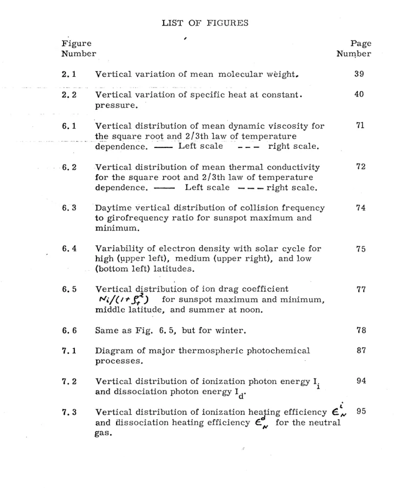
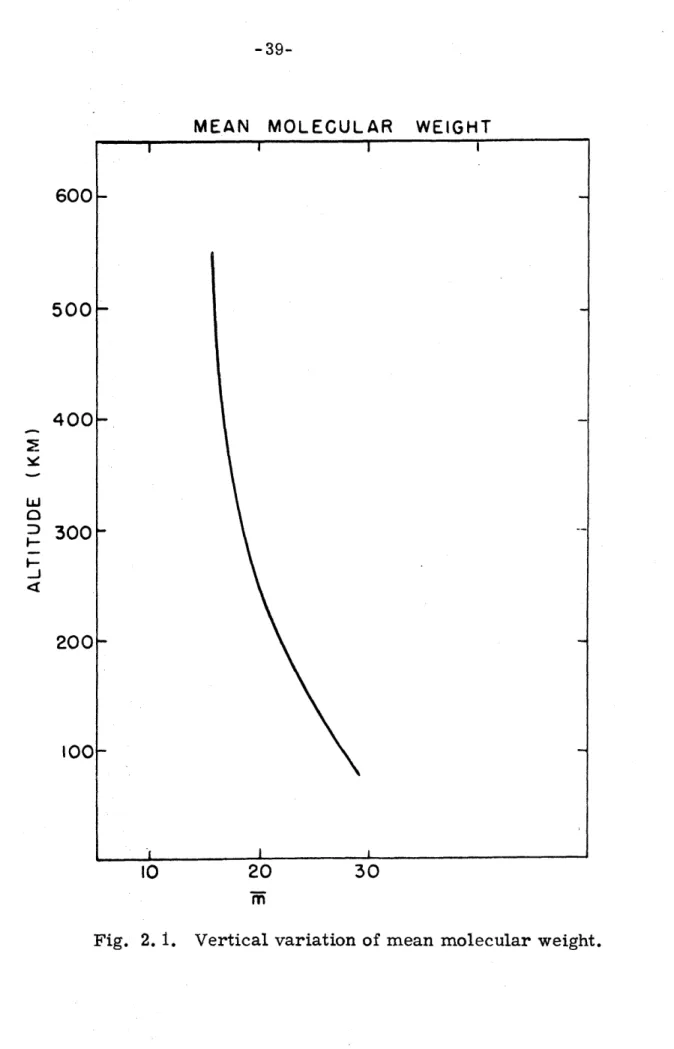
2. 1 Vertical variation of mean molecular weight. 39 2. 2 Vertical variation of specific heat at constant. 40
pressure.
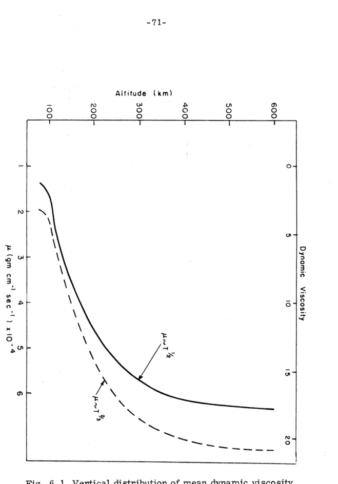
6. 1 Vertical distribution of mean dynamic viscosity for 71 the square root and 2/3th law of temperature
dependence. - Left scale - - right scale.
6. 2 Vertical distribution of mean thermal conductivity 72 for the square root and 2/3th law of temperature
dependence. Left scale - - - right scale.
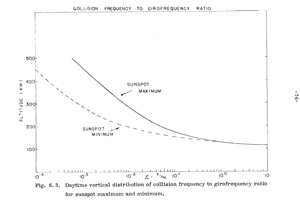
6.3 Daytime vertical distribution of collision frequency 74 to girofrequency ratio for sunspot maximum and
minimum.
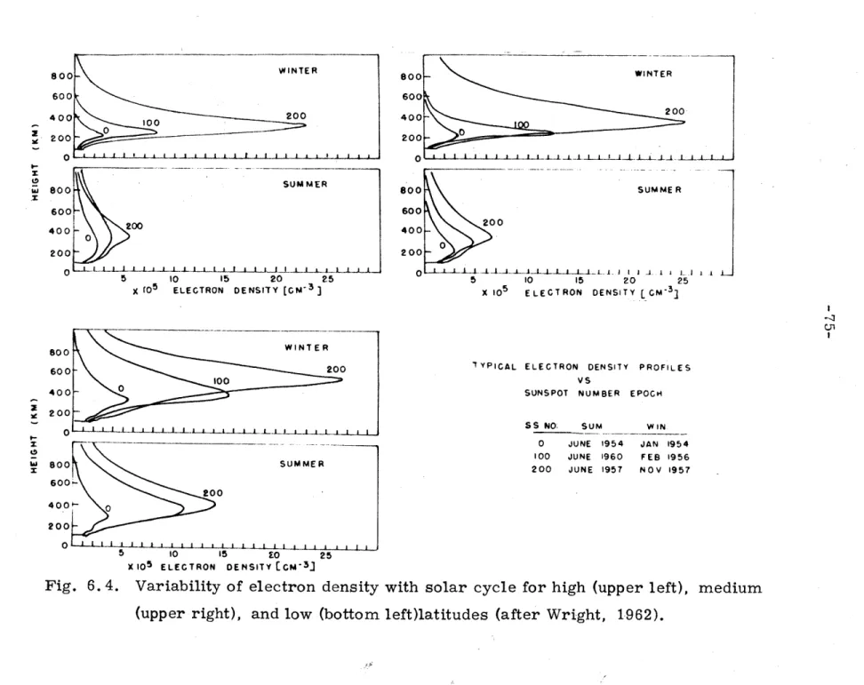
6. 4 Variability of electron density with solar cycle for 75 high (uipper left), medium (upper right), and low
(bottom left) latitudes.
6. 5 Vertical distribution of ion drag coefficient 77
M/(I
ff)
for sunspot maximum and minimum,middle latitude, and summer at noon.
6. 6 Same as Fig. 6. 5, but for winter. 78
7. 1 Diagram of major thermospheric photochemical 87 processes.
7.2 Vertical distribution of ionization photon energy I. 94 and dissociation photon energy Id
-7. 3 Vertical distribution of ionization heating efficiency . 95 and dissociation heating efficiency , for the neutral
Figure Page
Number Number
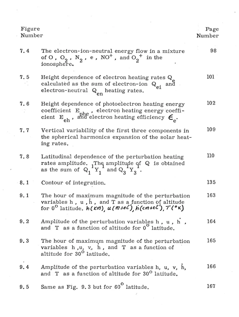
7.4 The electron-ion-neutral energy flow in a mixture 98 of O, 0 2 N2 , e, NO+ , and 02+ in the
ionosphere.
7. 5 Height dependence of electron heating rates Q 101 calculated as the sum of electron-ion
Q
ei anselectron- neutral Q heating rates. en
7. 6 Height dependence of photoelectron heating energy 102 coefficient E D , electron heating energy
coeffi-cient Eeh an electron heating efficiency E .
7. 7 Vertical variability of the first three components in 109 the spherical harmonics expansion of the solar
heat-ing rates.
7. 8 Latitudinal dependence of the perturbation heating 110 rates amplitude. 1Thi amplitu e qf Q is obtained
as the sum of Q1 Y and Q3 Y
8.1 Contour of integration. 135
9. 1 The hour of maximum magnitude of the perturbation 163 variables h, u , h , and T as a function of altitude
for 00 latitude. h(r*), u(a ec)r.se,,h(cMse) (oK)
9. 2 Amplitude of the perturbation variables h , u , h , 164 and T as a function of altitude for 0 latitude.
9. 3 The hour of maximum magnitude of the perturbation 165 variables h ,u, v, h, and T as a function of
altitude for 300 latitude.
9. 4 Amplitude of the perturbation variables h, u, v, h, 166 and T as a function of altitude for 300 latitude.
Figure Page
Number Number
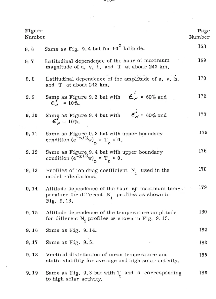
9. 6 Same as Fig. 9. 4 but for 600 latitude. 168 9. 7 Latitudinal dependence of the hour of maximum 169
magnitude of u, v, h, and T at abour 243 km.
9. 8 Latitudinal dependence of the amplitude of u, v, h, 170 and T at about 243 km.
9. 9 Same as Figure 9. 3 but with
6,
= 60% and 172 ,6 = 10%.9. 10 Same as Figure 9. 4 but with 6E = 60% and 173 E 10%.
9. 11 Same as Figure 9. 3 but with upper boundary 175 condition (e- z /2w) = T = 0.
z z
9.12 Same as Figure 9. 4 but with upper boundary 176 condition (e-/2w) = T = 0.
9. 13 Profiles of ion drag coefficient N. used in the 178 model calculations.
9. 14 Altitude dependence of the hour of maximum tem- 179 perature for different N. profiles as shown in
Fig. 9.13.
9. 15 Altitude dependence of the temperature amplitude 180 for different N. profiles as shown in Fig. 9. 13.
9.16 Same as Fig. 9. 14. 182
9.17 Same as Fig. 9. 5. 183
9. 18 Vertical distribution of mean temperature and 185 static stability for average and high solar activity.
9. 19 Same as Fig. 9. 3 but with T and s corresponding 186 to high solar activity.
Figure Page
Number Number
9. 20 Same as Fig. 9. 4 but with T and s corresponding 187 to high solar activity.
9. 21 Vertical distribution of the amplitude of adiabatic 189 heating by vertical motion corresponding to the
standard results.
9. 22 Latitudinal distribution of the amplitude of adiabatic 190 heating by vertical motion corresponding to the
stan-dard results.
10. 1 Vertical distribution of the hour of maximum tem- 199 perature when the subsidence heating is and is not
included in the standard model calculations.
10. 2 Vertical distribution of the temperature amplitude 200 when subsidence heating is and is not included in
the standard model calculations.
10. 3 Same as Fig. 10. 1 but for model calculation with 202 upper boundary conditions (e-z/ 2w) = T = 0.
LIST OF TABLES
Table Page
Number Number
-4 -1 -2
. Solar flux (e. v ) and cross section (10 gm cm ) 90 2. Atmospheric composition for medium solar activity, 92
1200 hours.
3. Pressure, mean heights, and height range for the 159 levels used in the model calculations.
4. Numerical values of ion drag parameters used in 177 the model calculations,
PART I. THEORETICAL CONSIDERATIONS 1. INTRODUCTION
1. 1 The General Circulation of the Atmosphere
The study of the general circulation of the atmosphere is the description and explanation of the characteristic properties of all circulation patterns which ever occur in the atmosphere.
The circulation patterns include the long-term time and zonally averaged circulations, synoptic features such as cyclones, anticyclones, and the jet streams, long and ultra-long waves, and tidal and gravity waves. From these, only the long-term and synoptic circulations have received more attention in the general circulation of the lower atmosphere. Long and ultra-long waves have received more attention in weather prediction. Because of a minor amount of the total energy contained in the tidal and gravity wave, they have not been considered at all in the general circulation of the lower atmosphere. Only in the thermosphere is the gravity-tidal motion a dominant feature.
The circulation pattern is described by the field of motion, temperature, radiation, and other thermodynamic variables.
There seems to be no question that the driving force of the circulation is the solar radiation. The absorption of this radiation takes place throughout the atmosphere. Most of the radiation lies
in the visible region and reaches the earth surface where it is absorbed and which in turn is transmitted to the overlying atmos-phere. The remaining solar energy in the ultraviolet, soft and hard x-rays, and infrared regions is absorbed by the atmospheric gases. Some of this energy is reflected or scattered back to space and plays no further role in the energy balance of the atmosphere.
The incoming solar energy is more intense in low than in high latitudes, and the net result is therefore a considerable excess of heating in low latitudes, which causes a cross-latitude pressure gradient. It follows that horizontal and vertical motions must develop and consequently the atmosphere possesses a circulation to allow a transport of energy across each latitude.
This circulation must possess a direct meridional cell to transport the required amount of energy poleward. Since this cell would also transport angular momentum poleward, there must be easterly surface winds in low latitudes and westerlies in higher lati-tudes. But such a single meridional cellular circulation is not
ob-served. The real atmosphere contains eddy structures which have been extensively described in the literature. The role of the eddies represent one of the most important aspects of the general circu-lation of the lower atmosphere. The energy of the eddies in the
form of available potential energy is gained from the zonally
averaged circulation by transporting energy toward latitudes of lower temperature, and kinetic energy is returned to the zonal flow by
eddies transporting angular momentum toward latitudes of higher angular velocity. The gain of kinetic energy from the eddies by the mean flow has been considered as a new physical phenomenon and discussed extensively by Starr (1968).
The description and explanation of the general features of the general circulation in the lower atmosphere as revealed by observation is discussed in detail by Lorenz (1967). Newell (1968) has reviewed and discussed the pertinent main features of the general circulation of the atmosphere above 60km.
1. 2 Atmospheric Tides
The formulation of the dynamical tidal theory in connection with the oscillation of the ocean and the lower atmosphere, where the dissipative effect of viscosity, heat conduction and ion drag can be neglected, was first presented by Laplace (1799, 1825). The
solution of the so-called Laplace's tidal equation has been extensively studied after the elegant treatment of Hough (1897, 1898), who first obtained solutions in terms of spherical harmonics. A detailed
review of the derivation and discussion of the tidal equations are given by Wilkes (1949) and Siebert (1961). The discussion includes both gravitational lunar tide and gravitational and thermal solar tides.
Further calculation and investigation of Laplace 's tidal equations are presented by Kato (1966), Lindzen (1966b, 1967b) and Longuet-Higgins (1967), among others. A somewhat different derivation of the class-ical atmospheric tidal equation has been presented by Dickinson (1966) and Flattery (1967), based on the primitive equations of meteorology. A more specialized article on lunar tides has been written by
Matsushita (1967).
The observed diurnal density variation in the thermosphere indicates that the oscillation has strong thermal origin, that is, the main thermal drive for the diurnal oscillation is the absorption of the extreme ultraviolet solar radiation. It will become clear from the present study that the theory of the diurnal bulge can be interpreted
as an extension of the diurnal tidal theory of the lower atmosphere.
1. 3 Motivation and Statement of the Problem
To begin with the study of the diurnal circulation of the thermosphere, one certainly would start with the description of the
general behaviour of the wind and temperature fields, and the neutral and ionized constituents. Having established from observation what the general features of the circulation are, one would proceed with theoretical studies searching for the explanation. To do this we would
employ our experience with the analogous circulation of the lower atmosphere or else we would develop new procedures to provide deeper physical insight to the problem at hand.
We would be, however, far behind if we followed systematically this procedure. There are practically no observations on a global
scale that can be used for obtaining the statistical properties of the circulation. A somewhat detailed picture of the fields of neutral gas density has only emerged from the analysis of satellite drag measure-ments above 100km. There is also some very scarce data on compo-sition and temperature obtained with high altitude rockets. The statistics of these data has revealed five different effects on the net-tral gas density, which are:
1) the diurnal variation
2) variation with geomagnetic activity 3) the 27-day variation
4) the semiannual variation 5) variation with solar cycle
Detailed discussion of these effects are given by Jacchia (1967), Jacchia and Slowey (1967), Keating and Prior (1967), Harris and Priester (1967), and Priester et al. (1967).
To attempt an explanation of the physical behavior of the thermosphere we further require the knowledge of the temperature and wind fields. The temperature can be derived from density fields, and the wind fields, due to lack of observations, can only be derived indirectly. Here we compute these fields theoretically and investi-gate their role. From our experience in dynamical meteorology we know that the thermosphere must possess a circulation, since a state of no motion would be incompatible with the poleward temperature gradient which radiative processes alone would demand. We expect that these large-scale motions will play a significant role in most of the problems that remain to be solved.
The present study, therefore, is motivated by the lack of the-oretical description which can explain properly several time-varying features of the earth's upper atmosphere. Among these are the dis-crepancy between the phase and amplitude of the diurnal bulge deduced from the analysis of satellite drag measurements (Jacchia and Slowey, 1967) and the results of the quasi-static diffusion model when the ex-treme ultraviolet solar radiation is the only heat source (Harris and
Priester, 1962, 1965; Mahoney, 1966), and the disagreement between the small latitudinal temperature gradient observed by Jacchia and Slowey (1967) and the large equator-to-pole temperature difference at the equinox and the winter solstice calculated by Lagos and Mahoney (1967) using a quasi-static diffusion model. Theoretical explanation of the observed semi-annual variation in the thermospheric density is still lacking (Harris and Priester, 1969), and many features of the interaction between the upper atmospheric heating during mag-netic storms by Joule dissipation of ionospheric currents and the
subsequent density changes remain unsolved. The problem is of fundamental importance to the aeronomer because of the implications of the motion field in modifying the neutral and ionized density distri-bution and the ionospheric currents associated with such motions; and because such motion will supply sources of energy through large-scale circulation, which in turn will have significant geophysical effects at these altitudes.
It has been previously suggested that motion would account for the phase-amplitude discrepancy (Newell, 1966; Lindzen, 1966a; Lagos and Mahoney, 1967), and the latitudinal variance (Newell, 1966; Lagos and Mahoney, 1967). Geisler (1966, 1967) Kohl and King (1967), Bramley (1967) and Rishbeth (1967) have undertaken the task of
calculating the motion field of the neutral thermospheric gas in con-nection with its possible effects on the ionization distribution in the ionospheric F region. Volland (1966, 1967) and Lindzen (1967a)have also computed the horizontal wind system and indicated that horizon-tal advection of heat would possibly account for the "'second heat source" postulated by Harris and Priester which was required in order to
bring into agreement the calculated and observed variation of the diurnal bulge. May (1966), however, has pointed out that a mean zonal wind can only decrease the amplitude but does not change the phase of the diurnal bulge. More recently, Lagos (1967, 1968) and Dickinson, Lagos, and Newell (1968) have shown by scale analysis and by an initial-boundary value, two-dimensional numerical model that adiabatic heating by vertical motion plays an important role in the diurnal oscillation of the thermosphere. When this effect is in-cluded in the dynamical study, the diurnal phase discrepancy discussed above disappears. Furthermore, it was shown that horizontal advec-tion of heat has negligible effect on the phase of the diurnal bulge.
Our previous numerical studies, however, have certain short-comings such as neglect of ion drag and the two-dimensional approxi-mation. From the studies of Lindzen (1967a) and Geisler (1966, 1967) it is known that neglect of ion drag can result in horizontal and hence
vertical wind amplitudes that are overestimated by a factor of 3 or greater. Motions are of a global nature with strong horizontal coup-ling. Neglect of meridional velocities in the continuity equation may result in further overestimation of vertical velocities if the divergence of the north-south motions cancels the divergence of the east-west motions. Hence, the actual vertical velocity may differ considerably in amplitude and phase from that obtained using a two-dimensional model. The concomitant adiabatic heating would, therefore, change, and our result that adiabatic warming associated with the vertical
motion gives the proper "second heat source" should be considered accidental. These uncertainities will remain unless these approxi-mations are lifted.
Our next task is therefore, to remedy the deficiency discuss-ed above by retaining ion drag and extending the numerical studies to three dimensions on a spherical earth. The hydrodynamic system of equations is now greatly complicated and can be numerically tract-able only if some other terms in the momentum equation are disre-garded. Hence, we are forced to consider in our analytical and nu-merical studies the simplest yet consistent system of equations which retains ion drag and describes the coupling between the equation of
system, the horizontal momentum equation is replaced by the balance of pressure gradient force with ion drag force, and the vertical mo-mentum equation is replaced by the hydrostatic approximation. The thermodynamic equation is exact to a first order approximation, how-ever.
1. 4 Scope of the Present Study
This work will be concerned with the formulation and dis-cussion within the framework of modern dynamical meteorology of the general theory of gravity-tidal wave motions in the thermosphere.
The diurnal circulation, therefore, will be properly described. Two main subjects of the thermosphere are considered: The theoretical and the analytical and numerical part. In the first part we present the system of governing equations and introduce some useful approximations. Viscosity, heat conduction, and ion drag are retained in the formulation and discussion of the equations. The na-ture of several sources of energy and the relevant physical parameters are critically reviewed and some new ideas are introduced. These are discussed in the next six chapters and represent the first most comprehensive theoretical study on the subject. An application is pre-sented in the remaining chapters, dealing with a discussion of analyti-cal solutions and the numerianalyti-cal simulation of the circulation in
the middle thermosphere based on the approximate set of equations outlined at the end of last section. The role of vertical motion as a source and sink of heat through adiabatic compression and expan-sion of magnitude comparable to solar heating is further established.
The theoretical formulation of the equations uses the loga-rithm of pressure as an independent variable instead of height. This transformation of. the vertical coordinate has been used by many
writers in order to simplify the formulation of many atmospheric pro-blems. In dynamic meteorology pressure is used as a vertical co-ordinate in the theory of vertical motions (Bjerknes et al., 1910), in the theory of quasi- static wave motions in autobarotropic layers and in the theory of turbulent motions (Bjerknes et al. , 1933). This me-thod has been extended and proved to be valid for any hydrostatic sys-tem (Eliassen, 1949), and used in the analysis of geostrophic motion (Phillips, 1963). In the theory of atmospheric tides the pressure and the logarithm of pressure as the vertical cooridnate has been also in-troduced successfully (Flattery, 1967, Dickinson, 1966, 1968). Under this transformation, the equations of motion and continuity are sim-pler than in the usual form. Thus, density drops out in the horizon-tal equation of motion if viscosity is not included, and the equation of continuity expresses that the three-dimensional velocity field is solenoidal.
The vertical structure equation of the tidal theory for a non-isothermal atmosphere is much simpler if the logarithm of pressure, rather than altitude, is used as the vertical coordfnate (Dickinson and Geller, 1968).
In the thermosphere we not only obtain a simpler continuity equation, but as indicated by the model computations of Mahoney (Mahoney, 1966), the constituent partial pressures, mean molecular weight, mean specific heat, and solar heating at constant solar decli-nation, can be expected to vary much less on constant pressure sur-faces than on constant height sursur-faces, for a given composition in the lower thermosphere. We can also expect that the electron density in the F-region will vary much less on constant pressure surfaces than on constant height surfaces.
In summary:
Chapter 2 presents the hydromagnetic equations for the thermosphere. The hydromagnetic approximation is based on the concept of a single-component, electrically conductive but neutral fluid interacting with an external magnetic field. The mechanical motion of the system can then be described in terms of the usual hy-drodynamic variables of density, velocity, and pressure. At low-frequency oscillation of the fluid compared to the mean ion gyrofre-quency, the description in terms of a single fluid will be valid. Thus,
our analysis of the thermospheric motion with further assumptions will be restricted to: a) use of a continuum Newtonian fluid model, that is, a fluid model whose stress components are linear functions of the rate of strain components; b) the mean molecular weight and mean specific heat depend only on pressure; and c) the perturbations are in hydrostatic balance. The theory then becomes a generalization of theories of dynamical meteorology and tidal theory for the lower atmosphere.
The usual continuum Newtonian fluid theory of atmospheric motions may be employed so long as:
1) the mean free path of gas molecules is small compared to the typical distance scales of the motion and the collision frequency of the plasma particles is large enough.
2) local departure of the fluid molecules from a Boltzman velocity distribution are small so that pressure density, temperature and other thermodynamic variables may be de-fined and the equations of equilibrium thermodynamics apply. Both of these assumptions can be readily justified up to
the base of the exosphere (roughly 500km) for atmospheric motions with a horizontal scale of at least 103km and appear to be approximately valid to altitudes twice as great, provided
planetary horizontal scales of motion are considered. It must be noted also that a continuum fluid model approach has been employed to discuss flow past the magnetosphere
at several earth radii altitude (Spreiter, Summers and Alksne, 1966).
The concept of hydrostatic balance can be extended to heights of rough-ly 500 km (cf. Anderson and Francis, 1966) by correcting for parti-cles with escape trajectories, but at such levels the mean free paths become greater than the radius of the earth and the collective behaviour implicit in a fluid model is gone completely.
In chapter 3 we discuss the scaling assumptions of the hydro-magnetic equations for use in the study of thermospheric dynamics. We shall exhibit in a systematic fashion the lowest order balances that occur in the governing equations for different ranges of relevant nondimensional parameters. The procedure of dimensional analysis used here is analogous to that employed in earlier studies of dynamic-al meteorology (Charney, 1947; Burger, 1958; Charney and Stern, 1962; Phillips, 1963; and Pedlosky, 1964) and in the theory of rotating fluids (Greenspan, 1964). We then nondimensionalize the
govern-ing equations for motions with a horizontal scale the radius of the earth and with a vertical scale assumed to be an atmospheric scale height. Other important parameters introduced include a time scale, a Rossby number measuring amplitude of nonlinear advections, an Ekman number determining the relative importance of viscosity, a flux tube drift velocity, ratio of ion collision to gyrofrequency and a parameter measuring the ionization density.
In chapter 4 we take the Rossby number to be small and classify various possible motion regimes according to the values assumed by the other nondimensional parameters. For very small Ekman numbers we define an "inviscid regime, " for Ekman number of order one, a "transition region, " and for very large Ekman num-bers, a "diffusive regime. " The inviscid regime motions match be-low to motions of the be-lower atmosphere. The diffusive regime motions match above to motions of the exosphere where gas collisions become negligible and the usual laws of continuum single fluid model breaks down. For small time scales applicable to longitudinal asymmetric motions with periods of a day or less but greater than the period of buoyancy oscillations, we follow the terminology applied to motions of the lower atmosphere in referring to the motion as "gravity-tidal waves. .' For larger time scales applicable to longitudinally averaged
motions, we obtain various other approximate systems of equations according to the relative importance of the thermal and electromag-netic driven forces which are implied by different scalings. One
such a motion regime is the thermal geoplasma regime which describes the balance between the thermal forcing and the ion drag in the hori-zontal momentum equation, and which forms the basis for the numeri-cal study.
In chapter 5 we discuss the mathematical formulation of the physically- meaningful boundary conditions required for specification of well-posed problems in thermospheric dynamics. In chapter 6 we discuss the physics of the dissipative processes of viscosity, heat conduction and ion drag. The time and space dependence of the mag-nitude of ion drag for various ionization profiles and model atmospheres is presented.
In chapter 7 we review and discuss the present knowledge of the diabatic heating and cooling as it appears in the thermosphere. We discuss the relevant photochemistry of the neutral and ionized constituent in the thermosphere and outline the correct procedure to calculate the heating efficiencies for the neutral and electron gas components. The values obtained are compared with current values available in the literature. Other heating sources which we discuss
briefly include Joule heating, heating by viscous dissipation, corpus-cular heating and chemical heating.
In chapter 8 we describe the procedure to develop the numeri-cal model for the diurnal circulation in the middle thermosphere. By neglecting viscosity, coriolis force, and inertia in the momentum
equation, the system of equations is easily reduced to a fourth-order differential equation in the z co-ordinate, the coefficients of which
-z
depend on e , and where the dependent variables are coefficients of Legendre Polynomials. Consequently, all hydrodynamical variables and forcing functions are represented in terms of spherical harmonics. The differential equation is integrated numerically in the transition region and analytically above and below this region. Conditions at the upper and lower boundary of the numerical integration are supp-lied by matching the analytical solutions to the numerical solution. The numerical procedure is also outlined.
Chapter 9 summarizes the principal results obtained from the model calculations when different parameters are changed sys-tematically. In chapter 10 we discuss the results of velocity and temperature fields and briefly indicate the most important conclusions
which can be deduced from our theoretical analysis and model calcu-lations.
2. THE DYNAMIC EQUATIONS WITH VISCOSITY, HEAT CONDUCTION, AND DRAG
In this chapter we present the general equations that govern a large class of fluid systems, such as an electrically conducting Newtonian fluid, where viscosity, heat conduction, and electrodyna-mic effects. are present. These equations are used to derive the pri-mitive equations of dynamical meteorology, which have been taken as the starting point for the study of thermospheric dynamics. The plasma nature of the thermosphere introduces an additional complication. The plasma has three components, and there is a coupling between the motion of the electrons, that of the ions, and that of the molecules. These couplings make the derivation of the governing equations very complicated. At very low frequency oscillations that involve the mo-tion of the fluid, the system can be described in terms of a single con-ductive fluid with the usual hydrodynamic variables of density, veloc-ity, and pressure. At these low frequencies the displacement current in Ampere's law is neglected and the approximation lies in the mag-netohydrodynamics domain. Thus in addition to the gas dynamics
equations which determine the density, pressure, velocity, and tem-perature, we must also use the Maxwell equations in order to obtain the strengths of the electric and magnetic fields. We note that when a conductor moves in a magnetic field, an induced electrical field is
generated in accordance with Faraday's law. In the thermosphere, the source of this electrical field is either the dynamo field in the E-region which drives the motion of electrons and ions in the F-region or lies in the magnetosphere. Consistent with the magnetohydrodynamics approximation, an additional term, J x B (the pondermotive force acting on the conducting medium), will appear in the momentum equa-tions, and a term J • (E + V x B) in the energy equation.
2. 1 The Exact One-component Gas Dynamic Equations
For a rotating spherical coordinate system (X ,G , r where h , and r represent longitude, latitude and altitude respectively, these equations are:
The equation of motion:
p + 2p x v = - V P - pg + J x B + V I (2.1)
dt
The equation of mass continuity: (2.2)
3+ V (p v) = 0 at
The energy equation (see Appendix I for derivation of this equation):
pT ds = V - (KV T) +4 * (E + V x B) + ( + pq
the equation of state: P=Rp T Maxwell's equations: V xB= J (2. 5) V xE = -at
where, for a Newtonian fluid,
dIV H = - V x- VV2p + V- X (V x V) + 2 3 + VV • P (V V)
(p V)
S= ( v) * d a d - +V V dt at ~ V = r cos ' ax+ r r a 30 K arr (2.4) (2.6) (2. 7) (2.8) (2.9) * V (2. 10)and where v t p T p g JxB B E J K q J (E+VxB) R mIn = vector velocity = time thermodynamic pressures = Temperature = entropy density = acceleration of gravity
= pondermotive force per unit volume due to the magnetic field
= magnetic field = electric field
= electric current density = viscous dissipation function = viscous stress tensor
= rate of rotation of the earth thermal conductivity coefficient = dynamic viscosity coefficient
= diabatic heating rate per unit mass = Joule heating
= R*/m, where R universal gas constant
In these equations and definitions we have used the MKSQ (meter-kilogram-second-coulomb) units. The electromagnetic fields in the fluid are described by (2. 5) and (2. 6). For electrically neutral plasma, as is the case in the thermosphere to a high degree or ac-curacy, the electrical charge density is zero and consequently the two divergence Maxwell's equations are V * D = O and V* B = O. We have neglected the displacement current DD/at in (2. 5)
according to the MHD approximation. Since the thermospheric plasma is not ferromagnetic, the magnetic permeability is unity. Next we need to specify a relation between the current density J and fields E and B. This relationship is given Ohm's law:
J = QT(E + V x B)
(2. 11) where
Or
is the electric conductivity tensor. In the energy equation which is derived in Appendix I, we find that the thermodynamic pressure, the internal energy and the reversible work done by the fluid include mechanical and magnetic components. However, the magnetic component has a zero net contribution to the entropy, and hence, the generalequation for gas dynamics applies with an additional term due to, Joule heating.
The solution of the system (2. 1) - (2. 6) is a formidable task and we don't intend to do this here, but rather to systemati-cally derive another approximate, and hence more tractable con-sistent set of equations. To simplify the problem we shall restrict the analysis to motions with perturbation densities and vertical pres-sure gradient hydrostatically balanced. The assumption of hydro-static balance implies the neglect of the vertical acceleration, the vertical component of the coriolis force, the viscous force and the ion drag, in the third component of the momentum equation. To justify this approximation it is necessary to reduce the hydrodynamic system of equations to an equation in a single variable with and with-out the hydrostatic approximation and see under what conditions the hydrostatic solution will be accurate. It follows from this analysis that if the time scales of the vertical forces and acceleration are large compared to the buoyancy time scale, which is approximately
102 sec, then hydrostatic balance is justified. Ion drag time scales, for typical values of the ionospheric parameters, are 103 sec or greater. Planetary scale motions with periods of several hours or greater and with vertical length scale of one scale height should be in hydrostatic balance. We then use z = log (po/p) as a vertical co-ordinate, where p is the total pressure of the fluid and po is some
the momentum equation is then the hydrostatic relation
a -RT
Sz
(2. 12)
where + is geopotential and T the gas temperature. As indicated by the model computations of Mahoney, the mean molecular weight and mean specific heat, can be expected to vary much less on con-stant pressure surfaces than on concon-stant height surfaces, for a given composition of the lower thermosphere to be constant and neglect the horizontal fluctuation of m and c compared to perturbations on T
p
and take m m(z) and c = c (z) to be specified z-dependent parame-ters to account for the variable composition in z. This will allow us to treat the thermosphere as a single component gas with height
de-pendent molecular weight. In Figs. 2. 1 - 2. 2 we sketch the vertical variation of mean molecular weight and the specific heat at constant pressure as obtained from the models of Mahoney.
Let D be a typical vertical distance scale of thermospheric motions and assume motions have a horizontal scale a, where a is the mean radius of the earth. Then let us define the parameter 6 by
6 = D/a
(2. 13) since, as discussed in chapter I, continuum equations only apply up
to altitudes of 1000 km, or so, even for planetary scale motions we can without further restriction assume rc, 1.
Neglecting terms of 0 (A) we may make the following approxi-mations, originally stated by Phillips (1963); "The radial distance from the center of the earth is approximately constant so that a) gravity g is uniform, b) geopotential surfaces are approximately spherical, and c) the horizontal metric coefficients are sensibly independent of the dis-tance from the center of the earth". Furthermore, we may assume that diffusive transfer of heat and momentum depends only on the verti-cal gradient of the temperature and motion fields respectively. For planetary scale motion this approximation aho uld be valid up to about 500 km. At this and higher altitudes the motion can choose its own scale height so that the horizontal component of diffusive terms is important and must be retained.
Let the eastward, nortward velocities, and the vertical motion parameter be
u = a cosA , v = a , w = z (2.14) The equations of motion and conservation of mass may then be writ-ten
st
Cos IP j X Lrsin o(2 (2.15)
Jt
P
"a
Sini(Qn A\) F F V cV (2.16)+ 5j(rcos)j+
u s R CoS 5 Ndz.
-W- 0 (2.17) Lr CL )1 W dAbove 100 km the electromotive forces or the so-called iondrag forces FA I F are of the following form,
these expressions are given in appendix II,
ni i/ n( (u
F (ud
the derivation of
u) + f+(vd - v) sin I)
(2. 19)
((vd - v) sin 2 - + (ud - u) sin I)
where we use the definitions I d dt
F
~L~A (2. 18) FF,
=_n i i n,I:
,
f 4.
ju (:TMEAN MOLECULAR WEIGHT 600-500 400 w S300 zoo _J 20 100 IO 20 30
SPECIFIC HEAT AT PRESSURE CONSTANT 600 500k 400k 300 200 I I I I00 Cp( ERGS Fig. 2.2. 2x 10⁷ OK-I MOLE I)
Vertical variation of specific heat at constant pressure.
p+ = ./w. + 1:1/
v = the frequency of ion-neutral collisions per ion i
n -1
W = the mean ion gyrofrequency, .q 200 sec ,
1
i
where q is the ionic charge, and B the magnitude of the earth's magnetic field.
n. = number density of ionized molecules 1
n. = number density of neutral molecules n
Pi = density of ionized molecules
I = magnetic dip angle, (tan I = tan 2 4m , where m is the magnetic latitude.)
ud d = the components in the " and ¢ directions of the flux tube drift velocity E x , / 1 B 2 where E is the net electric field due to polarization in the ionosphere or magnetos-phere. The viscous approximation are of 1 a Fv pH az 1 Fcv pH 3z forces F v the form u H az H av
T _ _Z
where H = RT/g is the atmospheric scale height.
F v to a first
The energy equation (3. 3) may be written
dT 1 dP
p dt p dt cond
(2.21) Here q cond denotes the conductive heating and
Q
denotes all other forms of heating per unit masses.Q is written as
Q - qSR + IqR + qJE + qDS + qEX
(2.22) where
= heating by solar radiation qSR
QIR = cooling by infrared radiation JE = Joule heating
qDS = heating by molecular dissipation
qEX any other externally specified heating,
such as corpuscular heating, heating by chemical recombination.
Since the temperature dependence of qIR is negligible, as we shall see later, we assume here that qSR qR , and 4EX
(e) + +
The conductive heating, to a first approximation is taken to be given by
1 8 K 2T cond pH 8Z H 8Z
(2.23)
We note that the coupling between the electromagnetic and mechanical effect in the momentum equation are via the drift velocity Yd . An explicit expression for the drift velocity can be obtained, but this will not be necessary since we shall only be restricted in this work to thermally forced motions. Finally we note
-i
that the adiabatic heating given by - -idp/dt can alternatively be written as - R(z)wT.
3. THE NON-DIMENSIONAL EQUATIONS 3. 1 Scaling Assumptions
We shall analyze motion characterized by the following scales horizontal scale = a
vertical scale = D
time scale = 1/2 e
f
scale of maximum horizontal velocity = C
where a is the radius of the earth, and where we now take D to be order of magnitude of a scale height, and C is taken to be order of magnitude of 100 m/sec or less. E is a dimensionless parame-ter. It is equal to unity for the time scale of longitudinal asymmetric motions, and much smaller than one for the time scale of longitu-dinal average motions.
From the relevant dimensions of the problem at hand, we may form the following nondimensional parameters. We have the Rossby number R0
o
-" c/2ZN 1/10
(3. 1 ) which describes the ratio of the motion velocity to the earth's velocity of rotation. Also we have the Prandtl number, which we denote
f=
c n/
K . 4 (3.2) p i oodescribing the ratio of viscosity to heat conduction, and the Ekman number E
E,,.,-Alo
HO
FO (3.3)which measures the ratio of viscous to Coriolis forces. Further-more, we take A = H , / (/ H) and K = H K/ (K H) to be 0 (1) nondimensional viscosity and heat conduction coefficients. Here
0o and K are
/
and K evaluated at some reference level z .It will be convenient to divide the factor n. Y. / n n in (2. 19) by
11 n
2
A
to define a nondimensional ion drag coefficient -&IV; = ( , n,) V / A / 5 0 7,' (3.4)
Typically, the ion number densities in the ionosphere are in the
5 6 3
range 10 to 106 / cm , hence N. 0(1). 1
The hemispheric average of the external heating (e) gives diabatic heating rates of 0[ (2 .A) a /c 100 deg/hr. and de-viations from this hemispheric average will be assumed to give
di-= (e) (e)r
abatic heating rates of " 10 deg/hr. Let , , and (e)'
( be, respectively, the hemispheric average, the longitudinal average deviation from this average, and the deviation from the
(e)
of order unity is denoted Q
Qz
Q
0
+
R?
where we use the definitions
(z, t)
Q,
9;
h.
x,
ZJ 0
,z,t)
t
and &.1 written*
~Q
1Roo/Cp
(.21)o.
and Roo is R evaluated at z . According to (3. 5), the deviation 0
heating is 0 (Ro) smaller than the mean heating, giving a consistent perturbation expansion, with the equations for the hemispheric mean state of lower order than the deviation equations. The deviation tem-peratures and geopotentials observed in the upper thermosphere are considered 0(R ) of a mean reference state, but the calculated de-viation heating rates are actually found to be as large as the hemi-spheric mean rate.
(3. 5)
(e)
(e)
3. 2 The Nondimensional Equations
When the governing equations are written so that dependent and independent variables are nondimensional and of order unity, in-formation concerning the amplitudes of these variables is relegated to the nondimensional parameters of the problem. We obtain the re-levant small parameters in which solutions to the governing equations
can be expanded. The equations of Section 2. 2 are written in terms of nondimensional starred variables and are the same as those given in Dickinson, Lagos and Newell (1968). We use the following defini-tions
•P-I 2 • CL) O
The nondimensionalized atmospheric velocities are measured rela-tive to the earth's rotational velocity.
We now may use the above definitions to write equations (2. 12), (2. 15), (2. 16), (2. 17), (2.21), and (2.24) respectively as
t -z 5x vE + ,e siA .. .F z E e cS asr 4;x U -~ oS ' - w 0
r as-9
),
E-t~
+ W
Ewhere we use the definitions,
U os iP X I + Or ,. l---gI j f* L at cos4 , ,, (3.8) ( 3. 9 ) ( 3.10 )
ez
K
3z ax S+ 4.+ R 91Q ( 3.11) tenAllUr. * *Z z qz IAs in z ( T
3
1 -4(
J f)Cu((,
'
S(A
RP= c/sco 4wVfL
QI=e-
1 F FzF
e
_ mfo
a4)I
sf .rF
ZCa
Cp CP
d u
dz
Lr ;C,/Cp.In order for ( 3. 7 ) - ( 3. 11) to represent a closed system of diff-erential equations, it is necessary to prescribe the heating, the drift velocity, and the ion number density. These parameters, which in general may depend on motions, are here assumed known. Assuming now that the Rossby number defined by ( 3. 1 ) characterizes the
amplitude of the atmospheric velocities, we seek solutions to (3. 7) -(3. 11) expressed as an asymptotic power series in R .
Substituting (3. 12) into (3. 7) - (3. 11), using the definitions of Section 3. 1, and requiring that terms multiplied by a given power of Rossby number separately must satisfy the equations, we obtain a
sequence of linear partial differential equations. Implicit in this pro-cedure is the assumption that all parameters and variables are now 0 (1) except the Rossby number R , which is a small parameter.
The lowest order system is
(3. 13)
_R le
= Q ()
We shall assume that any boundary conditions applied to (3. 13) will be independent of x, y and t so that T
0 and
'f
o will depend onlyon z. These resulting dependent variables will then be hemispheric averages or standard atmosphere.
The first system is
+N , -E eeZA(A)zjut\ + E e a -A
Lec
- Vf, 6in z , v,.
v(u, V, :),N ~ Sjrir Ob go) c w,dt/ dr I c DJ 9 4----st* z)-149
(3.14) U.SiIz) E t, Et C) 00SE
ez A(A.) 17Y az ax , ( a-, Yjwhereweuse N NA _(I ) , 4 S C( 27o
The parameter S ,-1 for a 1000 deg K isothermal atomic oxygen atmosphere. The first order system provides an approximate model for the description of motions of the neutral gas in the thermosphere. Equation (3. 14) has been written so all forcing terms, assumed known, occur on the right-hand side. The higher order equations have a left-hand side similar to (3. 14) but their right hand sides contain forcing by nonlinear terms of lower order. Knowing the solution of (3. 14) we can solve the second order system, and by further iteration, we can solve the higher order systems.
4. CLASSIFICATION OF MOTION REGIMES ,
4. 1 The Nature of Nondimensional Parameters
Motions described by the system (3. 14) will depend primarily on the choice of parameters f , E N , +,
and (ud vd), since the parameters /I' , S, can vary in the thermosphere but little from their mean values. We shall now introduce a number of scaling assumptions based on the observed range of values assumed by the parameters, and use these assumptions to derive various simple systems of equations. These systems are intended to be useful for theoretical rather than practical applications. For the latter usage,
some of the approximations assumed should and can easily be re-laxed.
Since we are considering motions with a time scale of one day or larger we take 6 i. Noticing that a typical average value
5 3
for ion number density in the thermosphere is 10 /cm , we assume that the nondimensional parameter N ~ 0(1). Let us assume that R , which describes the importance of nonlinear terms, is much
less than one. We see from Figs. 7. 3 that
f+
4' 1 except in the region in which E 44 1 where we can assume f+ *v 0(1). Alsowe assume here sin I '_ 1, which is valid for middle and high latitudes.
Given the above restrictions we now have as free parameters ,
E ,(u d , vd) which describe respectively the time scale of motion, the magnitude of heat conduction and viscosity, and the mag-nitude of "magnetospheric convection" drives. Three general classes of motion may be distinguished according to the magnitude of (ud, v d) These are class I, thermally driven motions, where ud vd L 1, class II, thermal-electromagnetically driven motions, where ud , vd 0(1), and class III, electromagnetically (or plasma) driven motion, where ud vd >> 1. For class I, we may neglect the drive
re-sulting from plasma motions which accompany motions of magnetic field tubes, while for class III, the plasma motions are assumed to be aprimary drive for the neutral gas. The studies of Geisler (1966),
Lindzen (1967a), Lagos (1967), Dickinson, Lagos, and Newell (1968) assume class I motions to occur, while studies of Kato (1956),
Axford-Hines (1961), Hines (1965), Dougherty (1963), De Witt and Akasofu (1964), and Rishbath et al. (1965), have examined the possi-ble importance of class III motions.
We have assumed for derivation of our equation two nondimen-sional time variables according to the value of E . For £ , 1 we have a short time variable t* , which is of the order of a day. This
time scaling is appropriate for the discussion of diurnal motions. For 6 4 1 (say E ,- R ), on the other hand, we have a long time variable. This time scale, which is longer than a day, is
appropriate for the study of zonally symmetric motions. For the dis-cussion of long time scale motions, we again start with (3. 7) - (3. 11) and use the R t time variable. Assuming again (3. 12), we obtain equations equivalent to (3. 13) and(3. 14) except that the time deriva-tive terms are deleted. Thus we can classifythe motions according to these time scales as (1) gravity-tidal waves for 6 = 1, which would be forced by Q1 ' and (2) meteorological scale motions for 6 R
forced by Q1
The Ekman number E increases with height approximately as ezo . Hence, specification of the parameter E specifies a reference level. Using the discussion of Yanowitch (1967), the fol-lowing levels are so defined
a) E .4 1, the inviscidregime (9> IOA6)
b) E '* 1, the transition regime ( Io0h i- 1 10i )
c) E > 1, the diffusive regime ( L o~ )
As noted above, we take 4 4 1 for b) and c) and = 1 for a).
occur depend on the assumed values for vertical scale of disturbance. The values given in parentheses above are roughly estimated using the scaling of this paper (see Table 3).
4. 2 The Inviscid Regime
The inviscid regime thermospheric motions are given to first order by
I
IuY ,.-
.
,,r ,+ -- -- - N(U3ppf,,).+ V , -- . vu, f, + .. Z At- (v U..fU, )..
L/I Hu 4* 4 At ( a, 6d IV az motions. the first omit decouple + .- (. ( ts-.J , z - , - o C-4 " o( z R T& (4. 1)
Eq. (4. 1) with e = 1 describes class II gravity-tidal wave
To describe class I motions we simple omit ud and vd in two equations. To describe class III motions we simply
in (4. 1). For class III motions the momentum equations are d from the thermodynamic equation . In order to study
meteorological scale motions, we note that E ' R , and there-o
fore, to a first approximation we neglect the time differentiated terms. Eq. (4. 1) should be valid below about 150km altitude. If we consider motions below 100km, we may further make the assumption that N 4. 1 to justify the omission of ion drag terms. With this additional assumption, the first five equations in (4. 1) represent the usual linearized primitive equations of dynamical meteorology. To obtain the equivalent form of geostrophic scale analysis discussed by Phillips (1963) for motions of the lower atmosphere, we simply modify the first five equations of (4. 1) so that S N Q, " . , 'E R
O
N I. I, and the horizontal scale " ' a
4. 3 The Transition Regime
For transition region motions, we take E = 1, and obtain to first order
e
(o, ,) - 5'Ae,6
-
4 -a ,,, - -V (4.2)b i -- RT z
___'r;
z
Z/
w~s
=
,
aT; e 0
+ W,~5=
4
a) t*dr
z
(4.2)Eq. (4. 2) with 6 = 1 describes class II motions. Again we omit ud and vd for class I motion and 4), for class III motion in (4. 2) . The gravity-tidal wave motion is appropriate to describe the thermospheric diurnal bulge. For meteorological scale motions, we simply omit the time differentiated terms since they are multiplied by Ro . The resultant system of equations is appropriate to the
study of the seasonal and long time thermospheric motions, and can easily be modified to describe the meridional circulation of the thermosphere.
4. 4 The Diffusive Regime
The diffusive regime motions given by du , 0590 , Ee zdI -z ~.Z.rd "
,
,,,o
to first order are simply
0 _O
=O
dz
Eq. (4. 3) describes motions of class I and II. To describe class III motions, (4. 3) is modified so that N. U and N. V appears in the
id Id
right hand side of the first two equations. Eq. (4. 3) together with appro-priate boundary conditions, such as the requirement of no heat, momen-tum, and mass fluxes at infinity establishes that, to the order that
(3. 14) holds, U. , V1 W and T are constant with z. At very high altitudes, however, the vertical and horizontal components of
diffusive terms balance, as discussed in section 2. 2.
4. 5 The Thermal Geoplasma Regime
To insure the validity of the scale analysis, it was necessary that the nondimensional ion drag coefficient N, defined by (3. 4) be of 0 (1) or less. An interesting motion regime results if this res-triction is violated. This would be the case if the ion number density
5
is greater than 2, . 10. Typical values for the ion concentration above 25km at daytime is 106. This number will increase by a fac-tor of 2 at the equinoxes in middle latitudes and by about a facfac-tor of
5 at sunspot maximum. This will result in ion drag dominating in the -1
momentum equations. For E , 0 (1) and N. ,v 0 (R ) it is easily
1 O
shown that ion drag term will balance the pressure gradient to zeroth and first order approximations in the momentum equation.
-1
N i V (R -1) or larger will occur within 1. 5 to 2 scale heights above
1 O
and below the F-region peak, for the period described above (i. e. daytime, sunspot maximum and at the equinox).
We shall, therefore, call the Thermal Geoplasma Regime that mode of motion in which the horizontal component of the ion drag force is balanced, or nearly balanced, by the geopotential pressure gradient force. This mode of motion is somewhat equivalent to the geostrophic motion, the approximate balance between the coriolis force and the horizontal pressure gradient force, in the lower atmos-phere.
The thermal geoplasma regime motions to first order are simply described by the system of equation
a464
4);-
I
d (4.4)