Dyanmics of nonlinear pulses near the zero-dispersion wavelength in optical fibers

B.S., Mechanical Engineering (1995)

Carnegie Mellon University

Submitted to the Department of Mechanical Engineering

in partial fulfillment of the requirements for the degree of

Master of Science in Mechanical Engineering

at the

MASSACHUSETTS INSTITUTE OF TECHNOLOGY

June 1997

@1997

Massachusetts Institute of Technology

All rights reserved

Signature of Author

Department of Mechanical Engineering

May 9, 1997

,1

Certified by

6

_{-`iantaphyllos R. Akylas}

Professor of Mechanical Engineering

Thesis Supervisor

Accepted by

JUL 2 1 1997

Ain A. Sonin

Professor of Mechanical Engineering

Chairman, Graduate Committee

7:,

Dynamics of nonlinear pulses near the zero-dispersion

wavelength in optical fibers

by

David C. Calvo

Dynamics of nonlinear pulses near the zero-dispersion

wavelength in optical fibers

by

David C. Calvo

Submitted to the Department of Mechanical Engineering on May 9, 1997 in partial fulfillment

of the requirement for the degree of Master of Science in Mechanical Engineering

ABSTRACT

The problem of nonlinear pulse propagation near the zero-dispersion wavelength (ZDW) in optical fibers is investigated theoretically using asymptotic and numerical methods. The analysis is based on the modified nonlinear Schridinger (MNLS) equation that governs the envelope of a wave packet near the ZDW. The MNLS equation modifies the nonlinear Schr6dinger (NLS) equation by the addition of a third-order-derivative dispersive term needed to achieve a balance between leading order nonlinear and dispersive effects. It is found that, in addition to two-hump pulse envelopes found in previous studies of this problem, the steady MNLS equation accepts in general multi-hump pulse envelopes. The envelopes are of permanent form being held together by the combined action of dispersive and nonlinear effects and require lower peak power to launch in comparison with single-hump solitons of the NLS equation of comparable duration.

The possibility of transmitting these low power pulses in an optical communication system is explored by examining their stability under perturbations. It is found that the fundamental two-hump pulse for which third-order dispersion is most significant is linearly unstable with 0(10-2) growth rate. Despite this mild instability, numerical simulations of the MNLS equation indicate that nonlinearity has a stabilizing effect, allowing the fun-damental pulse to propagate over long distances. The pulse can adjust to a perturbation that induces a loss or gain in energy by a shift in carrier frequency either towards or away from the ZDW, respectively. This evolution is possible provided that the magnitude of the perturbations are within certain limits. The results of this study suggest that stable pulse propagation near the ZDW may be possible and that the savings in power gained by operating near the ZDW may make this an attractive point about which to operate an optical communication system.

Thesis Supervisor: Triantaphyllos R. Akylas Title: Professor of Mechanical Engineering

ACKNOWLEDGMENTS

I would like to thank Professor Akylas for introducing me to the fascinating subjects of wave propagation and nonlinear dynamics. He has been a truly inspirational instructor and mentor. It has been a pleasure working with him. I am grateful for all of his help with this thesis, especially with the analysis of steady bound states. I am genuinely excited about what waits ahead of us.

My thanks also go to Debra Blanchard for her help with typesetting and for creating such a friendly atmosphere. I have also been very fortunate to have been in the company of such top-notch graduate students including Dilip Prasad, Alfred Pettinger, Srikanth Vedantam, and Grigori Milov. They are a wonderful group of people to be around. I would also like to thank my parents and my sister for all of their love, support, and encouragement over the years. I would also like to acknowledge the Allen-Peisel family as well as my long-time friend Jon Zimmitti for being so supportive of me this past year.

This work was sponsored by the Air Force Office of Scientific Research, Air Force Ma-terials Command, USAF, under grant numbers F49620-95-1-0047 and F49620-95-1-0443.

CONTENTS

2. Formation of bound states by interacting nonlocal solitary waves

2.1 Introduction .

Nonlocal solitary waves of the perturbed Locally confined bound states ...

2.3.1 Two-hump bound states ...

2.3.2 Three-hump bound states ....

2.3.3 Four-hump bound states ...

Numerical results ... Discussion ... ... NLS equation . . . . ... ... ... . . . . . . . . . . . . ... .o...

3. Stability of bound states near the zero-dispersion wavelength in optical

fibers

3.1 Introduction ...

3.2 Steady bound states ... 2.2

2.3

2.4

3.3 Stability of bound states ... 33

3.3.1 Linear stability analysis ... . . . . 34

3.3.2 Numerical results ... 36

3.4 Nonlinear evolution ... . . . . .. 38

3.4.1 Amplitude perturbations ... . 41

3.4.2 Phase perturbations ... ... 44

3.4.3 More general initial conditions ... .. 45

3.5 D iscussion . . . 48

4. Concluding remarks 51

A. Exponential asymptotics of the perturbed NLS equation 54

B. Numerical search for bound states 55

C. Calculation of eigenvalues and trapped modes 60

D. Numerical solution of time-dependent problems 62

LIST OF FIGURES

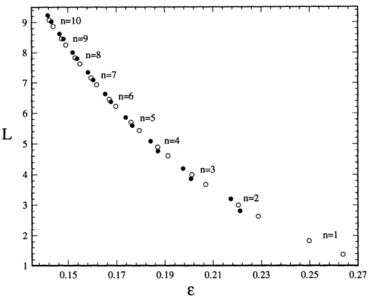
2-1. First few eigenvalues E and corresponding hump spacings L of three-hump bound states.

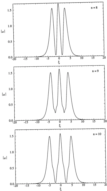
2-2. Numerically computed profiles of three-hump bound states for n = 2, 3, 4

and phase shift 0 = 7r/3.

2-3. Eigenvalues c and corresponding hump spacings L1 and L2 of four-hump

bound states for m = 1 and 8 < n < 20.

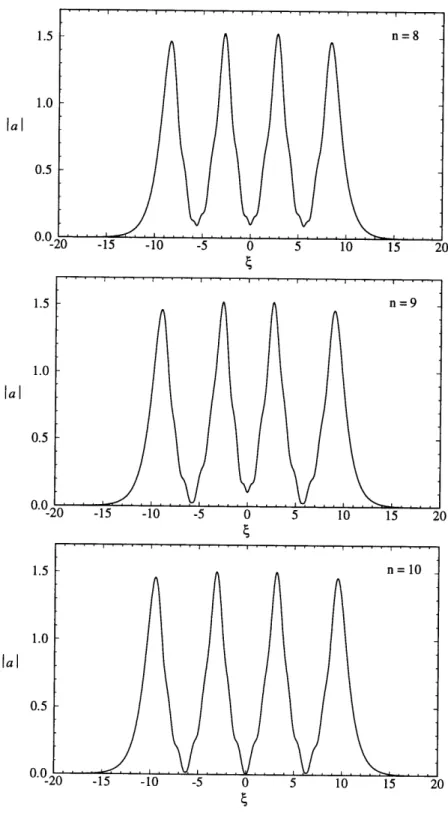
2-4. Numerically computed profiles of four-hump bound states for m = 1 and

n = 8, 9, 10.

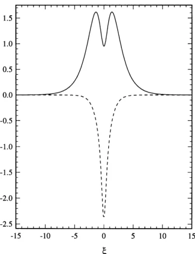
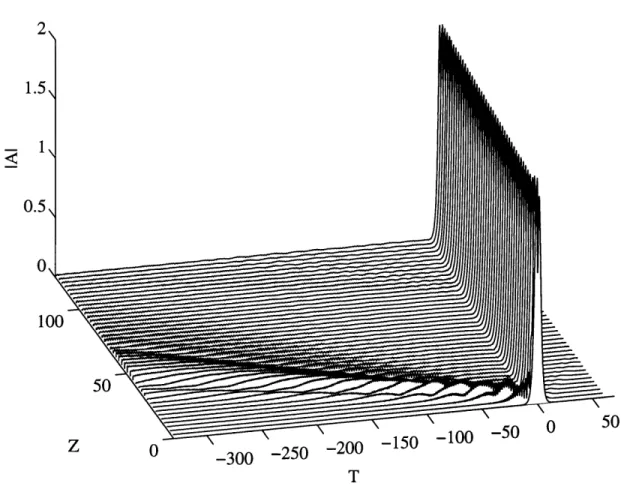
3-1. Fundamental bound state amplitude lal and instantaneous frequency O9. 3-2. Evolution of an infinitesimal initial disturbance to the fundamental bound

state.

3-3. Amplitude of trapped mode of fundamental bound state.

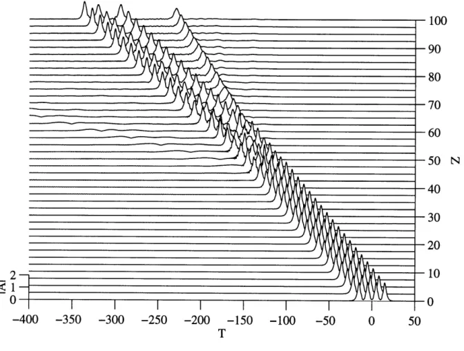
3-4. Evolution of a three-hump bound state A = 2.735.

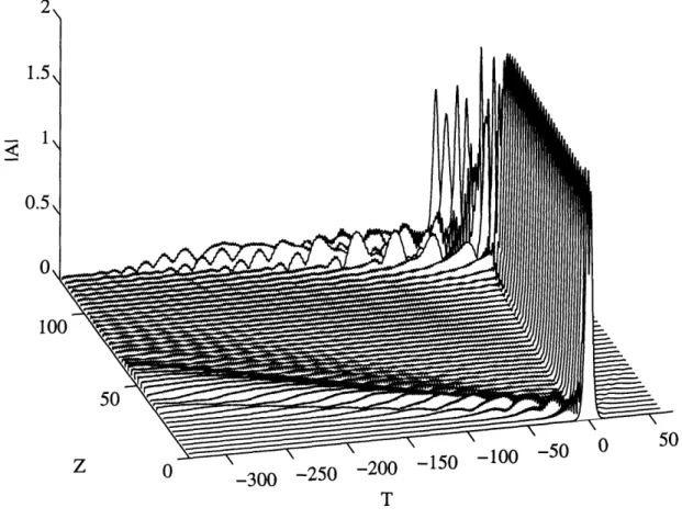
3-5. Evolution of a four-hump bound state A = 3.178.

3-6. Evolution of the fundamental bound state under a Gaussian disturbance at

Z = 0 with amplitude 0.14.

3-7. Evolution of the fundamental bound state under a Gaussian disturbance at

Z = 0 with amplitude of 0.15.

3-8. Comparison of perturbed and unperturbed bound state profiles at Z = 130

after a Gaussian initial disturbance of amplitude 0.14 at Z = 0.

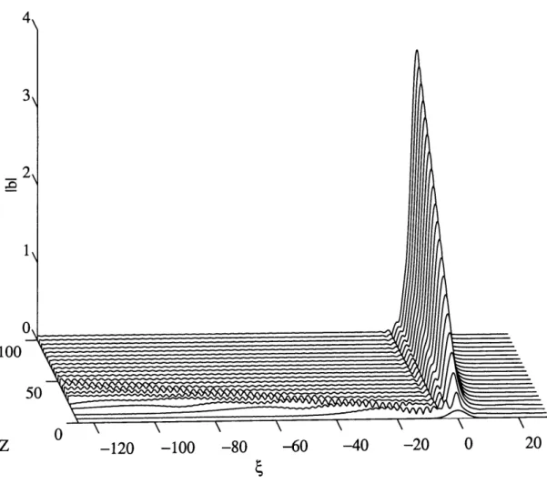
3-9. Evolution of the fundamental bound state under a frequency shift

3-10. Evolution of a pulse which at Z = 0 has a Gaussian amplitude profile and

phase close to that of the fundamental bound state. 48

3-11. History of numerical search for bound states using the continuation

CHAPTER 1

GENERAL INTRODUCTION

Over the past thirty years, substantial theoretical and experimental research on the interaction of high-amplitude electromagnetic waves with matter has resulted in the field now known as nonlinear optics. Recently, efforts have focused on investigating nonlinear optical phenomena specific to fiber-optic waveguides of the single-mode type used for the long distance transmission of pulses in modern optical communication systems. The bane of communication system engineers is dispersion-induced pulse broadening that results from higher-order dispersive effects that modify the group velocity of pulse envelopes (Agrawal, 1995). As the quest for high bit-rate communication systems demands the use of pulses of increasingly shorter width, pulse broadening effects become appreciable over shorter dis-tances necessitating the frequent use of costly repeater stations which reshape and amplify pulses preserving the signal integrity. To unleash the ultra-high speed performance of fu-ture optical communication systems in an economical way, the dispersion barrier has to be overcome.

A milestone in nonlinear fiber optics was reached in 1973 when A. Hasegawa proposed that a single-mode optical fiber could support solitons; nonlinear wave packets in which dispersive broadening effects are counterbalanced by nonlinear effects allowing propagation over long distances with little change in form. The concept was verified experimentally by Mollenauer et. al in 1980 with the advent of low-loss fiber and tunable laser sources. Using optical solitons, the bit-rate can be increased substantially while at the same time fewer and relatively cheaper repeater stations are needed.

Since then, research has focused on reducing the required power to launch a soliton which is inversely proportional to the square of the pulse width and directly proportional to the second-order fiber dispersion coefficient. A possible way of reducing the required power is to operate near the zero-dispersion wavelength (ZDW) in optical fibers, a point where the second-order fiber dispersion coefficient vanishes. Near the ZDW, the nonlinear

Schr6dinger (NLS) equation that describes the slowly-varying envelope of a nonlinear wave packet must be augmented by a third-order-derivative dispersive term in order to achieve a balance between leading order nonlinear and dispersive effects. The resulting modified nonlinear Schrodinger (MNLS) equation governs in general the propagation of nonlinear wave packets near a caustic of a dispersive wave system; a critical wavenumber where the linear dispersion relation has an inflection point.

In the context of wave envelopes in deep water it was shown by Akylas & Kung (1990) following a numerical procedure that the MNLS accepts steady pulse solutions in the form of two-hump bound states; wave profiles resembling a fusion of classical single-hump 'sech' profiles of the NLS. This result was also obtained using an asymptotic method by Klauder et. al (1993) who, in addition, reported that these pulses were highly unstable when third-order dispersion was strong.

Three main questions have remained open from these studies. As pointed out by Akylas & Kung, standard perturbation theory alone does not reveal that the MNLS accepts two-hump bound states. It was conjectured that the presence of exponentially small terms may be at the root of this, but this issue required further study. The analysis by Klauder et al. produced results in agreement with the work of Akylas & Kung but the details were so sketchy in Klauder's work that there was no general way of explaining the origin of the two-hump pulses or determining whether multi-two-hump pulses were possible. Asymptotic studies of the steady MNLS by several workers, notably Grimshaw (1995), used a perturbation analysis taking into account exponentially small terms to reveal that a single-hump solitary wave profile becomes nonlocal in the presence of third-order dispersion. Specifically, wave tails with non-zero amplitude at infinity appear and thus single-hump solitary waves of the steady MNLS cannot be locally confined pulses. This result is consistent with simulations of the time-dependent problem in which a single-hump wave begins to evolve towards a nonlocal state by radiating an oscillatory tail. Further analysis of the steady problem taking into account exponentially small terms is needed in order to explain how locally confined bound states can be formed by interacting nonlocal solitary waves.

substantiated, a systematic stability analysis was needed to assess the behavior of per-turbed bound states. Specifically, the results of a linear stability analysis combined with simulations of the full nonlinear pulse propagation problem would permit a more accurate assessment of stability.

Finally, it is well known that solitons of the NLS theory have the remarkably robust property that they can evolve out of general initial conditions which may be far from the exact 'sech' profile. As this property contributes to their usefulness in optical communi-cation systems, it is desirable to know whether bound states of the MNLS have a similar property.

These questions are addressed in this thesis using asymptotic and numerical meth-ods. The second chapter deals with the steady problem of determining pulse profiles of the MNLS. The asymptotic approach taken involves matching the tails of well-separated neighboring nonlocal solitary wave cores such that the composite wave is a locally confined solitary wave. The resulting multi-hump solitary waves are found to be in good agreement with numerical calculations. Although the analysis deals specifically with the MNLS, the asymptotic theory presented can be generally used to construct bound states of any system that accepts nonlocal solitary waves.

The third chapter investigates the stability of the steady bound states of the MNLS. Through a linear stability analysis and direct simulations of the MNLS it is found that the fundamental bound state may propagate stably for long distances in the absence of large perturbations. Results of simulations are used to predict the major challenges that might be faced in attempting to use these special pulses near the ZDW in an actual setting. It is hoped that this study may be useful as an aid to experimental researchers in nonlinear optics who may be interested in exploring the possibility of low power pulse propagation near the ZDW.

CHAPTER 2

FORMATION OF BOUND STATES BY INTERACTING NONLOCAL SOLITARY WAVES

2.1 Introduction

The term 'nonlocal solitary wave' has been used in recent years to denote a steady (or quasi-steady) disturbance that consists of a main core resembling a classical (locally confined) solitary wave and features oscillatory tails with non-zero amplitude at infinity. Nonlocal solitary waves arise in various physical settings (Boyd 1989), ranging from the transmission of nonlinear pulses in optical fibers (e.g., Wai et. al 1990, Karpman 1993) to the propagation of surface waves in a liquid layer (e.g., Vanden-Broeck 1991, Yang & Akylas 1996).

For a nonlocal solitary wave to be steady, the energy flux has to be constant throughout the disturbance and hence oscillatory tails must be present on both sides of the main core. On the other hand, for a nonlocal solitary wave evolving from a locally confined initial condition, an oscillatory tail is shed on one side only (dictated by the sign of the group velocity) so the disturbance is not entirely steady.

In this chapter, we shall focus on steady wave disturbances. Our goal is to construct multi-hump bound states, featuring more than one main core, by suitably piecing together nonlocal solitary waves. In prior analytical studies of this problem (Klauder et. al 1993, Buryak 1995, Grimshaw & Malomed 1993), bound states were approximated as a superposi-tion of nonlocal solitary waves, relying on a perturbasuperposi-tion procedure proposed by Gorshkov & Ostrovsky (1981) and Karpman & Solov'ev (1981) for weakly coupled solitary waves. While this approach has some intuitive appeal, it is not clear that it can be used when soli-tary waves have non-decaying oscillatory tails of exponentially small amplitude (Grimshaw

& Malomed 1993). Instead, following Yang & Akylas (1997), we seek steady bound states by matching both the oscillatory and the exponentially varying tail components of nonlo-cal solitary waves, ensuring that the energy flux remains constant throughout the entire disturbance.

This matching procedure is applied to the nonlinear Schrodinger (NLS) equation with a third-order-derivative dispersive perturbation. Among other applications, this perturbed NLS equation governs the propagation of pulses near the zero-dispersion wavelength (ZDW) in optical fibers. Here, locally confined bound states with no oscillations at their tails are possible, and families of such symmetric solutions with two, three and four main humps are constructed. The analytical results are confirmed numerically by a continuation procedure.

2.2 Nonlocal solitary waves of the perturbed NLS equation

Starting from Maxwell's equations, the complex envelope A of a weakly nonlinear pulse with carrier wavelength near the ZDW in a single-mode fiber can be shown to satisfy the perturbed NLS equation (Hasegawa 1989):

Ax + iPAtt + yAttt + iA2_{A* = 0, (2.1)}

where x denotes normalized distance along the fiber and t is a scaled time variable. The (real) constants 0 and y, respectively, control the relative significance of second-order and third-order dispersion: when the carrier wavelength coincides with the ZDW second-order

dispersion is absent and

3

third-order dispersive term becomes less important and (2.1) reduces to the classical NLS equation

which admits solitary-wave solutions in the anomalous dispersion regime (, > 0). Apart

from nonlinear optics, however, (2.1) governs in general the evolution of wavepackets near a 'caustic', where the group velocity is stationary and second-order dispersion vanishes

We seek permanent-wave solutions of (2.1) in the form

A = a(ý) exp(-iKx), (2.2)

where ( = t - vx and K allows for a possible wavenumber shift. Upon substitution into

(2.1), normalizing variables according to

1'1 5= ' ý' _(2.3)

and dropping the primes, it is found that a(() satisfies

aEC - a + a2a* + ic(vaC - ag) = 0, (2.4)

where

EV ,,K(2.5)

In terms of the parameter E, the NLS limit corresponds to E = 0, in which case (2.4)

has as a solution the familiar NLS solitary-wave profile:

a = 22 sech 5. (2.6)

On the other hand, equation (2.4) cannot be solved exactly for e

$

whether solitary waves are possible close to the ZDW. In an effort to answer this question, one may find corrections to the NLS solitary wave (2.6) by expanding a in powers of e. It

turns out (Akylas & Kung 1990) that v = 1 and

1 3 2 2

(_39

a = 2 S- 2 iESR + - E S+21S + (2.7)

42

4

2

with the notation S - sech (, R - tanh (.

It is interesting that, even though the perturbation expansion (2.7) can be carried to any order of E and every term remains locally confined, equation (2.4) in fact does not admit one-hump solitary-wave solutions that are locally confined. The reason is that oscillatory tails with exponentially small (in E) amplitude, beyond all orders of expansion (2.7), appear.

Several previous studies (Wai et. al 1990, Karpman 1993, Kuehl & Zhang 1990, Grimshaw 1995) have attempted to compute these tails using exponential asymptotics but the final results are not in complete agreement. Following a perturbation procedure in the frequency domain (Akylas & Yang 1995) (see Appendix A for details), we confirm the results obtained by Grimshaw (1995) through a nonlinear WKB technique in the complex plane.

Specifically, assuming that there are no oscillations at the left-hand tail, so that from (2.7)

a

-

--+ -0),

we find that an oscillatory component of exponentially small amplitude necessarily appears at the right-hand tail:

a -

+ 2i6

c00),

(2.8b)

where

6 = 22 7r- exp - (2.9)

E 2E

with C = 8.58. Apart from this asymmetric nonlocal solitary wave, there is also a

one-parameter family of symmetric (a(-() = a*

())

both tails:

a 2~ 2 iEeT-i 6 exp -i 4 iO) ( + oo), (2.10)

Cos 0

(_

where -7r/2 < 0 < r/2 is a phase-shift parameter that controls the oscillation amplitude. Our interest centers on steady wave profiles of the perturbed NLS equation in the form of locally confined bound states. Such disturbances, if they exist, have to be consistent with equation (2.4) which was obtained from (2.1) on the assumption of steady waves. In particular, it follows from (2.4), by multiplying with a* and extracting the imaginary part, that the flux

has to be constant. Furthermore, this invariant is equal to zero for a steady wave that is locally confined.

Hence, as noted by Grimshaw (1995), a nonlocal solitary wave with oscillations at one of its tails only cannot correspond to an entirely steady solution because according to (2.8)

Fi -+ 0 (( -+ -oo) while Fi - 462/E

#

solution as a quasi-steady solitary-like disturbance (evolving on an exponentially long time scale), its main core slowly decaying as it radiates an oscillatory tail. For the purpose of constructing steady bound states, however, we insist that the disturbance is steady and allow for a small exponentially growing component, consistent with the linearized version of (2.4), at the right-hand tail.

Specifically, we replace (2.8b) with

a - 2 e- Vi e e- + D e + 2i6 e-i/ (• - o).

The amplitude D = r ei€ _{is determined by requiring that the two invariants 7i1 and}

F2

_

(which follows from (2.4) by multiplying with a* and extracting the real part) vanish at

the right-hand tail (( -+ oc), as they do at the left-hand tail (( -+ -oo) where the wave is

locally confined according to (2.8a). These two constraints then yield to leading order

62 E

r =

I

= -7r+

,

and the asymptotic behavior of the right-hand tail is

2~2

C

CC -

eJ

i'

+

2i6 e-it/6

(( -+

00).

(2.13)

22

Note that the amplitude of the exponentially growing component of the tail is of higher order than the amplitude of the oscillatory part, and does not figure in the asymptotic analysis that determines the tail oscillations to leading order (see Appendix A). The expo-nentially growing part of the tail plays an important part, however, in matching the tails

of nonlocal solitary waves to construct locally confined bound states (see Section 2.3). In preparation for this matching, we next consider asymmetric steady nonlocal solitary waves with oscillatory and growing components at both their left-hand and right-hand tails. These waves can be deduced from the symmetric solitary-wave solution family (2.10) by super-posing an oscillatory component, exp(-i/ce), with complex amplitude proportional to 6. The resulting tails then can be expressed as

3i ; sin 0+ (

a 22 e2~ i eJ - 2i exp -i- - i_ ( -+ -oo), sin(9± + 0-)

3 3 sin 0

(

a 22 ~ e- + 2i sin(exp -i + (o-- 0),

in terms of the two phase parameters 0+ and 0_ (-7r/2 < 0± < r/2), the symmetric tails

(2.10) corresponding to the choice 0+ = 0_ = 0. Furthermore, we need to add exponentially

growing components to these tails so that the invariants (2.11) and (2.12) vanish and the nonlocal solitary wave can be part of a steady, locally confined bound state. Imposing these constraints one finds that

a - 22 e2~ - 1 sin2 + 2 e

7ie

2 sin2_{(9+ + 0_)}

(2

22 _(2.14a)

sin+ /) ( "•

)

(

- 2i _{sin(9 + 0)} sin(0+ exp -i- - iO_ _exp ( - -0o),

3 3

1

sin

8

₂

₁

a 22 e 2 e e- E

22 (2.14b)

sin_+ (

+ 2is exp

-i

(

sin(04 + 0_)

E

These are the most general expressions for the tails of a nonlocal solitary wave consis-tent with the requirement that it forms part of a steady, locally confined disturbance. In particular, expressions (2.8a) and (2.13), which are valid in the special case that oscillations

appear at the right-hand tail only, can be readily obtained from (2.14) by setting 0+ = 0.

Based on (2.14), we now proceed to construct locally confined bound states with more

than one main hump.

2.3 Locally confined bound states

The overall strategy for constructing multi-hump bound states involves piecing together nonlocal solitary waves such that their tails-both the oscillatory and the exponentially varying components-match smoothly.

2.3.1 Two-hump bound states

We begin with symmetric (about ( = 0) bound states having two main solitary-wave

humps centered at ( =

+L/2,

be present at the left-hand tail ( <« -L/2) of the hump centered at ( = -L/2. Hence,

setting 0+ = 0 in (2.14b), its right-hand tail is given by

a ~ e 2 e- 2 e - e -S -2 2 es e2

(2 E2 (2.15)

+2id exp -i ( + )/e]

(-L/2 <

< L/2),

where a is a phase constant to be determined. [If a(() is a solution of (2.4), so is a exp(ia).] Based on (2.15), symmetry of Re a about ( = 0 requires that

3 L 262 L

2ei cos (a- e) = e2 cos a+ ½)E (2.16a)

and

L -a= n + ) (n =0, 1, 2,..). (2.16b)

2E

From (2.16a), it follows that

a = - + - (2.17a)

2 2'

and

Conditions (2.16b) and (2.17) also ensure that Im a is antisymmetric about = 0 so0

a(-() = a*(() as required.

Recalling the definition of 6 in (2.9), condition (2.17b) relates the spacing of the two humps, L, to the dispersion parameter E:

L = - + 41n e - 2 n (2.18)

E 2

Combining (2.18) with (2.16b) then yields an equation that determines the specific values

of E = En (n = 0, 1,2,...) for which two-hump bound states are possible; correct to O(e),

2En(n + 1)7 = + 4 In En - 2 In (n = 0, 1,2,...). (2.19)

En 2

Equations (2.18) and (2.19) are consistent with the work of Klauder et. al (1993); the only

difference is in the value of the constant 7rC/2 = 13.4 which they approximated numerically

as 12.94.

The asymptotic expressions (2.18) and (2.19) are expected to be valid when en is small

(n > 1) so the two humps are well separated. Comparison with numerical results (Klauder

et. al 1993, Akylas & Kung 1990), however, indicates that (2.18), (2.19) provide a

reason-able approximation even for n = 0!

2.3.2 Three-hump bound states

We next proceed to construct symmetric bound states with three humps centered at

S= -L, 0, L. The middle hump is symmetric about ( = 0, and using (2.14a) with

0+= 0 = 0 the asymptotic behavior of its left-hand tail is found to be

a 2 aeZic eý 1 1 -2 1e-. E

-a ~

22

e2

e

-

e

8x/ý

(2.20)

-

Now, the left-hand tail of the middle hump must match smoothly with the right-hand tail of

and setting 0+ = 0 in (2.14b) the asymptotic behavior of its right-hand tail is

ei 2Cife - E2lif J e

a , ei a 2 e- i~i -L e -~ - 2 e ie L

Se22 e e

+ 2i exp [-i( + L)

(-L <

< -1),

where a! is a phase constant to be determined.

Matching of expressions (2.20) and (2.21) requires that

-8e - _e L exp i( + E eiE _{= -32 e- exp}

[i

i

[

For (2.22a) to be compatible with (2.22b), it is necessary that

cos 0 = 1_2' 62 = 8 2 e-L and a = Ir + c. Hence 0 = -7r/3 and

L = - + 4 In - 2 In

so the spacing of the humps of three-hump bound states as a function of e obeys the same relation (2.18) found for two-hump bound states. Furthermore, combining (2.23) with

(2.22c) and using (2.24), the values of c = en (n = 1,2,...) for which three-hump bound

states are possible satisfy the eigenvalue relation

E

(2n+

(2.22a)

(2.22c)

(2.23a)

I

Note that, for each n, _{the eigenvalues cn form pairs corresponding to the two values of}

0 = ± 7r/3. The asymptotic relations (2.24) and (2.25) will be compared against numerical

results in Section 2.4.

2.3.3 Four-hump bound states

Finally, we sketch the details of constructing symmetric bound states with four humps.

Taking the point of symmetry to be at ( = _{0 as before, the centers of the humps are}

placed at ( = ± L1/2 and at ( = ± (-L' + L2) = + L. It is then clear that, in addition

to imposing symmetry about ( = 0, we need to match the right-hand tail of the hump

centered at ý = _{-L with the left-hand tail of the hump centered at ( = -L 1/2 in the region}

-L

<<

•

-L

/2.

Specifically, making use of (2.14b) with 0+ = 0, the right-hand tail of the hump centered

at ( = -L is given by

a 2 e

ei 'l 2 Cli e-•i • e-e ee l i' eLze

226 2 _(2.26)

+

2i6 exp

[-i

_{(6 +}

L)

/E]

}

(-L

<<

_{<K -L}

_/2),

al being a phase constant. Similarly, using (2.14a), the left-hand tail of the hump centered

at ( = -L ₁/2 is given by

a

ei 2 {2• eie L1e /2 1 sin2 9+ 62 -- ie L1/2

e-Ssin

(

)

-

sin(

exp

[-i

+

+

0

(-L <

< -L1/2),

where a2 is another phase constant.

Matching of expressions (2.26) and (2.27) is achieved when

sin0+ = sin(O+ + 0_), (2.28a)

al + IE

=

a2 + ~E + 7r,

L2 = a1 - a2 + 0- + _{(2n - 1)7r}

f (n = 1, 2,...).

From (2.28a), one has

0+ =

_{2 2}

while (2.28b) gives

L2= -+ 4 In - 2 In (2.29b)

2

the same relation found earlier for two-hump and three-hump bound states (see (2.18) and (2.24)). Also, according to (2.28c), a1 - a2 = 7r + E, (2.29c) and (2.28d) becomes L2 = 2nxr + 0_ + E E (n = 1,2,...).

Next we impose symmetry about = 0. Using (2.14b), the right-hand tail of the hump0

centered at ( = -L 1/2 is given by

a eia2 e- e-L/2

sin _

+ 2i6 sin + exp

sin(04 + 0_)

2

_-

0)]

(-L1/2

<

<

This is symmetric about = 0 (a(-ý) 0 = a*(()) if

62 = 8 2 sin2(0+ + 0_) e-L 1 sin2 0_ a2 - •_ "-- = 2 i 2 - 2,E, L1

_{- = mr - -}

₊

a2 + 0+

2E

2

(2.31c)

Combining (2.31a) with (2.28b) and (2.29a) yields

= 4 sin2 0 2 exp(L2 - L1) (2.28c) (2.28d) (2.29d) < L1/2). (2.30) (2.32a)

Furthermore, according to (2.31b) a2 = (7r + e)/2, and, using (2.29a), (2.31c) becomes

L1 m + + 2 2 (m = 1,2, . (2.32b)

2E

2 2

2

Eliminating then L1 and L2 from conditions (2.29b), (2.29d) and (2.32), one is left with

two equations for 9_ and E:

7r 7rC

E(2nr + 0_ + +) = -- +41n - 2n (2.33a)

exp {[2(n - m) - 1]

ire

2

that determine the values of E = Emn (and the corresponding phase shifts 08_) for which

four-hump bound states are to be expected. The eigenvalues Emn now depend on two

integers, m and n, that control the hump spacings L1 and L2 through relations (2.32b) and

(2.29d), respectively. (In general, for symmetric bound states having 2N or 2N + 1 humps the eigenvalues depend on N independent integers.)

The analysis above of bound states with four humps is already typical of the general case where an arbitrary number of humps are pieced together, and we now turn to a comparison of the analytical predictions against numerical results.

2.4 Numerical results

In computing symmetric bound states of equation (2.4) numerically, we followed a shoot-ing procedure combined with continuation in the parameter E, as in Akylas and Kung (1990). Briefly, for a given value of e close to an analytically predicted eigenvalue, equation (2.4)

was integrated numerically towards the symmetry point ( = 0 starting at the right-hand

tail where the disturbance is known to decay exponentially:

Using as initial estimates the analytical predictions, the constants Ci and C2 were adjusted

by Newton iteration such that

Re aý = Ima = 0 (a = 0).

The exact eigenvalue was then determined by continuation in E so that the remaining

symmetry condition, Im aýE = 0, was also met at 6 = 0.

As mentioned earlier, detailed comparison between analytical and numerical results for two-hump bound states has been made elsewhere (Klauder et. al 1993); here we focus on three- and four-hump bound states. Figure 2.1 shows a comparison of numerically computed eigenvalues and corresponding hump spacings against the asymptotic results (2.24) and (2.25) for three-hump bound states. The agreement is generally good and, as expected, it improves for higher eigenvalues (increasing n) corresponding to bound states with larger hump spacing. It is worth noting that, for each n, there is indeed a pair of eigenvalues

depending on the choice of the phase shift 0 = ± 7r/3, consistent with (2.25). The two

lowest eigenvalues predicted by the analysis for n = 1 could not be located numerically,

however, suggesting that the eigenvalue relation (2.25) is not reliable for this low value of

n. Numerically computed profiles of three-hump bound states for n = 2, 3, 4 and 0 = 7/3 are displayed in Figure 2.2.

Turning next to four-hump bound states, recall that the eigenvalues emn depend on two integers, m and n, according to equations (2.33). For fixed m and n, these equations turn out to have multiple solutions (between 5 and 11 for 1 < m, n < 20). For reasons discussed

in Appendix B it was decided to fix m = 1 and search for the four-hump bound state

corresponding to the minimum eigenvalue for each value of n in the range 1 < n < 20. In

Figure 2.3, the hump spacings L1 and L2 are plotted against the corresponding eigenvalue

Emn together with the analytical predictions from equations (2.33), (2.32b) and (2.29d).

Again, the agreement between analytical and numerical results is quite good and becomes better as n is increased. For n < 7, on the other hand, the numerical procedure did not

9 8 7 6

L

5

1

FIGURE 2-1. First few eigenvalues e and corresponding hump spacings L of three-hump

bound states. (o): analytical results (2.24) and (2.25); (9): numerical results.

converge to a solution, suggesting that the bound state with the highest degree of

third-order dispersion (least eigenvalue) is the n = 0 two-hump wave for which E = 0.258 (Klauder

et. al 1993 , Akylas & Kung 1990). The numerically computed profiles of four-hump bound

states for m = 1 and n = 8, 9, 10 are displayed in Figure 2.4.

2.5. Discussion

We have developed an asymptotic theory for constructing steady multi-hump bound states of nonlinear wave systems that admit nonlocal solitary-wave solutions. The proposed technique is based on matching the oscillatory and exponentially varying tail components of steady nonlocal solitary waves, ensuring that the energy flux remains constant throughout

1 n=10 D n=9 - _o *0 - n=8 o n-=6 0 n=5 o nf=4₀ Sn=3 o * n=2 0 oo ' i nII , I l , ,I l i I , I .I . .l l ll.. . . I . .

FIGURE 2-2. Numerically and phase shift 0 = 7r/3.

computed profiles of three-hump bound states for n = 2, 3, 4

10 9 8 7 6 0.135 0.140 0.145 0.150 0.155 0.160 0.165 0.170 0.175 0.180

FIGURE 2-3. Eigenvalues E and corresonding hump spacings L1 and L2 of four-hump

bound states for m = 1 and 8 < n < 20. (o): analytical prediction for L1; (.):

computed value of L1; (A): analytical prediction for L2; (A): computed value of L2.

the disturbance. This approach seems more robust than superposition of nonlocal solitary waves used in previous work (Klauder et. al 1993, Buryak 1995, Grimshaw & Malomed

1993).

The asymptotic procedure has been applied to nonlocal solitary-wave solutions of the perturbed NLS equation. The NLS equation with a third-order-derivative dispersive per-turbation governs in general the propagation of wavepackets near a caustic, and, in the context of nonlinear optics, it is central to the transmission of pulses near the ZDW in optical fibers. Contrary to claims that there are no locally confined steady bound states of the perturbed NLS equation (Buryak 1995), we have explicitly constructed families of such bound states with two, three and four humps, and it is clear that states having an arbitrary number of humps are possible as conjectured by Klauder et. al (1993). The procedure has

n=20 n=18 n=16 o n=14 o n=12 0o o n=10 _0 n=8 0 . . .. . . 1 1[1 1 1 1 .I I I l l l I I I . ý .I I I I I I l l.

also been applied to construct bound states of the the fifth-order KdV equation (Calvo & Akylas 1997) in which nonlocal solitary waves also arise.

It is noteworthy that bound states of the perturbed NLS equation are eigensolutions since they occur at specific values of the parameter E defined in (2.5). In view of the scalings (2.2), (2.3) and (2.5), this implies that, for each eigenvalue E, there is a one-parameter solution family, and the envelope profile is completely determined when the carrier wavenumber is specified. This is in contrast to the usual NLS solitary waves which form a two-parameter family-both the carrier wavenumber and the peak amplitude can be specified arbitrarily-and raises the question of stability of bound states. As there are conflicting suggestions in the literature regarding this issue (Klauder et. al 1993, Buryak 1995), it will be considered in detail in Chapter 3.

lalI

lal

0.(

FIGURE 2-4. Numerically computed profiles of four-hump bound states for m = 1 and

n = 8, 9, 10.

4

CHAPTER 3

STABILITY OF BOUND STATES NEAR THE ZERO-DISPERSION WAVELENGTH IN OPTICAL FIBERS

3.1 Introduction

The propagation of weakly nonlinear pulses in optical fibers is governed by the non-linear SchrSdinger (NLS) equation which combines leading order dispersive and nonnon-linear effects. It is well known that the NLS equation accepts solitons with a single-hump sech profile if the carrier frequency of the pulse is in the anomalous dispersion regime of the fiber. The power required to generate a soliton is inversely proportional to the square of the pulse width and directly proportional to the strength of fiber dispersion. Early studies of optical solitons by Wai et. al (1987) focused on reducing the power by operating near the zero-dispersion wavelength (ZDW) in optical fibers; the borderline between normal and anomalous dispersion where dispersive effects are relatively weak. To describe propaga-tion near the ZDW, a third-order-derivative dispersive term must be included in the NLS equation resulting in a modified nonlinear Schrodinger (MNLS) equation. It is known from asymptotic studies (Grimshaw 1995) of the steady MNLS equation that the third-order term gives rise to nonlocal solitary waves; disturbances with a main core consisting of a classical solitary wave profile with non-decaying tails at infinity. In numerical studies of the time-dependent problem (Wai et. al 1986), the higher dispersion causes short-scale oscillations to radiate from a single-hump initial condition leading to a decay of the pulse amplitude. Because of a continuing interest in operating near the ZDW, recent studies have considered techniques of absorbing the radiation (Uzonov et. al 1995) while the objective of others (Buryak 1995) has been to search for special pulse structures that do not radiate when dispersive effects are weak.

equation does in fact accept locally confined symmetric pulses in the form of two-hump bound states; envelope profiles resembling a fusion of single-hump profiles of the NLS equa-tion. These solutions are possible for discrete values of a third-order dispersion parameter and are obtained in the case of anomalous dispersion. The asymptotic theory presented in Chapter 2 has shown that the MNLS equation accepts locally confined symmetric bound states featuring any number of humps greater than one; a result in agreement with numer-ical findings. In this chapter, we examine the stability of these steady solutions.

There are conflicting reports in the literature on the stability of bound states in general. Studies by Buryak (1995) and Buryak & Akhmediev (1994) of a fourth-order nonlinear Schrodinger equation address the stability question using variational methods to analyze weakly interacting solitary waves. Unfortunately, these methods cannot be applied to the important case of strongly interacting solitary waves and it is not entirely clear if these methods can be applied to the interaction of nonlocal solitary waves. As shown in Chapter 2, the construction of steady bound states cannot be completely explained as a suppression of radiation by superposing small amplitude periodic waves between solitary wave cores. Thus, it appears that the stability of bound states may depend greatly on nonlinear effects within the interacting regions between solitary waves. The stability of two-hump bound states of the MNLS equation has been discussed previously in the work of Klauder et al. (1993) where it was concluded that strongly interacting solitary waves are highly unstable. We reconsider this conclusion using linear stability analysis and direct simulation of the MNLS equation to show that strongly interacting solitary waves are in fact stable within certain limits. We also examine the effect of fiber loss, discuss the power requirements needed to establish these pulses, and simulate the propagation of approximate pulse profiles.

3.2 Steady bound states

governed by the MNLS equation (Agrawal 1995).

i kE k"' i n2 wo

Ez+

-

-E

= 0

2 6 caeff 2

where z denotes the propagation distance, t is the retarded time, n2 is the Kerr coefficient,

wo is the carrier frequency, c is the vacuum speed of light, aeff is the effective fiber core

area, and a is the fiber loss coefficient. The coefficients k0 and k.' are the second and third

derivatives of the carrier wavenumber evaluated at the carrier frequency.

It is convenient to non-dimensionalize this equation by introducing the following trans-formations:

T

-sg k

A

=

To E*

(3.2)

2

s gn k g6

(6To I

2

k'

2

Ikl1

where To is a characteristic pulse duration.

Substitution of (3.2) into (3.1) brings the MNLS equation to the following form:

Az + iPATT + ATTT + iA2_{A* + FA = 0. (3.3)}

The constant P controls the relative significance of second-order dispersion in the above

equation. Exactly at the ZDW, k0' vanishes and 0=0; while far from the ZDW (To0 kgl >

jkg•'),

[I1

For the determination of steady bound states we set 1=0 and consider the effects of loss in a later section. The bound states to be analyzed translate at a velocity relative to the reference frame moving at the group velocity at the carrier frequency. We assume a trans-lating duration coordinate and factor out possible frequency and wavenumber constants from the envelope. Accordingly, we introduce the transformation

A = a((, Z)exp[i(Qý - KZ)] (3.4a)

where v, K, and Q are constant parameters. Upon substitution of (3.4) into (3.3), it is found that a satisfies

-iaz + ,atK - Ka + a2_{a* + iat - iattt = 0 (3.5)}

where

S=

Q

It is convenient to normalize variables according to

-1 1

a

=IK a'

= |-'

Z =

II-Z'

(3.7)

and after dropping the primes, (3.5) becomes

-iaz + AaC - sa + a2a* + ivaý - iag = 0 (3.8)

where

A=

v

s = sgnK

(3.9)

Permanent form solutions of (3.8) are obtained by setting az = 0. Expressing the envelope

as a = r e'O the boundary condition

r

-4

0

(|0 -+

is imposed. Furthermore, with no loss of generality, the normalization

94 - 0 (|-| -

00)

is made.

From Akylas & Kung (1990) it was determined that solutions of (3.8) of the above form

are possible provided that v = 1 with sA > 0. As discussed in Chapter 2, solutions of

(3.8) are known in both numerical and asymptotic forms. Symmetric bound states can be obtained numerically by a shooting procedure combined with continuation. Details of this

procedure can be found in Akylas & Kung (1990). It is found that bound states are possible for eigenvalues An corresponding to different relative strengths of third-order dispersion.

Solitary waves of the NLS equation form a two-parameter solution family. Apart from translations in time and phase, a solitary wave of the NLS equation can be completely determined by fixing the peak amplitude and carrier frequency which may be specified independently. Solutions of the MNLS, on the other hand, form a one-parameter solution family as is clear from (3.6),(3.7), and (3.9). Once the carrier frequency is specified by fixing P and Q, the envelope profile and speed are completely determined. Solutions of the MNLS equation also differ from the NLS equation in that the instantaneous frequency distribution

Im{a }Re{a} - Im{a}Re{aC _(3.10)

varies throughout the wave profile. The two-hump bound state that will occupy most of

the discussion in this chapter corresponds to A = 2.4647 the profile of which is shown

in Figure 3.1. This value of A corresponds to the strongest third-order dispersion of any bound states found and also yields a relatively simple instantaneous frequency distribution in comparison to other multi-hump bound states. For the remainder of this study, this

pulse will be referred to as the fundamental with A = A0. Bound states obtained at larger

values of A, corresponding to weaker third-order-dispersion, feature humps that are spaced further apart and are weakly interacting solitary waves in this limit. In the calculations presented in this study, the bound states used will be the numerically determined steady solutions of (3.8) unless otherwise noted.

3.3 Stability of bound states

As a starting point, we examine the fundamental bound state when perturbed by in-finitesimal disturbances.

1.5 1.0 0.5 0.0 -0.5 -1.0 -1.5 -2.0 -2.5 -15 -10 -5 0 5 10 15

FIGURE 3-1. Fundamental bound state: amplitude

lal

3.3.1 Linear stability analysis

We consider small perturbations about the steady fundamental bound state,

a(6, Z) = ao( ) + b(6, Z) (3.11)

Substitution of (3.11) into (3.8) and retaining terms linear in b we obtain the disturbance equation:

It is useful to construct a conservation relation from (3.12) by multiplying the above equa-tion by b*, adding it to its complex conjugate and integrating:

d oo oo

d

if o(a*

_b*

dZ _mo

-oo

The above relation shows that the disturbance energy may grow by drawing energy from the steady state and serves as a check of the numerical procedure.

To investigate linear stability, two methods were used. For a given bound state corre-sponding to Ao, an initial Gaussian perturbation was tracked by solving (3.12) numerically. If the steady state is unstable, the energy of the perturbation grows indefinitely. A more general approach, however, is to use a modal decomposition of b and look for unstable

modes. The modal analysis begins by expressing the steady state as ao(O) = f(6) + ig(6)

and the perturbation as b(6, Z) = p(6, Z) + iq(6, Z).

Introducing this decomposition into (3.12), a system for p and q is obtained: 1

qz +

AoPýE

1o qý

Pz - Aoq0ý + q - (f2 + 3g2_{)q - 2fgp - - p6 + p~ = 0. (3.14b)}

We seek normal mode solutions of (3.14) in the form

{P} = {

)

and obtain the system

(a + 2fg)Q + AoPýý + (3f 2 ₊

2 1)P -

Qý

Qw

(a - 2fg)P -

AoQ0•

To determine the conditions for instability, we first examine the behavior of (3.16) far from the steady wave. In the limit IJI -- oo, (f, g) -- 0 and (3.16) reduces to

aP - AoQýý +

Q

-I

exp(K

(|( -+

oo)

(3.18)

the far-field dispersion relation is found to be

A O )(1Ao2) (3.19)

From (3.19) it is apparent that if n is pure imaginary then a must be pure imaginary

which implies that for an instability to be possible (Re a > 0), there must be a mode shape

that is trapped:

Q

The system (3.16) and boundary conditions (3.20) define an eigenvalue problem for the parameter a. For an eigenvalue a and mode shape (P((), Q(()), (3.17) also accepts

-a; (P(-0), -Q(-ý)) and hence the existence of a trapped mode is a sufficient condition

for instability. Because (3.17) also accepts a*; (P* (), Q* ()), the eigenvalue spectrum must

be symmetric about the Rea and Ima axes. We now turn to numerical results of the above two methods.

3.3.2 Numerical results

The possibility for instability was first explored by solving (3.12) numerically using a Gaussian initial conditions with the same full-width at half-maximum (FWHM) as the basic state being considered. To implement this solution, a split-step fourier spectral method was used. As a check of the numerical procedure, it was verified that the energy relation (3.13) was satisfied. As an additional check, computations were performed using a finite-difference method. There was negligible finite-difference between the results. The evolution of the disturbance corresponding to AX is shown in Figure 3.2. The solution indicates that

A

100

Z

-120

-100

-80

-60

-40

-20

0

20

FIGURE 3-2. Unstable evolution of an infinitesimal initial disturbance to the

funda-mental bound state.

part of the initial disturbance disperses away from the steady wave leaving a growing peak that eventually dominates the disturbance. To confirm the presence of instability, the modal analysis was implemented numerically using a 4th-order-accurate finite-difference method to discretize the system (3.16) subject to the boundary conditions (3.20). This results in a matrix eigenvalue problem

[C] {B} = a{B}. (3.21)

where the eigenvector {B} contains the mode shapes of P and Q corresponding to the

To improve the mode shape resolution and eigenvalue accuracy, the inverse power method with shifting was employed once an initial guess for the eigenvalues of interest had been obtained (see Appendix C for details).

The eigenvalue spectrum of the fundamental bound state consists of a number of periodic waves lying on the Im a axis and a pair of eigenvalues lying of the Re a axis corresponding to a trapped mode. The trapped mode of this bound state is shown in Figure 3.3 corresponding

to a growth rate of a = ±0.026. This instability is weakly trapped over a large extent

relative to the span of the steady wave and develops over a long propagation distance as

indicated by the small growth rate. This behavior is consistent with the roots K of (3.19)

when given the growth rate a. Specifically, there is a root corresponding to a short-scale

oscillation slowly decaying in ( < 0. As an additional check, the mode shape was used as

an initial condition to (3.12). The growth rate of energy agreed with that determined by modal analysis within 8% relative error. Based on this analysis, we conclude that if the two-hump bound state is slightly disturbed, the disturbance will begin to grow at a slow rate. This result raises the question of how nonlinearity will affect the disturbance and so we now turn to simulations of the MNLS.

3.4 Nonlinear evolution

As a starting point, we solve the MNLS equation (3.3) without loss given the unper-turbed initial conditions of typical two, three, and four-hump bound states existing in the presence of strong third-order-dispersion. In this case, the waves are perturbed only by the small truncation error. All calculations were performed using the symmetrized split-step

fourier method (Agrawal 1995) with a AZ = 5E - 4 and AT = 0.15 (see Appendix D for

details). A prominent feature of the MNLS equation is the possibility of a resonance of linear waves with the solitary wave. According to the linear dispersion relation of (3) the excited radiation propagates in the direction of T < 0. Thus, as the calculation proceeds

1.0 0.5 0.0 -0.5 -1.0 -40 -30 -20 -10 0 10 20

FIGURE 3-3. Trapped mode with growth rate a = 0.026: amplitude (P2 +Q2)2 ( ); real part P (- • -); imaginary part Q (- - -).

the -oo edge of the domain is closely monitored for incoming waves and the entire domain

is doubled to accommodate this radiation. As a check of the calculations, it was verified that the energy relation

S IAI2d<

=

-2Fr

I A2d<

(3.22)

dZ -oo

-oo

derived from (3.3) was satisfied. For convenience, the choice Q = 0 and K=1 was made

giving P = A in (3.9).

Using three- and four-hump bound states with moderate third-order-dispersion as initial conditions to the MNLS equation, it was observed that a break up of the pulse profiles into separate radiating pulses occurred at Z r 30 and 50 units, respectively as shown in Figures 3.4 and 3.5. In contrast, the two-hump bound state corresponding to Ao showed no sign of

-P ! ! I I I I i III |! II I i' I ...I l . I. I _Ii'I . . I I -Iii I Ii I IV I I II 1111111111111111111111'I I''''I''''I

2

1.5

1

0.5

0

50

40

30

20

10

0

-250

-200

-150

-100

-50

0

50

T

FIGURE 3-4. Evolution of a three-hump bound state A = 2.735 perturbed by only truncation error.

breakup at Z m 250. Simulations over longer distances (Z • 1000), after reducing the size of the solution domain, showed that only a small amount of radiation was being emitted in the direction of T < 0. Although the wave is linearly unstable, it appears that nonlinear effects provide a stabilizing action. This result differs from that presented in the work of Klauder et. al where it was reported that two-hump bound states with close hump spacings were unstable and rapidly destroyed by perturbations (truncation error, presumably). To clarify this further we now simulate propagation of the fundamental bound state when the initial conditions are altered by relatively large perturbations to magnitude and phase.

2

0

100

90

80

70

60

50 N

40

30

20

10

0

-400

-350

-300

-250

-200

-150

-100

-50

0

50

FIGURE 3-5. Evolution of a four-hump bound state A = 3.178 perturbed by only

truncation error.

3.4.1 Amplitude perturbations

Keeping the phase and hence the instantaneous frequency distribution constant, we add a Gaussian perturbation with the same FWHM as the unperturbed state. Solutions of the MNLS equation are shown in Figures 3.6 and 3.7 for perturbation amplitudes of 0.14 and 0.15, respectively. For clarity, only part of the solution domain is shown. In the first case, energy is radiated mostly in the direction of T < 0 over the first 15 units of Z. After 130 units of Z, the pulse amplitude shows an increase from 1.615 to 1.804 and the FWHM decreases from 6.454 to 5.993 as shown in Figure 3.8. The change in amplitude and width

1.5,

0.5,

1(

0

-300 -250 -UU

FIGURE 3-6. Evolution of the fundamental bound state under a Gaussian disturbance at Z=0 with amplitude of 0.14.

is in accordance with the scalings (3.7) derived in the analysis of steady bound states. Also, the wave speed and minimum instantaneous frequency evolve to values that are in excellent agreement with steady state values computed from (3.6),(3.9), and (3.10). It should also be noted that the instantaneous frequency shows a shift at the tails of the envelope from its initial value of zero. To explain the significance of this result, we note that after the pulse has evolved into this new state of higher amplitude and total energy the scalings indicate that /> p. By (3.4a), (3.5), and (3.6) it becomes apparent that if the amplitude is normalized such that instantaneous frequency is zero at the tails of the envelope, thereby

1.5, - 1,

0.5,

0,

-T

FIGURE 3-7. Evolution of the fundamental bound state under a Gaussian disturbance

at Z=0 with amplitude of 0.15.

absorbing the difference in frequency into the carrier frequency of the wave packet, then second-order dispersion becomes more dominant. Hence, the change in scale indicates a shift in the carrier frequency of the pulse away from the zero-dispersion wavelength. Also, this result has some intuitive appeal if we consider that a solitary wave of permanent form is the result of a balance between nonlinear and dispersive effects. The increase in amplitude should come with a commensurate increase in dispersion. As the disturbance amplitude is raised to 0.15, however, an instability develops that overtakes the pulse over a distance of 75-100 units of Z. Thus, the pulse shows conditional stability to perturbations of this type.

1.5

1A1 .0

0.5

0n

20 30 40 50 60 70

FIGURE 3-8. Comparison of profile at Z=130 (-) against unperturbed profile (- --)

of the fundamental bound state under a Gaussian initial disturbance at Z=0 with amplitude of 0.14.

3.4.2 Phase perturbations

As mentioned previously, unlike the single-hump pulse envelopes of the NLS equation, envelopes of the MNLS equation feature a variable frequency distribution or "chirp". Since this feature apparently keeps the two-pulses bound together, it is useful to know how sensitive the pulse structure is to variation in the instantaneous frequency. To examine this, we first consider a shift in frequency of the fundamental bound state by a factor Q':