Retrieving cloud, dust and ozone abundances in the Martian atmosphere using SPICAM/UV nadir spectra

(1)

HAL Id: insu-01512630

https://hal-insu.archives-ouvertes.fr/insu-01512630

Submitted on 29 May 2017

HAL is a multi-disciplinary open access

archive for the deposit and dissemination of

sci-entific research documents, whether they are

pub-lished or not. The documents may come from

teaching and research institutions in France or

abroad, or from public or private research centers.

L’archive ouverte pluridisciplinaire HAL, est

destinée au dépôt et à la diffusion de documents

scientifiques de niveau recherche, publiés ou non,

émanant des établissements d’enseignement et de

recherche français ou étrangers, des laboratoires

publics ou privés.

Martian atmosphere using SPICAM/UV nadir spectra

Y. Willame, A. C. Vandaele, C. Depiesse, Franck Lefèvre, V. Letocart, D.

Gillotay, Franck Montmessin

To cite this version:

Y. Willame, A. C. Vandaele, C. Depiesse, Franck Lefèvre, V. Letocart, et al.. Retrieving cloud, dust

and ozone abundances in the Martian atmosphere using SPICAM/UV nadir spectra. Planetary and

Space Science, Elsevier, 2017, 142, pp.9-25. �10.1016/j.pss.2017.04.011�. �insu-01512630�

(2)

Contents lists available atScienceDirect

Planetary and Space Science

journal homepage:www.elsevier.com/locate/pss

Retrieving cloud, dust and ozone abundances in the Martian atmosphere

using SPICAM/UV nadir spectra

Y. Willame

a,⁎

, A.C. Vandaele

a

, C. Depiesse

a

, F. Lefèvre

b

, V. Letocart

a

, D. Gillotay

a

, F. Montmessin

b

a_{Institut Royal d'Aéronomie Spatiale de Belgique, 3 av. circulaire, 1180 Bruxelles, Belgium} b_{Laboratoire Atmosphères Milieux Observations Spatiales, Paris, France}

A R T I C L E I N F O

Keywords: Mars atmosphere Nadir retrieval Cloud Dust Ozone SPICAM/UV

A B S T R A C T

We present the retrieval algorithm developed to analyse nadir spectra from SPICAM/UV aboard Mars-Express. The purpose is to retrieve simultaneously several parameters of the Martian atmosphere and surface: the dust optical depth, the ozone total column, the cloud opacity and the surface albedo. The retrieval code couples the use of an existing complete radiative transfer code, an inversion method and a cloud detection algorithm. We describe the working principle of our algorithm and the parametrisation used to model the required absorption, scattering and reflection processes of the solar UV radiation that occur in the Martian atmosphere and at its surface. The retrieval method has been applied on 4 Martian years of SPICAM/UV data to obtain climatologies of the different quantities under investigation. An overview of the climatology is given for each species showing their seasonal and spatial distributions. The results show a good qualitative agreement with previous observations. Quantitative comparisons of the retrieved dust optical depths indicate generally larger values than previous studies. Possible shortcomings in the dust modelling (altitude profile) have been identified and may be part of the reason for this difference. The ozone results are found to be influenced by the presence of clouds. Preliminary quantitative comparisons show that our retrieved ozone columns are consistent with other results when no ice clouds are present, and are larger for the cases with clouds at high latitude. Sensitivity tests have also been performed showing that the use of other a priori assumptions such as the altitude distribution or some scattering properties can have an important impact on the retrieval.

1. Introduction

The solar ultraviolet radiation can be used to study several key elements in the Martian atmosphere such as dust, ice clouds and ozone. Airborne dust is ubiquitous in the Martian atmosphere. It highly inﬂuences Martian climate due to its absorption of solar radiation, resulting in a local warming of the atmosphere. The monitoring of the dust cycle shows two main periods along the Martian year: the“cold” aphelion season where dust concentration is relatively low and usually very repeatable from one year to another (Smith, 2009); and the “warm” perihelion, where the dust loading is higher and characterised by frequent dust storms. These storms occur randomly in time with various size going from local storms to planetary events, inducing a larger variability during that period (Smith, 2008). Size, shape and scattering properties of Martian dust were studied using groundbased and remote observations (e.g.Tomasko et al., 1999; Clancy et al., 2003; Wolﬀ et al., 2009, 2010). Dust particles also serve as condensation nuclei for ice cloud formation.

Ice clouds play an important role in the Martian climate and are

related to the water vapour cycle. They were shown to induce an asymmetry in the transport of water vapour from one hemisphere to the other (Clancy et al., 1996). They usually appear under situation of adiabatically cooled upwardﬂows where the water vapour condenses on dust particles. The observation of clouds allowed to study their seasonal, spatial and even day-night distribution showing that clouds were observed under several forms: the equatorial cloud belt arising during cold aphelion (Smith, 2004, 2009), polar hoods that covers the poles of the winter hemisphere (Benson et al., 2010, 2011) and orographic clouds found above the tallest volcanoes (Benson et al., 2003, 2006). Ice clouds properties such as particle size and shape were also deduced from EPF observations, showing that there was two types of clouds (Clancy et al., 2003): type 1, which has a particle size of 1–2 µm, and is frequently observed in the southern hemisphere around aphelion but also above orographic heights and as altitude clouds; while type 2 has a 3–4 µm size and is observed in the aphelion cloud belt.

Ozone, which is an important UV absorber, is a very reactive species in the Martian atmosphere. It is produced through the photolysis of CO2

http://dx.doi.org/10.1016/j.pss.2017.04.011

Received 25 November 2016; Received in revised form 13 April 2017; Accepted 15 April 2017

⁎_{Corresponding author.}

E-mail address:yannick.willame@aeronomie.be(Y. Willame).

(3)

and O2that releases O atoms which recombine with O2to form the ozone molecule. The ozone abundance is anti-correlated with that of water vapour as the depletion of ozone is mainly due to the presence of odd hydrogen species HOxwhich are produced by the water vapour photo-dissociation (Lefèvre et al., 2004, 2008). Ozone is known to be present at high concentration from mid-to-high latitudes above the winter pole (up to 40 µm-atm), where the water vapour has condensed on the polar cap. The mid-to-high latitude ozone shows a large variability along the seasons as its quantities strongly decreases to 1–4 µm-atm during the summer (Perrier et al., 2006; Clancy et al., 2016). The high latitude ozone trapped in the polar vortex during winter, was recently shown to be a tracer to observe the dynamics of the vortex waves (Clancy et al., 2016). On the contrary, at low-to-mid latitude, the ozone concentration is more constant and remains in relatively low quantities: low quantities around 1 µm-atm are generally observed with noticeable increase up to 2–3 µm-atm around aphelion (Perrier et al., 2006; Clancy et al., 2016). That increase is related to the low altitude level of water vapour due to low temperature, allowing an altitude ozone layer to develop above 10–20 km (Lefèvre et al., 2004). Several instruments have been used to monitor one or more of these three species, among the most recent ones we find: MOC and TES aboard MGS; THEMIS on Mars Odyssey; OMEGA, PFS and SPICAM on Mars-Express; Pancam on the MER; and MCS, CRISM or MARCI from MRO. SPICAM is one of the instruments on board Mars-Express (MEX), orbiting around Mars since the very end of 2003. The SPICAM instrument is a spectrometer composed of two channels operating in the infrared and ultraviolet (UV) respectively. Works using SPICAM/UV have provided climatologies for the beginning of the mission: ozone for thefirst 1.2 Martian years (Perrier et al., 2006), and ice clouds for the first 2.2 MY (Mateshvili et al., 2007b, 2009).

In this paper, we present an improved retrieval algorithm developed to quantitatively analyse nadir spectra from SPICAM/UV. It allows to derive simultaneously the total abundance of ozone, dust and ice clouds as well as the surface albedo. The retrieval results can be used to analyse the spatial and seasonal distributions in order to contribute to complete our knowledge about these species and compare with the other existing climatologies. We start with a brief description of the SPICAM instrument and the data used in this work. We describe then the retrieval method that combines the use of the full radiative transfer code LIDORT (Spurr et al., 2001) and the optimal estimation method (Rodgers, 2000). The parametrisation chosen to model the atmosphere uses more recent results than in the previous works, based on SPICAM/ UV, ofPerrier et al. (2006),Mateshvili et al. (2007b)andMateshvili et al. (2009). We have performed the analysis of SPICAM/UV data on more than 4 MY and derived climatologies for the retrieved species. An overview of these climatologies is presented, describing the seasonal and spatial trends observed for each parameter. A comparison with climatologies obtained in previous studies is also provided. We also present the results of several sensitivity tests performed to quantify the impact of using diﬀerent assumptions as the altitude distribution or the scattering properties. We give a comparison between the retrieval results obtained by the present parametrisation and those obtained with the assumptions used in the previous SPICAM/UV works ofPerrier et al. (2006),Mateshvili et al. (2007b)andMateshvili et al. (2009).

2. SPICAM instrument and data

2.1. SPICAM instrument

In the present work, we used the measurements recorded in nadir viewing with the UV channel. SPICAM/UV covers the spectral range from about 118–320 nm with a resolution of 1.5 nm. The light is collected through a slit and recorded by a CCD detector. A measurement consists in 5“bands” (a band corresponds to the binning of 4 CCD lines) for which each line is composed of 384 illuminated spectral pixels of about 0.55 nm sampling. The nadir footprint of a 5 band scan usually

varies within 1–2 km along track and 2–15 km cross track. A detailed description of the SPICAM/UV instrument can be found inBertaux et al. (2006).

2.2. Data calibration

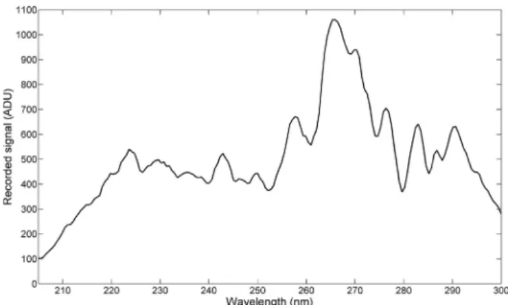
We have used level 1A data corrected for dark charge non uniformity and reading noise. The data are expressed in ADU (Analog to Digital Unit). An example of level 1A data is shown inFig. 1. The data are then converted into radiance factors (Rf): R λf( ) =πI λ F λ( )/S( ) whereλ is the wavelength, I is the scattered light intensity (radiance) entering the slit and FS is the solar irradiance at the top of the atmosphere (TOA). The solarﬂuxes used as references are based upon the public data of the SOLSTICE instrument on board the SORCE satellite.

We also applied a correction to take account of the dispersion of the incident light on the CCD. The method is based on the use of a Point Spreading Function (PSF) which is two dimensional Voigt proﬁle (for spatial and spectral dimension). It was calculated inMarcq et al. (2011)

using stellar observations. The Rf spectrum, corresponding to the measurement inFig. 1, is represented by the grey line inFig. 3.

2.3. Spectral interval

In order to save calculation time, the retrieval is performed on 8 different wavelengths in the 220–290 nm interval. The interval was chosen in order to work with the most reliable part of the spectra. Below 202 nm, the CO2absorbs (almost) completely the incident light. Between 202 and 220 nm, the calibrated Rfis not reproduced by the radiative transfer (RT) calculation. We suspect this discrepancy to be related to the calibration: the effective flux recorded becoming rela-tively weak makes these intervals more sensitive to inaccuracies in the calibration. Above 290 nm, the instrument sensitivity becomes weak (low values of the response curve) with a larger uncertainty and the calibrated Rfis also not correctly reproduced by the RT calculation (see

Fig. 3).

2.4. Binning and uncertainty

In order to increase the signal-to-noise ratio of the radiance factor, data binnings are performed, averaging on several measurements together and on several wavelengths: For the SPICAM data, we use the 5 bands of 9 consecutive measurements and a spectral binning on 9 wavelengths (≈ 5 nm); For the constructed solar spectrum FS, we use 7–8 consecutive daily SOLSTICE measurements (i.e. 4 FSper month) and a binning on the spectral interval equivalent to 9 SPICAM wavelengths.

Fig. 1. A typical level 1A nadir measurement in ADU from SPICAM/UV (Orbit 500, measurement 870).

(4)

The uncertainty on the radiance factor Rfis calculated from three contributions: 1) The uncertainty on the recorded ADUs which is composed of the shot noise and of the dark charge and electronic noise subtraction error; 2) The uncertainty on FS, calculated inMcClintock

et al. (2005), is approximately constant and always <3% in the 200–300 nm interval. In this work, we have used a constant value of 3%; And 3) the uncertainty on the instrument response curve provided by the SPICAM team (using v9 here).

The total uncertainty on the radiance factor in the 220–290 nm interval decreases from around 15–20% for a single band without binning to typically 2–4% when the binning is performed.

2.5. Measurement coverage

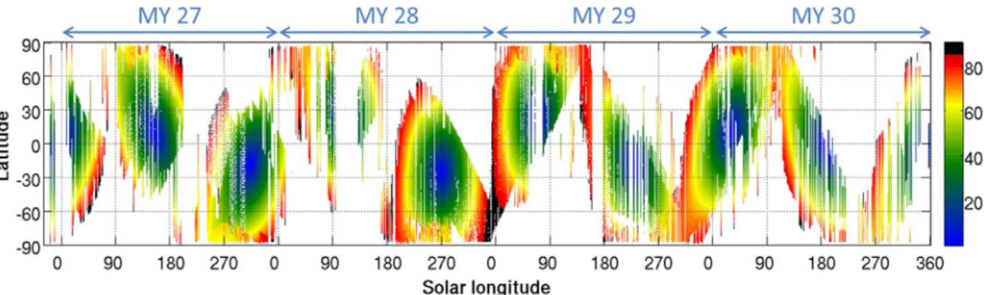
In this work, we analysed the 4ﬁrst Martian years of SPICAM/UV measurements, going from orbit 61 recorded atL =s 341° in MY26 to orbit 9821 taken at end of MY30 (using the arbitrary time reference deﬁned inClancy et al. (2000)). This corresponds to the period before September 2011 when MEX entered in Safe Mode 25 and which was followed by the steep increase of the number of defective spectra. The 4 MY period includes more than 2500 orbits in nadir mode, containing in total more than 4.5 million measurements. The seasonal coverage over the 4 Martian years is given inFig. 2.

3. Retrieval method

3.1. Retrieval algorithm overview

We describe here the retrieval algorithm which was developed to retrieve atmospheric and surface parameters from SPICAM/UV nadir measurements. The retrieval algorithm is an iterative process which consists in a main program which calls a sequence of diﬀerent subroutines: a cloud detection algorithm which was speciﬁcally devel-oped in order to identify in which measurements clouds have to be taken into account in the retrieval; a full radiative transfer (RT) model used for spectra simulation and for the calculation of the parameters’ derivatives; and an inversion method to estimate the best values of the retrieved parameters.

The goal is to deduce the ozone column, the dust and the cloud vertical opacities and the surface albedo from each single SPICAM measurement obtained in nadir geometry. As we retrieve column integrated quantities, the columns are obtained by scaling the a priori vertical profile. With the exception of ozone, these parameters corre-spond to broadband contributions to the radiance factor between 220 and 290 nm, which makes them difficult to decorrelate. We have decided after several tests to onlyfit 3 parameters simultaneously in order to keep them independent: ozone and dust are always retrieved while cloud isfitted if present, otherwise the surface albedo is the third retrieved parameter. An example of retrieval is shown inFig. 3.

The retrieval procedure is schematised inFig. 4and is summarised hereafter in several steps:

1. Cloud detection:

We start the procedure by applying the cloud detection routine which identiﬁes if the measurement is aﬀected by the presence of a cloud. Clouds appear bright in the UV compared to the dark regolith surface and asFig. 5shows, their presence results in a relatively large increase of the recorded signal. More precisely, the increase of signal is proportionally more important at longer wavelengths than at shorter wavelengths in the interval considered (220–290 nm). The principle of detection is based on the combination of two characteristics: a relatively large increase of the averaged signal (Sav) and an increase of a longer/shorter wavelength ratio (Rl s/).

This combination allows to differentiate from the effects due to dust, ozone and Rayleigh scattering. However, the surface reflection also shows such a combination. But as the regolith is strongly absorbing and partially occulted by the airborn dust layer, it induces only limited signal variations that can be differentiated by choosing an adapted (large enough) threshold. On the contrary, ice surface is very bright and can not be differentiated by such a threshold. Ice caps, based on the MCD (Mars Climate Database) v5.0 predictions, were therefore excluded in the cloud detection. An“uncertain” area of about 10° latitude is also delimited at the edge of the ice caps. The detections in these uncertain areas are treated by performing two

Fig. 2. Latitudinal coverage of SPICAM/UV nadir measurements during Martian years 27–30. The colour scale indicates the solar zenith angle (SZA) at the location and time of measurement. Values of SZA>85° were not considered in the retrievals and are black-coloured.

Fig. 3. Example of a spectral inversion performed with the algorithm developed (Orbit 500, measurement 870). The non-binned measured spectrum is represented by a grey line. The binned measured spectrum (MS) used for the retrieval is given in black dashed line with asterisk markers. The initial simulated spectrum (SS) obtained from the a priori conditions is represented in blue. The SS obtained after one iteration is given in magenta (RMS = 0.045). The SS obtained after a second iteration is represented in red and has converged (RMS = 0.014). An extended spectrum of iteration 2 is given in red dotted line, showing that the simulation can not reproduce the measurement outside the 220–290 nm range (cf.Section 2.3). (For interpretation of the references to color in thisﬁgure legend, the reader is referred to the web version of this article.)

(5)

independent retrievals: one including a cloud (above a regular surface) and a second considering ice surface (and no cloud). The solution with the bestﬁt is then selected.

Practically, each orbit is analysed separately. We simulate an averaged estimate signal Estav, analogous to Sav, using the a priori values. The idea being that Est ( )avim should follow the S ( )av im variations relatively closely for all im measurements wherein no cloud nor ice are present, while for the measurements aﬀected by the presence of clouds or ice, Savwould increase relatively to Estav. Estav is used to select the cloud- and ice-free (CIF) reference measurements (i.e. all the measurements for which Sav remains close or below to Estav). These CIF measurements are then used to build a CIF averaged signal Savref _{(and a CIF ratio Rl s}

/

ref_{) to which S}

av (Rl s/) is then compared in order to determine if the cloud detection

threshold tav(resp. tl s/) is exceeded. A cloud is thus detected when

both conditions are veriﬁed:

⎪ ⎪ ⎧ ⎨ ⎩ i i i i S ( ) > (1 + t )S ( ) R ( ) > (1 + t )R ( ) av m av av m l s m l s l s m ref / / ref/

where Savref_{(Rl s} /

ref_{) is obtained from S}

av(Rl s/) using a weighted average

on the nearest CIF measurements (the weight depends on the spatial proximity and surface elevation).

The cloud detection method will be described in more detail in a next paper dedicated to the results of our cloud retrieval with SPICAM (in preparation). It includes a comparison with the results obtained by OMEGA, another spectrometer on board MEX. 2. Creation of the a priori atmosphere:

The atmosphere is divided into 13 layers wherein we specify the characteristics and a priori quantities of each RT component. The thickness of the layers increases with altitude in order to partly compensate the decrease of density.

The a priori atmosphere come from the MCD v5.0, generated by the General Circulation Model (GCM) developed at LMD (Laboratoire de Météorologie Dynamique, Paris, France) byForget et al. (1999). The MCD provides the vertical proﬁles of temperature, pressure and mixing ratios for gases (O3 and CO2) and dust. A cloud layer, capping the dust layer (Smith et al., 2013), is added in the system if detected by the cloud detection routine (step 1). The parameters used to model the atmosphere are described in more detail in next

Section 3.3.

Here ends the preparation part and is followed by the iterative part consisting in repeating step 3 (RT calculation) and 4 (inversion) until convergence (step 5) is achieved (with a maximum of 8 iterations).

3. Radiative transfer calculation:

To perform the RT calculation, we use LIDORT (Linearised Discrete Ordinate Radiative Transfer,Spurr et al. (2001);Spurr (2002);Spurr (2004)), a RT code based on the discrete ordinate method (Chandrasekhar, 1960). LIDORT can generate radiances in a plane-parallel multi-layer atmosphere. It includes a pseudo-spheri-cal correction for the treatment of the solar beam attenuation and takes into account multiple scattering occurring in the atmosphere. The treatment of surface reﬂection is also included.

The v3.3 of LIDORT was adapted to our needs. We use it to simulate the spectrum using the built atmosphere and the varying retrieval parameters. It also calculates the spectrum analytical derivatives

Fig. 4. Schematic of the retrieval procedure.

(6)

associated to the retrieval parameters that are necessary for the inversion.

4. Inversion:

We have implemented the optimal estimation method (OEM) of

Rodgers (2000). It calculates a new set of values for the retrieval parameters in order to produce a new simulated spectrum (SS) that will converge toward the measured spectrum (MS).

The new set of parameters’ values is linearly extrapolated from the current set using: the analytical derivatives (calculated at step 3); the residue between the current SS and the MS (= SS-MS); the measurement error; and the a priori value of each parameter (for which we have to specify its variance to represent how much the parameter may vary around the a priori value). More details about the OEM implementation is given inSection 3.2.

5. Convergence test:

This routine verifies if the retrieval procedure has converged. There are two possibilities of convergence. Thefirst and ideal case is when the SSfits enough to the MS. To estimate the fit quality, we use a relative residue: (SS-MS)/DMS. DMS is the dataset mean spectrum which represents the average over all spectra of all orbits of whole the dataset. The convergence is reached when the root mean square (RMS) of the relative residue is minimised i.e. when it becomes lower than a defined convergence criterion ϵ. The RMS is calculated as: ⎛ ⎝ ⎜ ⎞ ⎠ ⎟

∑

N λ λ λ RMS(SS − MS) = 1 SS( ) − MS( ) DMS( ) λ _λ 2 (1) where Nλandλ are respectively the number and index of spectral pixels considered. The convergence criterion is calculated as the RMS of a 2% fraction of the DMS (ϵ = 0.02).

The other convergence criterion is when all the parameters’ values converge. It happens when the minimisation process reaches a minimum which implies that the residue and parameters only hardly vary between two consecutive iterations. We consider that the parameters have converged if they do not vary between two iterations by more than a deﬁned fraction (0.5%) relative to a reference value which corresponds generally for each parameter to a typical low-to-moderate value (regolith SSA: 0.07, ice albedo: 0.03, O3column: 5 µm-atm, dust OD: 0.5 and cloud OD: 0.2; a description of the parameters is provided inSection 3.3).

6. Saving results:

Once the convergence is achieved or after a maximum of 8 iteration loops, the procedure ends and saves the results. We keep the best set of parameters’ values, i.e. the set that gave the smallest RMS during the iterative procedure.

3.2. Implementation of the optimal estimation

The inversion of the parameters’ values from the observed spectra is performed using the optimal estimation method (Rodgers, 2000). The general equation of the radiative transfer forward model can be written as:

y=f x b( , ) + ϵ (2)

where y is the measurement vector (the measured radiance factor in this case), x is the true state vector (the parameters to be retrieved i.e. the ozone column, the dust and cloud opacities and the surface albedo) and b represents the additional parameters used by the forward model function f. The forward function f describes the complete physics of the measurement, including the description of the instrument. In the case of a moderately non-linear problem, the best estimatexof the solution of Eq.(2)is found by solving iteratively the equation:

xi+1=xa+Gi[( −y f x( )) +i K xi( i−xa)] (3) where the subscripts i andi + 1refers to the iteration loop number, xais the a priori of the state vector (i.e. the best knowledge of the parameters),

Ki is the jacobian matrix containing the derivatives of f relative to the parameters: K f x = ∂ ∂ i i (4)

These derivatives are provided by the RT model. We canﬁnally deﬁne the gain matrix Gi:

Gi= (Sa−1+K SiT·ϵ−1·Ki) ·−1K SiT· ϵ−1 (5)

whereSϵis the error covariance matrix of the measurements and Sais the a priori covariance matrix.Sϵis set to be diagonal and represents the error on

the radiance factor as described inSection 2.4. Saalso is set to be diagonal and represents the a priori parameters’ variance, i.e. one scalar for each parameter.

Inversion error. The error on the retrieved parameters is obtained from two contributions: the smoothing error (Ssmoo), which accounts for the sensitivity of the measurements/forward model to the variable to be retrieved (i.e. the measurement/forward model system does not allow perfectly reproducing the true atmosphere, but a smoothed value of it), and the error due to the measurement noise (Smeas). They can be expressed as:

Ssmoo= (A− )· ·(I Sa A− )I−1 (6)

Smeas=G S G· ·ϵ T (7)

where I is the identity matrix and A the averaging kernel matrix deﬁned by:   A x x x y y x G K = ∂ ∂ = ∂ ∂ ∂ ∂ = · (8)

We did not consider here the forward model error due to the additional parameters b and the error on the forward model itself. In that case, the total covariance error is given by the matrix S=Ssmoo+Smeasand can be rewritten as: S= (Sa +K Si · ·K) T i −1 ϵ−1 −1 (9)

Degree of freedom. As shown by Eq.(8), the averaging kernel matrix A represents the sensitivity of the retrieved parameters to the true parameters. We use the diagonal terms (Aii) to obtain informations whether the retrieved values of the parameters are extracted from the measurement or are rather coming from the a priori. These Aiiterms vary between 0 and 1 (as we consider only integrated columns) and are called degree of freedom (DoF): a DoF of 1 indicates that the retrieved value of the parameter was entirely deduced from the measurement while a DoF of 0 means that the retrieval was not sensitive in this parameter and the retrieved value comes therefore from the a priori. In the present case, there is one Aii corresponding to each parameter (thus 4 in total for: ozone, dust, cloud and surface reﬂectance). 3.3. Atmosphere parametrisation

We describe here the parameters used to model the interactions of the UV radiation with the atmosphere: the absorption by ozone molecules, the molecular “Rayleigh” scattering and the absorption and scattering induced by aerosols (dust and ice clouds). The inﬂuence of the diﬀerent parameters on a Rfspectrum is shown inFig. 5. 3.3.1. Ozone absorption

In the 220–290 nm range, the radiation is absorbed by Hartley band of ozone. That band is centred around 255 nm where absorption is the strongest. In this work, we have considered the recent cross-sections from the dataset ofGorshelev et al. (2014) andSerdyuchenko et al. (2014), which are in agreement with the results of the other previous works on ozone absorption of Brion et al. (1993)andMalicet et al. (1995). The uncertainty on the measurements is estimated to be within 2–3%.

(7)

The dataset contains eleven cross-sections measured at different temperatures extending from 193 K to 293 K by step of 10 K. However, the influence of temperature on the Hartley band is much weaker than in other spectral regions as explained inSerdyuchenko et al. (2014). As the temperatures at which ozone is retrieved usually vary between 150 K and 290 K, it implies that the difference with the cross-section temperature should not exceed 50 K. In our case, we estimate that the error on the cross-section due to appropriate temperature should therefore remain below 1% (based onSerdyuchenko et al. (2014)).

3.3.2. Rayleigh scattering

Rayleigh scattering is induced by the molecules in the atmosphere. The Rayleigh cross-section and phase function (PF) used in this work were calculated from several previous works considering an atmo-sphere made of 96% CO2, 2% N2and 2% Ar.

Theﬁnal Rayleigh cross-section was therefore obtained as follow:

σ= 0.96σCO2+ 0.02σN2+ 0.02σAr. For N2and Ar, we used the theoretical cross-sections calculated as in Sneep and Ubachs (2005) which both shows a very good agreement with their measurements (<1%, they worked between 470 and 570 nm). For CO2, as theory and measurements inSneep and Ubachs (2005)do not show such a good agreement, the cross-section was derived using aﬁt on the measurements in the UV from

Shemansky (1972),Karaiskou et al. (2004)1_and_{Ityaksov et al. (2008)}_.

Due to the wavelength dependence of the refractive index and the King factor, the expression giving the Rayleigh cross-section is not exactly proportional to the1/λ4_{law (where}_{λ is the radiation wavelength) and}

can be written as proposed inItyaksov et al. (2008): σR=σν4+ϵ, whereν

is the light wavenumber in cm−1. The parametersσandϵ were deduced by a linear ﬁt by taking the logarithm of the equation to obtain the following values: σ = 2.247 × 10−45_{and ϵ = 0.3801.}

The Rayleigh phase function p(cos ), whereθ θ is the scattering angle,

is decomposed in Legendre polynomials and requires two components: the zero order which coeﬃcient is always equal to unity (β = 10 ) and the

second order which coeﬃcient is related to the depolarisation ratio δ (β =2 δ_δ

1 −

2 + ). The depolarisation ratio used was obtained using the

individual depolarisation ratios of the three gases considered CO2, N2 and Ar. For N2and Ar, they were calculated as inSneep and Ubachs

(2005)and for CO2it was taken fromKaraiskou et al. (2004). Theﬁnal depolarisation ratio used to calculate the PF is δ ≈ 0.0777. The obtained Rayleigh scattering PF is shown in green inFig. 6.

3.3.3. Dust

Dust aerosols are responsible for absorbing and scattering the UV radiation. We consider the total vertical optical depth (OD) τd to quantify their extinction and the single scattering albedo (SSA) ω∼0to

represent the scattered fraction. In this work, we use the dust properties ofWolﬀ et al. (2010). For the SSA, we consider ω = 0.622∼0 at 258 nm

and ω = 0.648∼0 at 320 nm. The PFs come from T-matrix calculation

(Mishchenko et al., 1996) using a 1.5 µm cylindrical-shaped particles (Wolff et al., 2009) that was modified to agree with measurements as described in (Wolff et al., 2010): MRO/MARCI's EPF measurements were used to constrain and optimise the side-scattering (around 260 and 320 nm), while the back-scattering part was modified using the ground-based measurements from the Imager for Mars Pathfinder of

Tomasko et al. (1999)at 444 nm. These PFs are shown in Fig. 6and produce a predominantly forward scattering.

The SSA and PF used for the 220–290 nm interval in the present work were obtained by linear extrapolation of the 260 and 320 nm references.

3.3.4. Clouds

Water ice absorption coeﬃcient is very weak in the spectral region between 200 and 390 nm (Warren and Brandt, 2008). Ice cloud

absorption is therefore negligible and the single scattering albedo is set equal to unity ω = 1∼0 . The cloud opacityτcis thus entirely due to scattering. No wavelength dependence of the SSA is considered.

The PF used for ice clouds was provided by M.J. Wolﬀ (personal communication, Wolﬀ et al., in preparation). They used 3 µm ice particles size with a droxtal shape (Yang et al., 2003). No wavelength dependence was considered for the cloud phase function, which is shown onFig. 6.

3.4. Surface parametrisation

3.4.1. Regolith surface

To model the reflection of light on the Martian surface, we use the bidirectional reflectance of Hapke's theory (Hapke, 2005). We imple-mented the scenario case of the reflectance over large scale area of a rough surface. This formalism takes into account the opposition effect which induces a enhancement of back-scattering in the opposite direction to incident light.

The Hapke parametrisation used in this work for regolith surface comes from Wolff et al. (2014), which is in the continuity of the previous works ofWolff et al. (2009)andWolff et al. (2010)that used EPF (emission phase function) observations from respectively CRISM and MARCI on board MRO to derive the surface parameters (Hapke parameters were estimated for large areas in low dust loading condi-tions). The SSAω0used as a priori is location and wavelength dependent (extrapolated fromWolff et al. (2014), results) and varies between 0.05 and 0.11 (300 nm). The other parameters are kept constant: the opposition effect magnitude B = 1.00 ; the opposition effect width

h=0.06; the asymmetry parameter b=0.27, the forward scattering fraction c=0.30 and the macroscopic roughness θ = 20°.

3.4.2. Ice surface

The values of Lambertian albedo used to represent the reﬂection on ice polar caps were taken fromJames et al. (2005)which studied the southern polar cap with the High Resolution Camera on Hubble Space Telescope. They deduced values of the polar cap albedo from the visible down to the UV range.2

Fig. 6. Phase functions of the diﬀerent scattering processes considered in this work (μ= cosθ). The Rayleigh scattering that occurs on atmospheric molecules is approxi-mately isotropic (using a depolarisation ratio of 0.0777). The Mie scattering induced by larger dust and ice cloud particle is directed forward. However, clouds present a noticeable more important back-scattering probability than dust. For comparison, the dashed lines represent the Henyey-Greenstein (HG) phase functions with asymmetry parameter g=0.87 and g=0.70 as used inMateshvili et al. (2007a), (2007b). (For interpretation of the references to color in thisﬁgure legend, the reader is referred to the web version of this article.)

1_{The value at 206nm was not taken into account in the}_ﬁt.

2_{We have selected the results obtained for}_{“point 1” in}_{James et al. (2005)}_{which is}

considered as the more reliable due to known dust conditions measured nearby by MGS TES. We considered the average value of the three measurements at L =s 235°, 251° and

(8)

These results were obtained for a relatively high albedo region located on the seasonal polar cap made of CO2 ice (dry ice). Some deviations due to composition in the seasonal northern cap are possible, as well as seasonal variations and inter-annual variability (e.g. Hale et al., 2005; Langevin et al., 2007; Byrne et al., 2008) and also lowering of the reﬂectivity due to dust settling (e.g. Kieﬀer, 1990; Hansen, 1999)). As a priori, we considered an albedo value of 0.20 at 330 nm, a compromise between the values inJames et al. (2005)and the dark dust albedo. The wavelength dependence was obtained by a linear extrapolation of the values at 250 and 330 nm fromJames et al. (2005).

4. Examples of output climatologies

In this section, we show and discuss the climatologies obtained with the retrieval model using the nadir SPICAM/UV measurements of more than 4 Martian years (from MY 26.9 to 31.0). To produce these climatologies we used an exclusion criterion on the degree of freedom (DoF) of each parameter. Only retrieved parameters with a DoF >0.4 were kept to ensure that the retrieved value does not come only from the a priori. Another selection criterion is used on the retrieval residue to include only the retrievals that have a RMS < 0.04.3The seasonal distributions of the 3 retrieved atmospheric species, i.e. cloud OD, dust OD and ozone, are shown inFig. 7.

4.1. Clouds

4.1.1. Climatology overview

The top panel ofFig. 7 represents the seasonal evolution of the cloudiness. The two principal cloud features, the aphelion cloud belt (ACB) and the polar hoods, are both clearly observed. These water ice clouds are known to be repeatable from year to year (Smith, 2004, 2008). The results of the 4 MY analysis are combined inFig. 8 for a more visual overview of these cloud features.

The ACB occurs every year at low latitudes during the aphelion season (Smith, 2004, 2009). Its diﬀerent stages are well visible inFig. 8: the formation starts around L = 20 − 30°s , it shows a maximum extension and intensity between L = 80°s and L = 140°s and quickly disappears after. At its maximum of activity, the ACB completely encircles the planet at the Equator as shown inFig. 9top left. Around perihelion, (almost) no equatorial clouds are observed (cf.Fig. 9top right), except over Arsia Mons (clouds over volcanoes is discussed further). From the inter-annual point of view, we can see parts of the ACB stages in each MY inFig. 7top, depending on the coverage. The main changes from one year to the other are generally related to dust storms: As for example in MY27 where the cloud belt stops abruptly earlier in the season than usual (aroundL =s 135°) due to the rise of a local dust storm event (cf.Fig. 7middle), and which was also observed by THEMIS (Smith, 2009).

The polar hoods is known to occur above the polar regions of the winter hemisphere (Benson et al., 2010, 2011). Parts of their edges can be seen inFig. 7. The start of the northern polar hood (NPH) is well visible between L = 160°s and L = 200°s of MY27. We can see from the bottom panel ofFig. 9that the hood covers all longitudes, in agreement

Fig. 7. Seasonal evolution of the zonally averaged cloud opacity (top), dust opacity (middle, normalised at 6.1 mbar) and ozone column inμm-atm (bottom). The map covers the period going from late MY26 to the end of MY30, using a 2° × 2° grid. The white areas correspond to regions where no measurements were performed, the grey background represents the measurement coverage and the colour scale ranging from black to purple indicates the retrieved quantities.

3_{The maps provided in the following were obtained by satisfying the criterion for (at}

least) one of the two RMS calculations given hereafter: the RMS as described in Eq.(1)of

Section 3.1; and a modified RMS where the “DMS” (data mean spectrum) of Eq.(1)is replaced by the measured spectrum (MS). This modified RMS was set as we remarked that the criterion on only the first RMS was sometimes to restrictive for high signal measurements by rejecting somefit that we consider acceptable.

(9)

with MRO/MCS (Benson et al., 2011) which showed that NPH was forming a cloud cap above the pole. The edge of the NPH has also been observed around L = 240°s during MY28 and betweenL =s 330–350° in MYs 27 and 29. The southern polar hood (SPH) is also observed: Parts of the SPH edges are observed in the four MYs between L =s 0–60° (identiﬁed as SPH “phase 1” inBenson et al. (2010)) and between

L =s 120–200° during the MYs 27 and 29 (identiﬁed as SPH “phase 2” in

Benson et al. (2010)).

The tall volcanoes are particularly favourable for cloud formation.

Orographic clouds form because of adiabatic cooling that occurs with upslope winds arising on these volcanoes (Hartmann (1978)). Ice clouds are often observed above or near these volcanoes (Benson et al., 2003, 2006), with some example visible inFig. 9: On the top left panel, we observe that the highest retrieved opacities observed during the ACB maximum activity, are located over the large elevated Tharsis plateau, Olympus Mons [18 °S − 134 °W] and Elysium Mons [25°S–147°E]; On the top right panel, we notice that the only cloud retrieved around perihelion is located above Arsia Mons [10°S–120°W]

Fig. 8. Seasonal evolution of the zonally averaged cloud opacity. The values are averaged on the four Martian years of the dataset (from MY: 26.9 to 31.0).

Fig. 9. Example of spatial distribution of cloud OD for tree diﬀerent periods. On the top left panel, period L = 65 − 150°s (MY27-30), the ACB is clearly visible encircling the whole planet

at low latitude. The top right panel, period L = 200 − 300°s (MY27-30), corresponds to the cloud free season where (almost) no cloud were retrieved except above Arsia Mons

[10°S–120°W]. The bottom panel highlights the NPH observed between L = 160 − 200°s of MY27. The maps are averaged on a 2° × 2° grid using the same colour scale. Darkened pixels

(10)

which is known to be covered by clouds for the major part of the year (Benson et al., 2006).

A detailed analysis is left for a future paper (in preparation) dedicated to our ice cloud retrievals. The paper will provide compar-isons with results from other works using: MGS/TES (Smith, 2004), Mars Odyssey/THEMIS (Smith, 2009), MEX/SPICAM (Mateshvili et al., 2009) and MEX/OMEGA (Madeleine et al., 2012) concerning equatorial clouds; MRO/MCS (Benson et al., 2010, 2011) for the polar hoods; MGS/MOC (Benson et al., 2003, 2006) for the cloud presence above volcanoes.

4.1.2. Degree of freedom, error and uncertainty

The DoF for the retrieved cloud optical depth (COD) is larger than 0.9, implying that the retrieved values come from the measurements. The retrieval error on CODτclies generally between σ = 0.005 − 0.025c , increasing with cloud thickness. The relative error decreases as clouds are thicker and is summarised inTable 1.

However, this error does not include the uncertainty associated to the assumptions such as the cloud altitude or the scattering PF for which we have performed sensitivity studies on 7 orbits. It shows that the cloud PF has a strong inﬂuence on the retrieved COD. We compared the results obtained with the PF used in previous SPICAM/UV works of

Mateshvili et al. (2007b), Mateshvili et al. (2009) (using the value g=0.70) to these obtained with the nominal PF, both represented in

Fig. 6).Fig. 10 shows COD variations up to 400% and the diﬀerent

colours emphasise that the variations strongly depend on the phase angle: variations are the largest at low phase angle, decrease as the phase angle increases and become negative for phase angle>70°. Such a trend is expected when comparing the back-scattering tail of the PFs. From the convergence point of view, we observe only a little impact on the RMS (generallyΔRMS < ± 0.001).

The inﬂuence of the cloud altitude appeared to be less important. We tested low altitude cloud around 10–15 km (typical for ACBSmith et al. (2013) and used nominally in this work) compared to more elevated clouds (35 km, typical for polar hoods Benson et al. (2010),

Benson et al. (2011)):Fig. 11shows that the COD decreases between 0–4% when SZA is not too high (<65°). For these cases, a minor impact on the RMS is observed (ΔRMS < ± 0.001). Several higher COD variations (5–70%) are observed and correspond to cases with higher SZAs (>65°). These cases are also characterised by less good conver-gence of theﬁt with a decrease of the RMS (ΔRMS >0.005). The impact of the altitude of clouds seems therefore limited at low and mid SZA but can become important at high SZA, which has probably an impact on the polar hoods.

4.2. Dust

The middle panel ofFig. 7represents the seasonal evolution of the dust opacity. We noticeﬁrst that the expected dust loading diﬀerence between “clear” aphelion season and “dusty” perihelion season is clearly visible (e.g.Smith, 2004, 2009): the dust OD being lower and relatively constant around aphelion while it is larger and more variable during perihelion. This can also be seen inMontabone et al. (2015), hereafter abbreviated “MON15”, that used assimilation of the TES, THEMIS and MCS data to produce dust climatology between MY24-31. A second noticeable detail is the presence of important gaps during the

perihelion season that actually correspond to dust storm events and for which our retrievals have not converged (this will be discussed further in the text).

During aphelion, we can clearly distinguish the low dust OD patterns associated to the presence of the aphelion cloud belt, high-lighting the anti-correlation between dust and clouds: the dust optical depth reaches a minimum when the ACB is present at low latitudes between L =s 70–140°. Outside the ACB and the polar caps, the dust opacity is relatively constant beforeL =s 140°. Yet, some exceptions of higher opacities are observed: Several yellow spots are found at high latitudes in the northern hemisphere, especially during MY 29 and 30 afterL =s 90°, which are probably due to local dust storms that are likely to occur in the vicinity of the polar cap (Cantor et al., 2001). Another DOD increase is observed at low latitude aroundL =s 55° of MY 30, it is possibly related to a storm located on the Tharsis bulge between [110–70°W], but is not conﬁrmed by MON15. Another exception that worth to be highlighted is the dust increase aroundL =s 135° at low latitudes in MY27. The cause of this increase is a dust storm that arose a little earlier than usual in the aphelion season. This storm was also observed by THEMIS (Smith, 2009) and by both MERs (Smith et al., 2006). This was already mentioned in the cloud section as it is the reason for the early disappearance of the ACB. Another special case is the strong increase observed betweenL =s 145-155° of MY29 around 30°N. An increase of the dust activity is also visible in MON15 below mid latitudes at that corresponding period. The MER Spirit also recorded a very narrow but intense peak aroundL =s 155° (visible in the upper plot Fig. 13), which is also captured by our retrievals: SPICAM measurements near4_{the Spirit site reveal indeed usual opacity}

atL =s 147° followed by a strong increase atL =s 153° and a return to nominal level atL =s 157°.

During perihelion, the dust loading signiﬁcantly increases and is known to have an important inter-annual variability due to dust storm activity (Smith, 2004, 2009). We observe this variability when compar-ing the patterns in the 4 MYs, as for example with the appearance of the ﬁrst storm: it appear around L =s 135° for MY27 while and around

L =s 155° for MY30. For MY28 and 29, the measurement coverage is not optimal betweenL =s 140°-180°, but storm are observed from aroundL =s

Table 1

Summary of the inversion error on cloud OD retrieval.

Conditions Error

τ ∼ 0.05c 15–20%

τ ∼ 0.1 − 0.2c ∼10%

τ ≥ 0.3c ∼5%

Fig. 10. Influence of the cloud phase function on the retrieved cloud opacity. The “y” axis shows the variation of retrieved COD when using the PF defined inMateshvili et al. (2007b),Mateshvili et al. (2009)(g=0.7) instead of the nominal PF. The“x” axis represents the retrieved COD (nominal). The different markers represent the orbits: 232 (crosses, L = 9°s ), 331 (squares, L = 24°s ), 380 (circles, L = 31°s ), 424 (+, L = 36°s ), 891

(dots, L = 94°s ), 1385 (diamonds, L = 160°s ) and 1479 (triangles, L = 174°s ). The colours

represent the phase angle range: phase ≤ 35° in blue, 35°< phase ≤ 70° in green and phase >70°in red. (For interpretation of the references to color in thisﬁgure legend, the reader is referred to the web version of this article.)

(11)

170° and L =s 145° respectively. The coordinates (Ls, Lat) of the first storms for the four MYs match well with those of MON15 climatology. As mentioned, we observe gaps during the perihelion season which correspond to the important increases of the dust loading due to the large storm events: for example, we observe a large gap in MY28 between L =s 270–320° when a thick dust layer was present in the atmosphere due to the global dust storm that occurred that year. These gaps are explained by the fact that our retrieval does not converge when the dust OD becomes very large. From Fig. 5, we can see that the presence of dust results in a decrease of the Rf. And as we will show later, our retrievalfinds larger DOD than other results in the UV–vi-sible, which could reflect possible shortcomings in the dust modelling (e.g. optical properties, altitude distribution). Our retrieval procedure seems to compensate this impact by using more dust than really present in order to lower the simulated spectrum and to match the measured one. When the dust loading becomes very large, the measured spectrum becomes very low and can not befitted by the simulated spectrum. The reason for this could be that above a certain thickness of the dust layer, the opacity has (almost) no more influence on the Rf. The simulated spectrum approaches the measured spectrum but is unable to lower enough to reach it, no matter how much dust is set. So actually, in these cases, very high dust ODs are retrieved by the inversion procedure which however never converges resulting in much larger RMS values. The “edges” of these storm events are visible and their retrieved opacities are often relatively large, suggesting a rise of dust OD.

Fig. 12 shows the dust climatology obtained when the convergence

criterion that has been signiﬁcantly relaxed, revealing the large DOD increases that can be used for an easier qualitative comparison with MON15. The comparison reveals a general qualitative agreement between the two datasets and the coordinates of the major storms match well.

Our results for dust OD show a qualitative agreement with previous works. However, the retrieved DODs are usually higher when compar-ing to other studies in the UV–visible such as the MER/Pancam results (Lemmon et al., 2015) or the results obtained by MRO/CRISM (from private communication with M.J. Wolﬀ, related toWolﬀ et al. (2009)).

Fig. 13shows the comparison with the results ofLemmon et al. (2015)

using the MER/Pancams: We notice that the SPICAM OD are always higher than those obtained from Spirit. The agreement is better with Opportunity for which the retrieved ODs sometimes similar, and always higher for the rest. It is however important to precise that the MER results give the total aerosol opacities (ice cloud + dust) while those of SPICAM are given separately (magenta and green markers) and should therefore be summed when clouds are present for an adequate comparison.

Different possible reasons could explain this discrepancy. 1) The altitude profile: we use modelled profiles from the MCD v5.0 (Madeleine et al., 2011) which differ from the profiles measured by MRO/MCS (Kleinböhl et al., 2009). MCS observes a maximum in altitude which is not reproduced in MCD profiles (Navarro et al., 2014). And as shown inFig. 14, an increase of the dust elevation results in a decrease of the retrieved DOD and also improves the convergence (i.e. lower the RMS) in the large opacity cases. This shows the altitude profile is therefore probably part of the solution; 2) the optical properties are derived from a unique particle size: the dust particle size is known to vary with season and with altitude (1–2.5 µmClancy et al. (2003)); These explanations are being investigated and will be improved in future versions of our retrieval routine.

An example of spatial distributions is given inFig. 15. It shows the expected anti-correlation between the retrieved dust OD and topogra-phy: higher optical depth are observed in the lowlands of the northern hemisphere, while the southern highland lies under a thinner dust aerosol layer. The deep Valles Marineris canyon and Hellas basin, where the dust ODs are higher, are also well contrasted with their surrounding highlands. While the minima in dust loading are well observed above the highest volcanoes (i.e. the three Tharsis volcanoes, Olympus Mons, Alba Patera and Elysium Mons).

The DoF for the dust OD (DOD) is larger than 0.8 when no clouds are present meaning that the retrieved values come from the measure-ment. It remains generally between 0.6 and 0.8 when clouds are present, indicating still a good sensitivity of DOD for these cases. The inversion error on the retrieved DODs varies generally between 10% and 40%, it decreases with increasing DOD and increases when clouds are present. The retrieval error is summarised inTable 2.

Fig. 11. Influence of the cloud altitude on the retrieved cloud opacity. The “y” axis shows the variation of retrieved COD when using an elevated cloud layer (35 km) instead of the nominal cloud altitude (∼10–15 km), using in both cases layers of 5 km thickness. The “x” axis represents the retrieved COD (nominal). The different markers represent the orbits (cf.Fig. 10). The colours represent the SZA range: SZA ≤ 50° in blue, 50°< SZA ≤ 65°in green and SZA >65° in red. (For interpretation of the references to color in this figure legend, the reader is referred to the web version of this article.)

Fig. 12. Seasonal evolution of the zonally averaged dust opacity. This map must not be considered as reliable as the RMS criterion used to produce it was largely relaxed (RMS ¡ 0.2) but is useful to give a qualitative intuition of the large dust loading events.

(12)

This error does not include the uncertainty associated to the assumptions i.e. the altitude distribution, the SSA or the PF for which we have performed some sensitivity studies. The influence of the altitude distribution was already highlighted in the case of the MY28 dust storm (cf.Fig. 14). We have also tested the impact of the use of a Conrath profile (Conrath, 1975) with parameter γ = 0.03 during the aphelion season (on the same seven orbits as inFig. 10). The Conrath profile goes higher than the MCD average profiles used nominally in this work. It induces a decrease of the retrieved DOD generally between 30% and 55% that has little impact on the convergence (|ΔRMS|< ± 0.001) but is however usually slightly better with the more elevated profile. Larger DOD variations (up to −80%) are yet observed when relatively thick clouds (τ ≥ 0.1c ) or ice surface are present and SZA is large (>60°). In these cases, the impact on the convergence is important with |ΔRMS|> ± 0.005for the largest DOD relative difference (but not particularly in favour of one of the two profiles). It shows that the altitude distribution has a significant influence on the retrieved DOD which decreases as the profile reaches higher altitudes.

The impact of the scattering properties were also tested, a sensitivity test was performed for two sets of SSA (ω0) taken from Wolﬀ et al.

(2010): we compared the nominal values used for the retrieval ω =0

0.622 − 0.648 to the values ω =0 0.630 − 0.653 (258–320 nm) which

corresponds to a 1.8 µm particle size. The test was performed for two periods: the period of MY28 dust storm and during MY27 aphelion period (same seven orbits as inFig. 10). For the storm period, the use of the second SSA set induces a 2–3% decrease on the retrieved DOD compared to the nominal one. While for the aphelion period, we observe usually a 1–6% increase of the retrieved DOD that seems inﬂuenced by the cloud presence: generally 2–4% with clouds and 3–6% without (seeFig. 16). The impact on the convergence remains limited with a |ΔRMS|< ± 0.001. The studies of Wolﬀ et al. (2010)

shows a good agreement about the derived SSA with other works in the UV (e.g.Mateshvili et al., 2007a) and the error onω0is estimated to be 0.022 at maximum. This suggests that the SSA is relatively well constrained implying that the uncertainty on the SSA should therefore have a relatively limited inﬂuence on the retrieved DOD.

The phase function has been also tested. We compared the retrieval results obtained with the dust PF used in previous works ofMateshvili et al. (2007a) to these obtained with the nominal PF (both PFs are

represented in Fig. 6): Fig. 17 shows variations between [−10%,

+80%] with the maximum decreasing from +80% at low DOD to +20% for the highest DODs. No clear trend related to phase angle is reported for the dust PF test (as it was the case for the cloud PF tests, cf.

Fig. 10). This reﬂects the fact that the direct back-scattering due to dust

is less important than it is with clouds, as it can be seen inFig. 6. However, the presence of clouds or ice surface seems to influence the DOD variations as illustratesFig. 17: the presence of cloud or ice is generally related to a larger variation than when none of them is present. The PF influences the retrieval convergence. The impact is generally limited with |ΔRMS|< ± 0.001 at low DOD (τ < 0.3d ); Im-portant RMS difference (|ΔRMS|>0.004) are frequently observed at high DOD (τ > 1.1d ); Between τ = 0.3 − 1.1d , limited impact is observed except for the cloudy cases (|ΔRMS|= 0.002 − 0.007) and for the cases of negative variations (|ΔRMS|= 0.001 − 0.003).

4.3. Ozone

The bottom panel ofFig. 7represents the seasonal evolution of the ozone total column. We notice that the expected seasonal trend of ozone, anti-correlated to water vapour (e.g. (Fedorova et al., 2006; Lefèvre et al., 2004)), is well observed: the largest ozone quantities are observed at high latitudes in the winter hemisphere where water vapour has condensed on the polar cap. While the ozone columns are much lower at low latitudes and in the summer hemisphere.

The winter poles are not probed by SPICAM/UV due to the absence of solar illumination during the polar night, but the increase of ozone column at the edge of the winter polar region is clearly visible. During the spring in the northern hemisphere, the SPICAM measurements extend almost up to the pole which allows to observe there the decay of the polar ozone. The retrieved column in this high abundance region generally ranges between 5 and 25 µm-atm.

Outside the winter polar regions, i.e. at low latitude and in the summer hemisphere, we observe low columns of ozone, remaining generally below 3 µm-atm. However, we notice two relatively signiﬁ-cant exceptions to this during the perihelion season (L = 180 − 360°s ) of MY28: theﬁrst is the increase that occurs at high latitudes between 70 and 80°S during the southern summer (L = 250 − 285°s ); the second is

Fig. 13. Dust opacity (300 nm) retrieved by our method compared to the values obtained with the Pancam instrument on board Spirit and Opportunity rovers. The Pancams provide measurement of aerosol optical depth at 440 nm (dark blue dots) and 880 nm (red line) through direct solar imaging. Spirit measurements are offset by 2. SPICAM results are those obtained in a 6° × 6° box centred on each rover's location and are given by“x” (for Opportunity's site) and “+” markers (for Spirit's site, offset by 2). The dust and cloud optical depth are represented in green and magenta respectively. The dust OD average on LΔs= 5°intervals are also given (black symbols). It is useful to precise that the dust opacities at 300 and 440 nm are more or less similar (according to T-Matrix calculation, the OD at 300 nm is about 2–3% lower than at 440 nm). The Pancam opacity plots are reproduced fromLemmon et al. (2015). (For interpretation of the references to color in thisfigure legend, the reader is referred to the web version of this article.)

(13)

observed around 30°N and L = 230°s . Both cases were found to be an artefact due to high dust opacity.5

Another noticeable feature is the increase of O3column that occurs at low latitudes between L = 45 − 100°s and which was observed in other previous works (Perrier et al., 2006; Clancy et al., 2016) and reproduced by the models as a relatively important ozone layer present in altitude, between 30 and 60 km (Lebonnois et al., 2006; Lefèvre et al., 2004, 2008).

The retrieved ozone column depends on the aerosol loading in the atmosphere (quantity and altitude proﬁle). As mentioned before, we

suspect to have shortcomings in our dust modelling which impacts the quantitative comparison with other results. However, some partial comparisons were performed to estimate the agreement with previous studies.

The comparison with MARCI results (Clancy et al., 2016) shows a qualitative agreement in the diﬀerent seasonal patterns mentioned above. On the quantitative point of view, comparing the seasonal distribution maps, SPICAM and MARCI seems in reasonable agreement: especially for the northern high latitude ozone between L =s 315–90° and the low latitude increase between L =s 45–100°. Higher values seems to be retrieve with SPICAM at the edge of the southern polar cap between L =s 0–210° and also for the northern high latitude ozone betweenL =s 150–200°. However, a more adequate quantitative analysis has to be performed as ozone variations can occur relatively quickly, especially at the pole where its distribution follows the polar vortex waves (Clancy et al., 2016). About hundred simultaneous and co-located SPICAM-MARCI measurements ( ± 3 h time and ± 1°lat-lon)

Fig. 14. Retrieved dust optical depth (left) and profile elevation in km (right) corresponding to the different a priori altitude profiles tested: (top) MCD climatological average profiles (MCD Scenario 1, used nominally in this work); (middle) MCD storm profiles (MCD Scenario 5); and (bottom) Conrath profile of parameter γ = 0.007. By dust elevation we mean the elevation at which the dust profile reaches 98% of its total OD (integrated from the ground). The altitude corresponds actually to the bottom altitude of the layer in which that condition is reached (the layers are 5 km thick from 10 to 40 km and 10 km thick at higher altitudes). The optical depth displayed is scaled at 6.1 mbar to remove the topography effect.

5_{It is obvious by visual check that the}_{ﬁt has not worked for these cases which spectra}

do not show the ozone signature. These spectra have been measured in relatively important dust loading and with a high solar zenith angles (>60°), which increase the airmass and the slant opacity of dust, reducing therefore the impact of ozone absorption in the spectra. Large ozone quantities were inadequately used here by the inversion to lower the signal and reduce the residual.

(14)

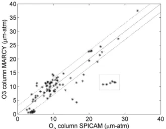
were identified (personal communication with T. Clancy). The compar-ison is given inFig. 18: it appears that SPICAM and MARCI follow the same trend for the 70–75°N results with deviation that usually remain within ± 3 μm-atm. While the results obtained at 33–36°S show a important difference with significantly larger SPICAM values.

The spatial distributions are also in qualitative agreement with MARCI's map: the correlation of ozone with topography is observed in our results with larger ozone columns found above area of lower elevation. We can clearly see onFig. 19that the high latitude winter ozone (with high abundances) follows the boundary between the northern lowlands and the southern highlands and higher columns are also observed in the deep basins (Hellas and Argyre) of the southern hemisphere.

A partial comparison with the work ofPerrier et al. (2006), which obtained thefirst ozone results with SPICAM, was also performed. The two sets also show a qualitative agreement of their seasonal trends, but some quantitative differences are reported. The main differences seems to occur when clouds are present and which were not taken into account inPerrier et al. (2006): For the large ozone columns observed at high latitude in the winter hemisphere, when no clouds are present, we generally observe an reasonable agreement between the retrieved

Fig. 15. Composite spatial distribution of the dust optical depth for the aphelion period (L =s 0–180°). The map is averaged on a 2° × 2° grid and was obtained for the complete dataset

(MY27-30). Darkened pixels indicates the measurement coverage and the colour scale ranging from dark blue to red corresponds to the retrieved dust opacity. No scaling was performed on the optical depths. (For interpretation of the references to color in thisﬁgure legend, the reader is referred to the web version of this article.)

Table 2

Summary of the inversion error on dust OD retrieval.

Conditions Error

In general ∼10%

– During ACB maximum 15–40%

– Above polar caps with low DOD

Thin clouds presence (τ ∼ 0.05c ) ∼15–20%

Fig. 16. Influence of the dust SSA on the retrieved dust opacity. The “y” axis shows the variation of retrieved DOD when using the SSA of the 1.8 µm particle size set instead of the nominal 1.6 µm set (both fromWolff et al. (2010)). The“x” axis represents the retrieved COD (nominal). The different markers represent the orbits (cf.Fig. 10). The colours represent the presence of ice surface or cloud: no cloud nor ice in blue, thin cloud (τ ≤ 0.1c ) in green, thick cloud (τ > 0.1c ) in red and ice in cyan. (For interpretation of the

references to color in thisﬁgure legend, the reader is referred to the web version of this article.)

Fig. 17. Inﬂuence of the dust phase function on the retrieved dust opacity. The “y” axis shows the variation of retrieved DOD when using the PF as inMateshvili et al. (2007a)

instead of the nominal PF (fromWolﬀ et al. (2010)). The“x” axis represents the retrieved COD (nominal). The diﬀerent markers represent the orbits (cf.Fig. 10). The colours represent the presence of ice surface or cloud: no cloud nor ice in blue, thin cloud (τ ≤ 0.1c ) in green, thick cloud (τ > 0.1c ) in red and ice in cyan. (For interpretation of the

references to color in thisﬁgure legend, the reader is referred to the web version of this article.)

(15)

ozone values of the two sets. On the contrary, when a cloud is present, we often notice a signiﬁcant increase (which can reach a factor 2) of our retrieved ozone values compared to those of the old set. Incidentally, the transition between the retrieval cases of an ice cloud above regolith and ice cap with no cloud is marked by a steep and discontinuous decrease of the ozone quantity an is shown inFig. 20. We will have to consider this issue to obtain a smoother transition by introducing a case in which both clouds and ice surface coexist.

If we consider the low latitude ozone (with low abundances), the results show generally a good agreement between the two sets and do not appear to be much aﬀected by the presence of clouds.

The DoF for the retrieved ozone column is usually larger than 0.8, meaning that the results come from the measurements. The retrieval error on the ozone total column varies generally depending on the season and location. The retrieval error is summarised inTable 3.

The error provided here does not take account of the uncertainties on the assumptions such as the altitude distribution. We have performed some sensitivity tests to estimate the impact of the altitude

distribution on the retrieved O3column: we have compared the use of MCD v5.0 ozone proﬁles (nominal in this work) with a constant volume mixing ratio (vmr) proﬁle, resulting in a O3column variation between [−40%,+30%] for low ozone quantities (<2 µm-atm) and a decrease between 10% and 60% for larger ozone column. From the convergence

Fig. 18. Comparison of the retrieved ozone column between MARCI and SPICAM. The comparison is made between simultaneous and co-located measurements ( ± 3 h time and ± 1° lat-lon). These measurements have been recorded between L = 0 − 90°s , and

almost all of them were located between 70 and 75°N except the 6 points surrounded by the dotted rectangle which were obtained between 33 and 36°S (around L = 45°s ). The

x=y line is also represented for an easier comparison.

Fig. 19. Spatial distribution of the ozone column (μm-atm) at the beginning of the aphelion period (L = 0 − 30°s ).

Fig. 20. Retrieved ozone column for several orbits between L = 0 − 30°s of MY27. Low

ozone quantities are observed at low latitude and start to increase at mid-latitude. towards the poles. The transition from ice cloud above a regolith surface to ice surface with no cloud is well visible and marked by a sharp and discontinue decrease, it occurs: around 64°N for orbit 231; after 58°N for orbit 285; and in the four orbits reaching the south pole (around 70°S, 65°S, 65°S and 53°S for orbits 302, 294,308 and 371 respectively).

Table 3

Summary of the inversion error on ozone column retrieval.

Conditions Error

Above polar caps ∼5%

(highest ozone columns)

Edges of the polar caps 10–20%

Outside polar region ∼100%

(very low ozone columns)

Low latitude between L = 30 − 100°s 30–60%