The MIT Faculty has made this article openly available. Please share how this access benefits you. Your story matters.
Citation Zymnis, D.M., A.J. Whittle, and I. Chatzigiannelis. “Effect of
Anisotropy in Ground Movements Caused by Tunnelling.” Geotechnique 63, no. 13 (October 1, 2013): 1083–1102.
As Published http://dx.doi.org/10.1680/geot.12.P.056
Publisher Thomas Telford Ltd.
Version Author's final manuscript
Citable link http://hdl.handle.net/1721.1/92766
Terms of Use Creative Commons Attribution-Noncommercial-Share Alike
EFFECT OF ANISOTROPY IN GROUND MOVEMENTS CAUSED BY TUNNELING by
Despina M. Zymnis1, Ioannis Chatzigiannelis2, and Andrew J. Whittle3
ABSTRACT
This paper presents closed-form analytical solutions for estimating far-field ground deformations caused by shallow tunneling in a linear elastic soil mass with cross-anisotropic stiffness properties. The solutions describe 2-D ground deformations for uniform convergence (uε) and ovalization (uδ) modes of a circular tunnel cavity, based on the complex formulation of planar elasticity and superposition of fundamental singularity solutions. The analyses are used to interpret measurements of ground deformations caused by open-face shield construction of a Jubilee Line Extension tunnel in London Clay at a well-instrumented site in St James Park. Anisotropic stiffness parameters are estimated from hollow cylinder tests on intact block samples of London Clay (from the Heathrow Airport Terminal 5 project) while the selection of the two input parameters is based on a least squares optimization using measurements of ground deformations. The results show consistent agreement with the measured distributions of surface and subsurface, vertical and horizontal displacement components, while anisotropic stiffness properties appear to have little effect on the pattern of ground movements. The results provide an interesting counterpoint to prior studies using FE analyses that have reported difficulties in predicting the distribution of ground movements for the instrumented section of the JLE tunnel.
1 Ph.D Student, Massachusetts Institute of Technology, Cambridge MA 2 Civil Engineer MSc, Dimitras 16A, Ag. Paraskevi, 15342, Greece 3 Professor, Massachusetts Institute of Technology, Cambridge MA
1 2 3 4 5 6 7 8 9 10 11 12 13 14 15 16 17 18 19 20 21 22 23 24 25 26 27 28 29 30 31 32 33 34 35 36 37 38 39 40 41 42 43 44 45 46 47 48 49 50 51 52 53 54 55 56 57 58 59 60
INTRODUCTION
All tunnel operations cause movements in the surrounding soil. Figures 1a and 1b illustrate the primary sources of movements for cases of closed-face shield tunneling and open-face sequential support and excavation (often referred to as NATM), respectively. For open-face shield tunneling the stress changes around the tunnel face and the unsupported round length are primary sources of ground movements. Current geotechnical practice relies almost exclusively on empirical methods for estimating tunnel-induced ground deformations. Following Peck (1969) and Schmidt (1969) the transversal surface settlement trough can be fitted by a Gaussian function:
(1)
where x is the horizontal distance from the tunnel centerline, uy0 the surface settlement at
the tunnel centerline, and xi, the location of the inflexion point.
Mair and Taylor (1997) show that the width of the settlement trough is well correlated to the depth of the tunnel, H, and to characteristics of the overlying soil (see Figure 2a). The same framework has been extended to subsurface vertical movements by varying the trough width parameter:
(2) where K is a non-linear function shown in Figure 2b.
There is very limited data for estimating the horizontal components of ground deformations. The most commonly used interpretation is to assume that the displacement vectors are directed to a point on or close to the center of the tunnel as proposed by Attewell (1978) and O‘Reilly & New (1982) such that:
(3)
There are also a variety of analytical solutions that have been proposed for estimating the 2-D distributions of ground movements for shallow tunnels. These analyses make simplifying assumptions regarding the constitutive behavior of soil and
0 2 y y 2 i -x u x,y = u exp 2x
i x = K H y x y x u u H 4 5 6 7 8 9 10 11 12 13 14 15 16 17 18 19 20 21 22 23 24 25 26 27 28 29 30 31 32 33 34 35 36 37 38 39 40 41 42 43 44 45 46 47 48 49 50 51 52 53 54 55 56 57 58 59 60ignore details of the tunnel construction procedure, but otherwise fulfill the principles of continuum mechanics. In principle, these analytical solutions provide a more consistent framework for interpreting horizontal and vertical components of ground deformations than conventional empirical models and use a small number of input parameters that can be readily calibrated to field data. They also provide a useful basis for evaluating the accuracy of numerical analyses.
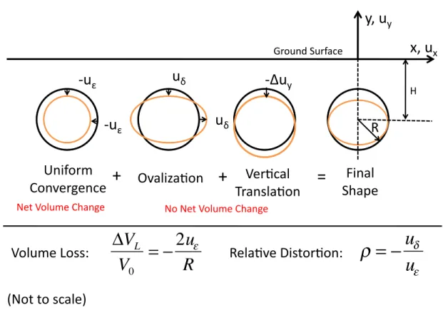
The ‗far-field‘ ground movements caused by shallow tunneling processes (excavation and support) are solved as a linear combination of deformation modes occurring at the tunnel cavity, Figure 3, with input parameters, uε and uδ, corresponding
to uniform convergence and ovalization, respectively. Pinto and Whittle (2011) have shown that closed-form solutions obtained by superposition of singularity solutions (after Sagaseta, 1987) provide a good approximation of the more complete (‗Exact‘) solutions obtained by representing the finite dimensions of a shallow tunnel in a linear elastic soil (after Verruijt and Booker, 1996; Verruijt, 1997).
Pinto et al. (2011) have evaluated the analytical solutions through a series of case studies involving tunnels excavated through different ground conditions using a variety of closed and open-face construction methods. They generally found good agreement with measured data for tunnels constructed in low permeability clays assuming isotropic elastic properties. Although the analytical solutions do not model the actual tunnel construction process, selecting appropriate input parameters can very well capture the net effect of different construction methods. Pinto et al. (2011) noted significant limitations for the case of the Heathrow Express trial tunnel (Deane & Bassett, 1995) and the discrepancies between predicted and measured settlements were attributed to anisotropic stiffness properties of the heavily overconsolidated London Clay.
More recently Gasparre et al. (2007) have presented results from a comprehensive and definitive laboratory investigation of the stiffness properties of natural London Clay using block samples obtained during the excavations for Heathrow Terminal 5. Their test program included measurements of small strain elastic properties (based principally on wave propagation data using triaxial devices equipped with bender elements), limits on the reversible elastic response (referred to as the Y1 yield condition) through drained and 4 5 6 7 8 9 10 11 12 13 14 15 16 17 18 19 20 21 22 23 24 25 26 27 28 29 30 31 32 33 34 35 36 37 38 39 40 41 42 43 44 45 46 47 48 49 50 51 52 53 54 55 56 57 58 59 60
undrained triaxial stress probe tests, and measurements of the degradation of secant stiffness parameters with strain level (using local strain measurements in triaxial and hollow cylinder devices). They conclude that the small strain behavior of the clay is well described by the framework of cross-anisotropic elasticity, and that ‗significant anisotropy was revealed at all scales of deformation‘.
This paper extends the analytical solutions presented by Pinto and Whittle (2011) to account for cross-anisotropic stiffness properties of the clay. The solutions are then evaluated through comparisons with data from the Jubilee Line Extension (JLE) project, involving open-face shield tunnel construction beneath a well-instrumented site in St James Park (Nyren, 1998). This is a very well instrumented and documented case site, with extensive supporting data on cross-anisotropic stiffness parameters for London clay reported by Gasparre et al. (2007). The JLE test section has been extensively analyzed by others using FE analyses and many have reported problems in predicting far-field deformations, and hence, provides an interesting opportunity to assess the capabilities of the proposed analytical solutions. Independent research by Puzrin et al (2012) has attempted to model the same case study using a related analytical approach.
ANALYTICAL SOLUTIONS FOR CROSS-ANISOTROPIC ELASTIC SOIL
The current analyses consider deformations in a vertical plane [x, y] through a cross-anisotropic, linear elastic soil with isotropic properties in a plane with dip angle α to the horizontal as shown in Figure 4. The stiffness parameters of the soil are given for a local [x‘, y‘, z‘] coordinate system (Appendix A shows the transformation to the global frame [x, y, z]). The five independent anisotropic stiffness parameters are defined in the local coordinate system as E1, the Young‘s modulus of the soil at a direction parallel to the isotropic plane, 1 the Poisson‘s ratio of strains in the isotropic plane (x‘-z‘), E2, the Young‘s modulus normal to the isotropic plane, G2, the shear modulus for strain in direction y‘, and ν2, the Poisson‘s ratio for strain in y‘ direction due to strain in the x‘ direction.
Following Milne-Thompson (1960) and Lekhnitski (1977) the stress-strain relations for plane strain geometry conditions can be written as follows:
4 5 6 7 8 9 10 11 12 13 14 15 16 17 18 19 20 21 22 23 24 25 26 27 28 29 30 31 32 33 34 35 36 37 38 39 40 41 42 43 44 45 46 47 48 49 50 51 52 53 54 55 56 57 58 59 60
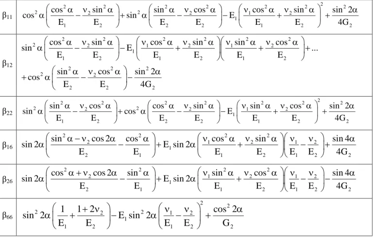
(4a)
where the βij coefficients are related to the 5 independent stiffness parameters and the dip angle α as shown in Table 1. For α = 0° (i.e., isotropic properties in the horizontal plane), Ε1 = Εh, ν1 = νhh, E2 = Ev, ν2 = νvh, G2 = Gvh and the βij coefficients are:
(4b)
where the stiffness ratios n = Eh/Ev and m = Gvh/Ev are used later in the paper.
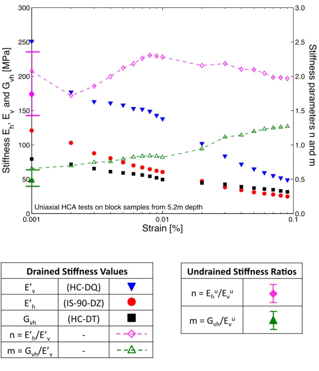
Figure 5 shows non-linear secant stiffness measurements of Ev, Eh and Gvh from drained hollow cylinder (HCA) uniaxial load tests on natural London Clay (unit B2) as functions of strain level (Gasparre et al., 2007). The data show that London Clay is strongly anisotropic at very small strain levels (true elastic range). The stiffness ratio, n = Eh/Ev, varies only slightly, n = 1.72 – 2.30, while m = Gvh/Ev increases from 0.66 to 1.27 with increased strain level. The small strain stiffness ratios calculated from undrained tests are very similar to those from drained parameters as shown in Figure 5.
The elastic parameters are further constrained by thermodynamic considerations (e.g. Pickering 1970) such that:
Gvh, Ev, Eh > 0; 0 < n < 4; -1 < hh < 1; hh + 2 hv vh 1 (4c)
The conditions for incompressibility are given by Gibson (1974) as:
(4d)
In the absence of body forces, the stresses can be solved using the Airy Stress function, F(x, y): (5) x 11 12 16 x y 12 22 26 y 16 26 66 ε ε xy xy
2 2 vh hh 11 12 hh 22 vh 66 16 26 h v v vh 1 1 1 , 1 , 1 n , , 0 E E E G 2 vh hh vh n 0.5, 1 2n 1 2
4 4 4 4 4 22 4 26 3 12 66 2 2 16 3 11 4 F F F F F 2 2 2 0 x x y x y x y y 4 5 6 7 8 9 10 11 12 13 14 15 16 17 18 19 20 21 22 23 24 25 26 27 28 29 30 31 32 33 34 35 36 37 38 39 40 41 42 43 44 45 46 47 48 49 50 51 52 53 54 55 56 57 58 59 60with
Equation (5) is solved by means of the characteristic equation:
(6) The roots of this equation are conjugate complex numbers, say and without loss of generality 1 = a1 + ib1, 2 = a2 + ib2, and b1 > b2 > 0. Any analytic function g(x+y) satisfies eqn. (5) if is a solution to the characteristic equation. Since the resulting stress function must be real, the general solution is given by the following expression:
(7)
where . Introducing the new functions: , the stresses are found using the definition of complex variables z1, z2:
(8a)
(8b)
(8c) and the displacements U(x, y), V(x, y) are found by integrating the strains:
(9a) (9b) where the coefficients pk, qk are expressed as:
(10) 2 2 2 x 2 y 2 xy F F F ; ; y x x y
4 3 2 11 2 16 2 12 66 2 26 22 0 1 2 1, , 2,
1
1 2
2
1
1 1
1 2
2 2
2 F x, y 2 Re F z F z F z F z F z F z 1 1 2 2 z x y, z x y k
zk Fk
zk
2 2
x 2 Re 1 1 z1 2 2 z2
y 2 Re 1 z1 2 z2
xy 2 Re 1 1 z1 2 2 z2
1 1 1 2 2 2
U2 Re p z p z
1 1 1 2 2 2
V2 Re q z q z 2 22 k 11 k 12 16 k k 12 k 26 k p ; q k1, 2 4 5 6 7 8 9 10 11 12 13 14 15 16 17 18 19 20 21 22 23 24 25 26 27 28 29 30 31 32 33 34 35 36 37 38 39 40 41 42 43 44 45 46 47 48 49 50 51 52 53 54 55 56 57 58 59 60Uniform Convergence Mode
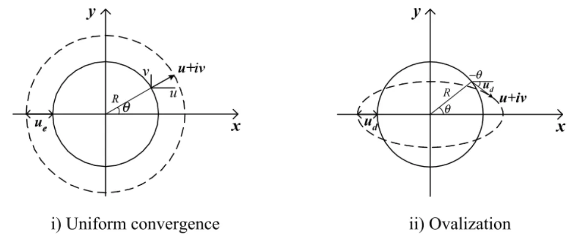
For a cylindrical cavity of radius, R, in an infinite medium undergoing uniform convergence, uε, the displacement components at the tunnel wall can be expressed by (Figure 6a):
(11a)
(11b)
where .
The circular boundary of the tunnel cavity in the [x, y] plane is transformed into an inclined ellipse in the plane of the complex variable (Fig. 6b):
(12a) (12b) The boundary conditions can be solved by a further mapping onto a circle of unit radius as shown in Figure 6b:
(13)
The analytic functions Φk(zk) can be expressed as a Laurent series of the conformed variable k:
(14a)
(14b) At the tunnel wall, | z | = R and 1 = 2 = eiθ = . Hence, from Eqn. 9 the displacement components can be found from:
i i 1 B e e u u cos u u 2 2
i i 1 B e e v u sin u u 2i 2i i e i z x iy Re R
1 1 1 1 1 1 z x y x Re y i Im yx iy
2 2 2 2 2 2 z x y x Re y i Im yx iy
1 2 2 2 2 k k k k k k k k k k k z z R 1 1 i 1 i 1 z R 2 2 R 1 i k 1, 2 1
n 1 1 1 1 1 1 1 n 1 n 0 z z a
n 2 2 2 2 2 2 2 n 2 n 0 z z b
4 5 6 7 8 9 10 11 12 13 14 15 16 17 18 19 20 21 22 23 24 25 26 27 28 29 30 31 32 33 34 35 36 37 38 39 40 41 42 43 44 45 46 47 48 49 50 51 52 53 54 55 56 57 58 59 60(15a)
(15b) Equating the coefficients for powers of ζ:
(16)
The series coefficients are then solved as:
(17)
Ovalization Mode
The ovalization mode involves no ground loss and displacements at the tunnel cavity can be represented as follows:
(18a)
(18b) Applying the same methodology used above (for uniform convergence) the series coefficients an, bn are found:
(19)
The displacements for uniform convergence and ovalization of a circular tunnel in an infinite cross-anisotropic elastic medium are then obtained by combining equations 17 or 19 with equations 14 and 9:
1 n n n n n n 1 n 1 2 n 2 n 0 n 0 n 0 n 0 p a p a p b p b u 2
1 n n n n n n 1 n 1 2 n 2 n 0 n 0 n 0 n 0 q a q a q b q b u 2i
1 1 2 1 1 n 2 n 1 n 2 n 1 1 2 1 u p a p b p a p b 0 2 n 1: ; n 1: q a q b 0 iu q a q b 2 2 2 1 1 1 1 1 2 1 2 1 2 1 2 n n u q ip u q ip n 1: a ; b 2 p q q p 2 p q q p n 1: a b 0
i i 1 B e e u u cos u u 2 2
i i 1 B e e v u sin u u 2i 2i 2 2 1 1 1 1 1 2 1 2 1 2 1 2 n n u q ip u q ip n 1: a ; b 2 p q q p 2 p q q p n 1: a b 0 4 5 6 7 8 9 10 11 12 13 14 15 16 17 18 19 20 21 22 23 24 25 26 27 28 29 30 31 32 33 34 35 36 37 38 39 40 41 42 43 44 45 46 47 48 49 50 51 52 53 54 55 56 57 58 59 60(20a)
(20b)
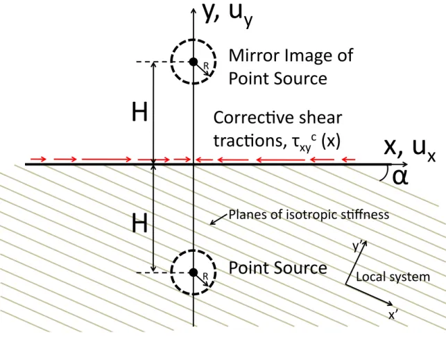
Effect of Traction-Free Ground Surface
Following Sagaseta (1987), the ground movements associated with a shallow tunnel, located at a depth H below the traction-free ground surface can be represented approximately through a singularity superposition technique, Figure 4. The deformation field for the shallow tunnel is represented by superimposing full-space solutions for a point source, [0, -H], and mirror image sink, [0, +H] (i.e., with equal and opposite cavity deformations) relative to the stress-free ground surface (y = 0), respectively:
Contracting tunnel (-uε > 0, uδ > 0):
(21) Mirror image (-uε < 0, uδ < 0):
(22) The resulting normal and shear tractions at the surface y = 0 due to these mirror images are as follows:
(23a) (23b) A set of (equal and opposite) ‗corrective‘ shear tractions Tc
(x) must then be applied at the free surface (Figure 4). The resulting displacements on a half-plane due to these corrective stresses are:
(24) where the analytic functions are obtained through integration (after Lekhnitski, 1977):
1 1
2 1
1 2 1 1 U x, y 2 Re p a p b x, y x, y
1 1
2 1
1 2 1 1 V x, y 2 Re q a q b x, y x, y
x y u x, y U x, y H U x, y H u x, y V x, y H V x, y H
x y u x, y U x, y H U x, y H u x, y V x, y H V x, y H
c y y y y N x x, 0 x, 0 x, H x, H 0
c xy xy xy xy xy T x x, 0 x, 0 x, H x, H 2 x, H
c c c c c c x 1 1 1 2 2 2 y 1 1 1 2 2 2 u 2 Re p z p z ; u 2 Re q z q z c c 1, 2 4 5 6 7 8 9 10 11 12 13 14 15 16 17 18 19 20 21 22 23 24 25 26 27 28 29 30 31 32 33 34 35 36 37 38 39 40 41 42 43 44 45 46 47 48 49 50 51 52 53 54 55 56 57 58 59 60(25a)
(25b) and the integrals of the normal and shear tractions along the boundary are:
(25c)
(25d) Appendix Β summarizes the solution of the infinite integrals in equations 25a, 25b, and 25d from which the following analytical functions are found:
(26a)
(26b)
The final field of ground deformations for a shallow tunnel with uniform convergence at the tunnel cavity is then obtained from equations 21, 22 and 24:
(27a) (27b)
Typical Results
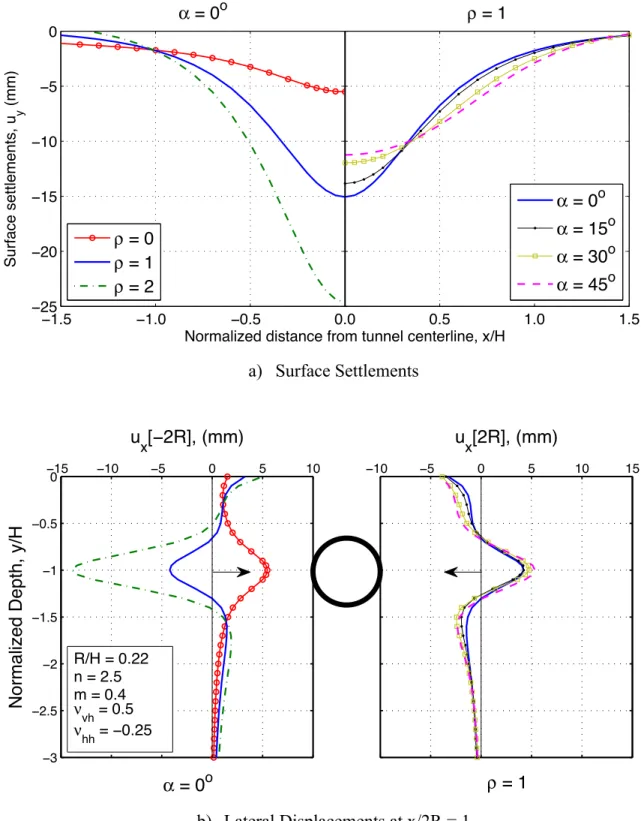
Figures 7 and 8 illustrate the effects of cross-anisotropic stiffness properties on predictions of the shape of the surface settlement trough and lateral deflections for a ‗reference inclinometer‘ offset at a distance x/H = 1 from the tunnel centerline. These results correspond to solutions for undrained deformations (i.e., incompressible conditions with Poisson‘s ratios defined in Eqn. 4d) for a shallow tunnel in clay with R/H = 0.22 (and typical cross-anisotropic stiffness ratios, n and m). Figure 7 shows that for horizontal planes of isotropy (α = 0°), as the ovalization ratio ρ = -uδ/uε increases the predicted settlement troughs become narrower and the surface centreline settlement uy0
2 1
2
c 1 1 1 2 1 f f 1 1 z d 2 i z
1 1
2
c 2 2 1 2 2 f f 1 1 z d 2 i z
s
1 f s N x dx 0
s
s c
2 f s T x dx T x dx
c 1 1 1 1 1 1 2 2 1 2 1 2 2 z z H z H
c 2 2 1 1 2 1 2 2 2 2 1 2 2 z z H z H
c
x x x x u x, y u x, y u x, y u x, y
c
y y y y u x, y u x, y u x, y u x, y 4 5 6 7 8 9 10 11 12 13 14 15 16 17 18 19 20 21 22 23 24 25 26 27 28 29 30 31 32 33 34 35 36 37 38 39 40 41 42 43 44 45 46 47 48 49 50 51 52 53 54 55 56 57 58 59 60increases significantly. For ρ = 0 the analyses predict inward horizontal displacements near the tunnel springline, while increases in ρ result in larger outward movements at this elevation (Fig. 7b). Figure 7 also illustrates results for cases where the plane of isotropy is dipping (α = 0°, 15°, 30°, 45° and ρ = 1), representing (for example) conditions at the edge of a sedimentary basin. As the dip angle increases, the predicted surface centreline settlement uy0 increases, while the effect on the horizontal displacements is less pronounced.
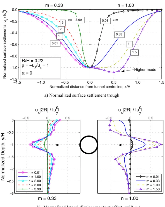
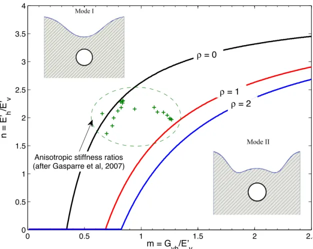
Figure 8 shows the effects of the stiffness ratios, n and m for the case where the soil has isotropic properties in the horizontal plane (α = 0°). The results show a narrowing of the surface settlement trough for normal stiffness ratios, n > 1 (n = Eh/Ev =1 is isotropic case), which is especially pronounced for n > 3. Increases in the shear stiffness ratio, m = Gvh/Ev, have the opposite effect. The settlement trough for m = 1 is much wider than the isotropic case (m = 0.33). There is also a change in the mode shape of the settlement trough shown for m = 1.5, where the maximum settlement does not occur above the centerline, but is instead offset at x/H ≈ 0.5. This result is often observed in 2-D finite element analyses of shallow tunnel excavation for cases with high in-situ K0 stress conditions (e.g., Möller, 2006; Franzius et al., 2005; Addenbrooke et al., 1997), but has not been reported in prior tunneling projects. The transition in mode shape is a function of the anisotropic stiffness ratios (m and n) and the ovalization ratio, ρ, as shown in Figure 9. The subsequent applications of the analyses for the JLE tunnel use a constrained range of ρ to avoid the higher mode solutions.
PRIOR INTERPRETATION OF JLE TUNNEL IN ST JAMES PARK
The Jubilee Line Extension project (JLE, 1994-1999) included 15km of twin, 4.85m diameter, bored tunnels constructed using an open-face shield and excavated by mechanical backhoe. Ground displacements were measured at a well-instrumented greenfield site in St. James‘s Park and were described in detail by Nyren (1998). The Westbound (WB) tunnel passed under the instrumentation site in April 1995 with springline depth, H = 31m and an advance rate of 45.5m/day (i.e., 1.9m/hr). The EB tunnel (not considered in this paper) traversed the section in January 1996 at depth, H = 20.5m (and offset at 21.5m from the WB bore).
4 5 6 7 8 9 10 11 12 13 14 15 16 17 18 19 20 21 22 23 24 25 26 27 28 29 30 31 32 33 34 35 36 37 38 39 40 41 42 43 44 45 46 47 48 49 50 51 52 53 54 55 56 57 58 59 60
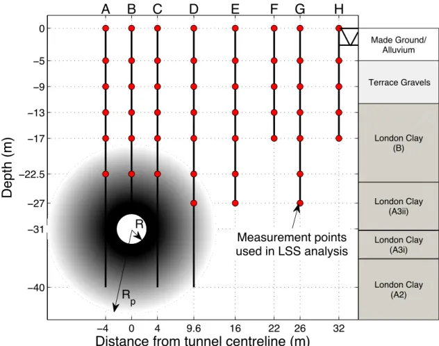
The instrumentation at the test section included an array of 24 Surface Monitoring Points (SMP; surveyed by total stations), while subsurface ground movements were recorded using a set of: 1) 9 electrolevel inclinometers, with tilt angles typically measured at vertical intervals of 2.5m; and 2) 11 rod extensometers, each measuring vertical displacement components at up to 8 elevations. Figure 10 shows eight locations (A-H) where 2D vectors of displacement can be interpreted from the inclinometer and extensometer data.
The soil profile comprises 12m of fill, alluvium and terrace gravels overlying a 40m thick unit of low permeability London Clay (with 4 divisions shown in Figure 10), above the Lambeth Group (lower aquifer system). The groundwater table is located approximately 3m below ground surface but pore pressures are 5 - 7m below hydrostatic at the elevation of the WB tunnel springline. Standing and Burland (2006) have carried out a detailed review of the physical and engineering properties of the four divisions of the London Clay along this section of the JLE alignment. They report the undrained shear strength of London Clay increasing from, su = 215±80kPa (unit A3) to 233±77kPa (A2), and in-situ hydraulic conductivity values, k = 0.15 – 2.0x10⁻¹⁰ m/s.
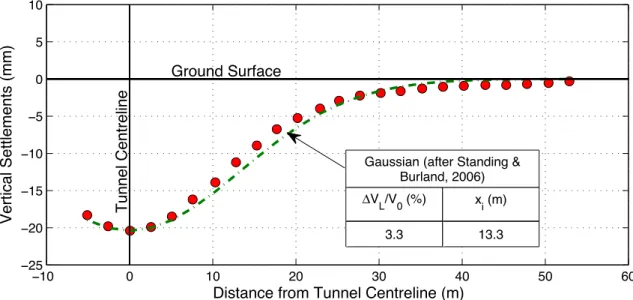
Surface Displacements
Figures 11a and 11b show the vertical and horizontal surface movements measured approximately 1 day after the passage of the WB tunnel face, when it can reasonably be assumed that there is little consolidation within the London clay. Standing and Burland (2006) fitted the transversal surface settlement trough using the empirical Gaussian relation (eqn. 1) with a trough width, xi = 13.3m (i.e., K = xi/H = 0.43) and maximum settlement above the crown, uy0 ≈ 20mm. Hence, the volume loss at the ground surface, ΔVs (=2.5uy0xi) corresponds to an apparent ground loss at the tunnel cavity, ΔVL/V0 = 3.3%, caused by tunnel construction. They attribute this unexpectedly high volume loss to details of the construction method (the WB tunnel was constructed with up to 1.9m of unsupported heading) and to a local ground zone above the WB tunnel crown with a higher concentration of sand and silt partings in the London Clay.
The horizontal surface displacements (Fig. 9b) are also well fitted by conventional empirical assumptions using eqn. 3 with maximum surface horizontal movement ux ≈ 4 5 6 7 8 9 10 11 12 13 14 15 16 17 18 19 20 21 22 23 24 25 26 27 28 29 30 31 32 33 34 35 36 37 38 39 40 41 42 43 44 45 46 47 48 49 50 51 52 53 54 55 56 57 58 59 60
5.7mm at x ≈ 14m east of the centreline. However, it should be noted that the measured profile shows a loss of anti-symmetry (e.g., ux ≠ 0mm at x = 0m) that Nyren (1998) attributes to a deviation in principal stresses acting in the horizontal plane.
Prior Numerical Analyses
Franzius et al (2005) used non-linear finite element analyses to evaluate the measured ground movements reported by Nyren (1998). They compare 2D and 3D analyses, using different coefficients of lateral earth pressure at rest, K0 and various constitutive models for simulating the construction of the JLE WB tunnel. Their base case scenario used a non-linear, isotropic elasto-plastic constitutive model with K0 = 1.5. For an assumed volume loss, ΔVL/V0 = 3.3%, this resulted in a computed maximum surface settlement uy0 = 10mm and a transverse surface settlement trough that was much wider than the measured behavior, Figure 12. Similar results were obtained using 3D analyses with more refined modeling of the tunnel heading.
The Authors modified the constitutive model to include non-linear cross-anisotropic stiffness properties (using a simplified 3 parameter formulation proposed by Graham and Houlsby, 1983). They were only able to achieve good agreement with the measured settlement trough in the 2D analyses using an unrealistically high elastic Young‘s modulus ratio, n = Eh/Ev = 6.5 (i.e., outside the theoretical elastic range of n, eqn. 4b) in combination with a low value of K0 = 0.5. However, when the same model parameters were used in a 3D analysis of the open-face tunnel construction, much larger surface settlements were obtained ( = 85mm with interpreted volume loss, ΔVL/V0 = 18%) as shown in Figure 12.
Wongsaroj (2005) formulated a bespoke constitutive model to describe the non-linear, anisotropic behavior of London clay and used the model in 3D finite element simulations for short and long-term ground movements caused by JLE tunnel construction. Figure 13 compares the measured surface settlements with computed results using four different input parameter sets. Models with both isotropic and anisotropic small strain stiffness (K0 = 1.5; small strain, drained elastic stiffness ratios, n = 0.44, m = 0.13, that are inconsistent with data shown in Fig. 5) resulted in settlement troughs that are wider than the field measurements for the WB JLE tunnel and also
uy0 4 5 6 7 8 9 10 11 12 13 14 15 16 17 18 19 20 21 22 23 24 25 26 27 28 29 30 31 32 33 34 35 36 37 38 39 40 41 42 43 44 45 46 47 48 49 50 51 52 53 54 55 56 57 58 59 60
overestimate significantly the back-figured volume loss (ΔVL/V0 = 5.4% to 6.0%). Good agreement is only achieved by increasing the anisotropic stiffness ratio (Ghh/Gvh = 5 corresponding to m = 0.04) and reducing the assumed value of K0 = 1.2. Figure 13b shows further comparisons with the subsurface horizontal displacements reported by Wongsaroj (2005). The analyses generally predict larger lateral deformations of the soil towards the tunnel centerline than are measured in the field. The Author attributed this discrepancy, in part, to surveying errors in the field measurements. Subsurface horizontal displacements were not reported for the fourth model (Ghh/Gvh = 5) and thus are not shown in Figure 13b.
APPLICATION OF ANALYTICAL SOLUTIONS
The input parameters for the analytical solutions are interpreted from the measured ground deformations of the WB JLE tunnel in St James Park through a least squares fitting approach. The analyses assume linear elastic behavior throughout the soil mass and hence, are likely to underestimate ground deformations close to the tunnel lining where plastic failure occurs in the clay.
This near-field zone of plasticity can be estimated from solutions of a cylindrical cavity contraction in an elastic-perfectly plastic soil (e.g., Yu and Rowe, 1999). The radius of the plastic zone, Rp can be found from:
(28) where N = (p0 – pi)/su is the overload factor, p0 and pi are the pressures in the far field and within the tunnel cavity.
The radius of the plastic zone can then be estimated by 1) equating p0 with the overburden pressure (ζv0 ≈ 600kPa) at the springline, 2) assuming pi = 0; and 3) considering a likely range of undrained shear strength for the London Clay, su = 136 – 293 kPa (A3 unit; Standing & Burland, 2006). Based on these assumptions, Rp ≈ 4 - 13m. The current interpretation excludes measured data within the estimated plastic zone but considers 46 of subsurface deformations (along 8 vertical lines, A-H, Fig. 5) together with 24 locations where surface movements were surveyed. Figure 14 shows the derivation of the least squares solution error (LSS) for the input parameter state space (uε,
p R N 1 exp R 2 4 5 6 7 8 9 10 11 12 13 14 15 16 17 18 19 20 21 22 23 24 25 26 27 28 29 30 31 32 33 34 35 36 37 38 39 40 41 42 43 44 45 46 47 48 49 50 51 52 53 54 55 56 57 58 59 60
uδ), where:
(29) In most practical cases, engineers will expect to fit the measured centerline surface settlement, , and hence, it is preferable to present a modified least squares solution, LSS*, that includes this additional constraint.
Figures 14a and 14b compare results for two sets of soil stiffness properties a) isotropic case (m = 0.33, n = 1, ν = νvh = νhh = 0.5); and b) cross-anisotropic case (with = 0°), based on the small strain behavior reported by Gasparre et al (2007) and assuming incompressibility of the London clay (m = 0.66, n = 2.07, νvh = 0.5, νhh = [1 0.5n] = -0.035). It should be noted that the small strain elastic anisotropic stiffness ratio n = Eh/Ev obtained from undrained tests is very close to that obtained from drained tests as shown in Gasparre et al (2007).
There is little difference in the magnitude of the global least squares error between the two sets of analyses, while the constrained LSS* solution for the isotropic case is slightly closer to the global minimum than the cross-anisotropic case. The derived cavity contraction parameter is smaller for the cross-anisotropic case (-uε = 34mm vs 36mm for the isotropic case), with a lower relative distortion, ρ = -uδ/uε = 1.56 vs 1.32). Both LSS* solutions imply slightly lower volume loss ratios at the tunnel cavity (ΔVL/V0 = 3.0% and 2.8%; Figs. 14a, 14b, respectively) than were estimated by conventional empirical solutions (3.3%; Fig. 11a).
Figure 15 compares analytical solutions of the distributions of vertical and horizontal surface displacement components for the WB JLE tunnel, using isotropic and cross-anisotropic soil properties (with LSS* tunnel mode input parameters). The fields of vertical displacements are very similar for both sets of analyses, while the cross-anisotropic case predicts slightly larger lateral ground movements around the tunnel springline than the isotropic case (Fig. 15b).
Figures 16a and 16b show that both sets of analysis produce very reasonable agreement with the measured vertical and horizontal surface displacements. These results show that reasonable predictions of surface displacements can be achieved using the analytical solutions with isotropic stiffness properties for the London Clay. This is a
2 2
xi xi yi yi i LSSMin
u u u u uy0 4 5 6 7 8 9 10 11 12 13 14 15 16 17 18 19 20 21 22 23 24 25 26 27 28 29 30 31 32 33 34 35 36 37 38 39 40 41 42 43 44 45 46 47 48 49 50 51 52 53 54 55 56 57 58 59 60very surprising result that is due to counteracting effects of the two key stiffness ratios, n and m (cf. Figs. 8a, 8b).
Figures 17a and 17b compare the computed and measured subsurface vertical and horizontal displacement components for the WB JLE tunnel. The computed deformations are generally in very good agreement with both vertical and horizontal components of movements measured in the far field (i.e., outside the expected zone of plastic soil behavior). Very similar patterns of soil displacements are obtained using isotropic and anisotropic elastic stiffness parameters. The analysis tends to overestimate measured centerline vertical settlements below 10m but produce very accurate predictions at the rest of the extensometer positions. The analytical solutions fit well the inclinometer readings at locations from the ground surface up to a transition depth marked by contour line ux = 0mm in Figure 17b, but predict outward movement below this transition depth while the inclinometers show zero ground movements.
CONCLUSIONS
This paper has presented new analytical solutions for estimating 2D ground deformations caused by shallow tunneling in a cross-anisotropic soil. These analyses extend prior solutions derived by Pinto (1999), Whittle and Sagaseta (2003) and Pinto and Whittle (2011) in which the complete distribution of far-field ground movements can be interpreted from two basic tunnel cavity deformation mode parameters (uε and uδ or ρ), the dip angle of the isotopic stiffness plane, , and two key anisotropic stiffness ratios, n = Eh/Ev and m = Gvh/Ev.
The analytical solutions have been applied to re-interpret ground deformations associated with the open-face construction of the WB tunnel for the Jubilee Line at a well-instrumented site in St. James Park (Nyren, 1998). The current analyses benefit from high quality measurements of the cross-anisotropic stiffness properties of intact London Clay measured in an independent study for Heathrow Airport T5 (Gasparre et al., 2007). These data show that London Clay exhibits pronounced stiffness anisotropy at small strain levels.
The cavity deformation mode parameters are evaluated using a least squares fit to surface and subsurface deformations at the instrumented test site. The results show that
4 5 6 7 8 9 10 11 12 13 14 15 16 17 18 19 20 21 22 23 24 25 26 27 28 29 30 31 32 33 34 35 36 37 38 39 40 41 42 43 44 45 46 47 48 49 50 51 52 53 54 55 56 57 58 59 60
both the isotropic and cross-anisotropic analytical solutions produce very good fits to the measured ground displacements. Using the high quality measurements undertaken by Gasparre et al (2007), it can indeed be concluded that cross-anisotropic stiffness parameters have only a small influence on predictions of the far-field ground deformations caused by tunneling in London Clay. The analytical solutions achieve comparable levels of agreement with measurements of the surface settlement trough that are conventionally fitted using an empirical Gaussian distribution function. However, the current analytical solutions correspond to smaller volume losses at the tunnel cavity than those estimated by conventional empirical assumptions (cf., Standing & Burland, 2006) while offering a more consistent framework for interpreting the complete distribution of horizontal and vertical components of ground deformations. Although these results are very encouraging, further case studies are needed to establish how the cavity mode parameters are related to different methods of tunnel construction.
ACKNOWLEDGMENTS
The lead author (DMZ) gratefully acknowledges support provided by the George and Maria Vergottis and Goldberg-Zoino Fellowship programs for her SM research at MIT. This work was initiated through a collaborative project supported by Tren Urbano GMAEC. 4 5 6 7 8 9 10 11 12 13 14 15 16 17 18 19 20 21 22 23 24 25 26 27 28 29 30 31 32 33 34 35 36 37 38 39 40 41 42 43 44 45 46 47 48 49 50 51 52 53 54 55 56 57 58 59 60
REFERENCES
Addenbrooke, T. I., Potts, D. M. & Puzrin, A. M. (1997); ―The influence of pre-failure soil stiffness on the numerical analysis of tunnel construction,‖ Géotechnique, 47(3), 693-712.
Attewell, P.B. (1978); ―Ground movements caused by tunnelling in soil,‖ Proc. Int. Conf.
on Large movements and Structures (ed. J. D. Geddes), Pentech Press, London,
812-948.
Deane, A. P., and Bassett, R. H. (1995); ―The Heathrow Express Trial Tunnel‖. Proc.
Instn. of Civ. Engrs, Geotech. Engng., 113, 144-156.
Franzius, J.N., Potts, D.M. and Burland, J.B. (2005), ―The influence of soil anisotropy and K0 on ground movements resulting from tunnel excavation,‖ Géotechnique, 55(3), 189-199.
Gasparre, A., Nishimura, S., Minh, N.A., Coop, M.R. and Jardine, R.J. (2007); ―The stiffness of natural London Clay,‖ Géotechnique, 57(1), 33-47.
Gibson, R. E. (1974); ―The analytical method in soil mechanics,‖ Géotechnique, 24(2), 115-140.
Graham, J. and Houlsby, G.T. (1983); ―Anisotropic elasticity of a natural clay,‖
Géotechnique, 33(2), 165-180.
Lekhnitskii, S.G. (1963); ―Theory of Elasticity of an anisotropic elastic body,‖ Holden-Day, San Francisco
Mair, R.J., and Taylor, R.N. (1997); ―Bored Tunneling in the Urban Environment,‖
Proceedings of the 14th International Conference on Soil Mechanics and Foundation Engineering, Hamburg, pp. 2353–2385.
Milne-Thompson, L.M. (1960); ―Plane Elastic Systems,‖ Berlin, Springer-Verlag
Möller, S. (2006); ―Tunnel induced settlement and structural forces in linings,‖ Ph.D. Thesis, Institut für Geotechnik, Universität Stuttgart
Nyren, R.J. (1998); ―Field measurements above twin tunnels in London Clay,‖ PhD
thesis, Imperial College, University of London.
O'Reilly, M.P., and New, B.M. (1982); ―Settlements above tunnels in United Kingdom— their magnitude and prediction,‖ Tunnelling 82, London, IMM, 173–181.
4 5 6 7 8 9 10 11 12 13 14 15 16 17 18 19 20 21 22 23 24 25 26 27 28 29 30 31 32 33 34 35 36 37 38 39 40 41 42 43 44 45 46 47 48 49 50 51 52 53 54 55 56 57 58 59 60
Peck, R.B. (1969); ―Deep Excavations and Tunnels in Soft Ground,‖ Proceedings of the
7th International Conference on Soil Mechanics and Foundation Engineering,
Mexico City, State of the Art Volume, pp. 225-290.
Pinto, F. (1999); ―Analytical methods to interpret ground deformations due to soft ground tunneling,‖ SM Thesis, MIT Department of Civil & Environmental Engineering, Cambridge, MA.
Pinto, F. and Whittle, A.J. (2011); ―Ground Movements due to shallow tunnels in soft ground: 1. Analytical solutions,‖ Accepted for publication ASCE Journal of
Geotechnical and Geoenvironmental Engineering.
Pinto, F., Zymnis D.M., and Whittle, A.J. (2011); ―Ground Movements due to shallow tunnels in soft ground: 2. Analytical interpretation and prediction,‖ Accepted for
publication ASCE Journal of Geotechnical and Geoenvironmental Engineering.
Puzrin, A.M., Burland J.B., and Standing, J.R. (2012); ―Simple approach to predicting ground displacements caused by tunnelling in undrained anisotropic elastic soil,‖
Géotechnique, 62(4), 341–352.
Sagaseta, C. (1987); ―Analysis of undrained soil deformation due to ground loss,‖
Géotechnique 37(3), 301-320.
Schmidt, B. (1969); ―Settlements and ground movements associated with tunneling in soils,‖ PhD Thesis, University of Illinois, Urbana.
Standing, J.R. and Burland, J.B. (2006); ―Unexpected tunnelling volume losses in the Westminster area, London,‖ Géotechnique, 56(1), 11-26.
Verruijt, A. (1997); ―A complex variable solution for a deforming tunnel in an elastic half-plane,‖ International Journal for Numerical and Analytical Methods in
Geomechanics, 21, 77-89.
Verruijt, A. & Booker, J. R. (1996); ―Surface settlements due to deformation of a tunnel in an elastic half-plane,‖ Géotechnique, 46(4), 753-756.
Whittle A.J., & Sagaseta, C. (2003); ―Analyzing the effects of gaining and losing ground,‖ Soil Behavior and Soft Ground Construction, ASCE GSP No. 119, 255-291. 4 5 6 7 8 9 10 11 12 13 14 15 16 17 18 19 20 21 22 23 24 25 26 27 28 29 30 31 32 33 34 35 36 37 38 39 40 41 42 43 44 45 46 47 48 49 50 51 52 53 54 55 56 57 58 59 60
Wongsaroj, J. (2005); ―Three-dimensional finite element analysis of short and long-term ground response to open-face tunneling in stiff clay,‖ PhD thesis, University of Cambridge.
Yu, H.S. & Rowe, R.K. (1999); ― Plasticity solutions for soil behavior around contracting cavities and tunnels,‖ International Journal for Numerical and Analytical Methods
in Geomechanics, 23(12), 1245-1279. 4 5 6 7 8 9 10 11 12 13 14 15 16 17 18 19 20 21 22 23 24 25 26 27 28 29 30 31 32 33 34 35 36 37 38 39 40 41 42 43 44 45 46 47 48 49 50 51 52 53 54 55 56 57 58 59 60
APPENDIX A
Rotation of Planes from Local to Global Coordinate System
Considering a cross-anisotropic, linear elastic soil with isotropic properties in a general [x‘, z‘] plane with dip angle α to the horizontal as shown in Figure 4, the strains are related to the stresses in the local [x‘, y‘, z‘] coordinate system through the following relation:
(A1)
The local material compliance matrix Cx‘y‘z‘ is transformed to the global compliance matrix Cxyz as shown below:
(A2) where R is the transformation matrix:
(A3)
2 1 1 2 1 2 2 x 'x ' 2 2 2 x 'x ' y ' y ' 1 2 y ' y ' 1 2 1 z 'z ' z 'z ' x ' y ' x ' y ' 2 x 'z ' x 'z ' y 'z ' 1 y 'z ' 1 2 1 0 0 0 E E E 1 0 0 0 E E E 1 0 0 0 E E E 1 0 0 0 0 0 G 2 1 0 0 0 0 0 E 1 0 0 0 0 0 G x ' y 'z ' x ' y 'z ' C Txyz Cxyz xyz R Cx ' y 'z 'R xyz
2 2
2 2
cos sin 0 0 0 sin 2
sin cos 0 0 0 sin 2
0 0 1 0 0 0
R
0 0 0 cos sin 0
0 0 0 sin cos 0
0.5sin 2 0.5sin 2 0 0 0 cos 2
4 5 6 7 8 9 10 11 12 13 14 15 16 17 18 19 20 21 22 23 24 25 26 27 28 29 30 31 32 33 34 35 36 37 38 39 40 41 42 43 44 45 46 47 48 49 50 51 52 53 54 55 56 57 58 59 60
APPENDIX B
Calculation of corrective stresses integrals
The integral of the tractions along the free surface (eq. 22d) after some manipulation reduces to:
(B1)
The calculation of the stress functions of the corrective stresses , requires the calculation of the infinite integral (eq. 25a):
(B2)
Consider the integrals of the complex functions along the path shown in Figure B1. This path includes branch points for function Fk
(B3)
For small ratios R/H, and usual degrees of anisotropy function the two branch points of the Fk will lie in the upper plane (i.e., outside the chosen integration path) and
therefore the integral of the analytic function Fk according to the Cauchy integral formula
assumes the value:
(B4)
Also: (B5)
The final result is (B6a)
Similarly, (B6b)
2 1 1 1 1 1 1 2 2 2 2 2 2 f s 2 s H s H s H s H , s F1c(z1) F2c(z2)
2 1 2 2 c 1 1 1 2 1 1 2 1 2 k k k k k k k 1 1 2 1 1 f f f 1 1 1 1 z d d 2 i z 2 i z H H 1 1 d d i z z
k w k w , w z w z 2 1,2 k k w HR 1
k k k c c w w dw 2 i z , dw 0 w z w z
R R k k k k R c R I w w dw lim d dw d w z z w z z
c 1 1 1 1 1 1 2 2 1 2 1 2 2 z z H z H
c 2 2 1 1 2 1 2 2 2 2 1 2 2 z z H z H 4 5 6 7 8 9 10 11 12 13 14 15 16 17 18 19 20 21 22 23 24 25 26 27 28 29 30 31 32 33 34 35 36 37 38 39 40 41 42 43 44 45 46 47 48 49 50 51 52 53 54 55 56 57 58 59 60LIST OF SYMBOLS Latin
an Laurent series coefficients
bn Laurent series coefficients
C integration path
E1 Young‘s modulus at the direction parallel to the isotropic plane
E2 Young‘s modulus at the direction normal to the isotropic plane
Eh Young‘s modulus in (any) horizontal direction (plane of isotropy)
Ev Young‘s modulus in the vertical direction
fk(x) integral of traction along boundary
F Airy‘s stress function
G2 Shear modulus for strain in direction normal to the isotropic plane
Ghh shear modulus for strain in the horizontal plane
Gvh shear modulus for strain in (any) vertical plane (planes of anisotropy)
H depth to tunnel springline
i imaginary unit
k hydraulic conductivity
K empirical parameter related to the settlement trough width
K0 coefficient of lateral earth pressure at rest
L radius of integration path
LSS least squares solution
LSS* constrained least squares solution that fits uy0
n, m stiffness ratios
N(x) normal traction on free surface
N overload factor
pk, qk analytic coefficients
p0 pressure outside the tunnel cavity
pi pressure inside the tunnel cavity
R radius of tunnel
Rp radius of plastic zone
s variable 4 5 6 7 8 9 10 11 12 13 14 15 16 17 18 19 20 21 22 23 24 25 26 27 28 29 30 31 32 33 34 35 36 37 38 39 40 41 42 43 44 45 46 47 48 49 50 51 52 53 54 55 56 57 58 59 60
Sk boundary in zk domain
su undrained shear strength
T(x) shear traction on free surface
uδ ovalization parameter
uε uniform convergence parameter ux horizontal ground displacements
horizontal ground displacement measured at point i
uy vertical ground displacements
vertical ground displacement measured at point i
uy0 centerline surface settlement
U, V full space solution (horizontal and vertical displacements)
wk branch points of (w)
x distance from the tunnel centerline
[x, y, z] Global coordinate system
[x’, y’, z’] Local coordinate system
y depth measured from the ground surface
z, zk complex parameters
Greek
α dip angle of plane with isotropic properties
ij coefficients related to stiffness parameters ij shearstrain
ΔVs volume loss at the ground surface
ΔVL/V0 volume loss at the tunnel cavity
i normalstrain
k transformed variable
angle
k roots of the characteristic equation (with positive imaginary part)
Poisson‘s ratio (isotropic case)
1 Poisson‘s ratio for the effect of strains in the isotropic plane (x‘-z‘)
uxi uyi 4 5 6 7 8 9 10 11 12 13 14 15 16 17 18 19 20 21 22 23 24 25 26 27 28 29 30 31 32 33 34 35 36 37 38 39 40 41 42 43 44 45 46 47 48 49 50 51 52 53 54 55 56 57 58 59 60
2 Poisson‘s ratio for the effect of strain in y‘ due to strain in the x‘ direction
hh Poisson‘s ratio for the effect of horizontal on complementary horizontal strain
hv Poisson‘s ratio for the effect of horizontal on vertical strain
vh Poisson‘s ratio for the effect of vertical strain on horizontal strain
integration variable ρ ovalization ratio ζ analytic coefficient i normalstress ζv0 overburden pressure k boundary in k domain ij shearstress k(z) analytic function Superscripts + corresponding to cavity at (0, H) corresponding to cavity at (0, -H) c ―corrective‖ solutions Subscripts B boundary
k integer (assumes values 1, 2)
LIST OF FIGURES
Figure 1: Sources of ground movements associated with tunneling (from Möller, 2006) Figure 2: Empirical estimation of inflexion point (after Mair & Taylor, 1997)
Figure 3: Deformation modes around tunnel cavity (Whittle & Sagaseta, 2003) Figure 4: Superposition method to represent shallow tunnel in cross-anisotropic soil
Figure 5: Anisotropic stiffness ratios from drained HCA uniaxial loading tests on natural London Clay (after Gasparre et al, 2007)
4 5 6 7 8 9 10 11 12 13 14 15 16 17 18 19 20 21 22 23 24 25 26 27 28 29 30 31 32 33 34 35 36 37 38 39 40 41 42 43 44 45 46 47 48 49 50 51 52 53 54 55 56 57 58 59 60
Figure 6a: Prescribed displacement modes at tunnel cavity
Figure 6b: Problem boundaries in zk-plane and in transformed plane
Figure 7: Effect of relative distortion and dip angle on predicted surface settlements and subsurface lateral displacements for cross-anisotropic clay
Figure 8: Effect of anisotropic stiffness ratios (n and m) on predicted surface settlements and subsurface lateral displacements
Figure 9: Effect of anisotropic stiffness ratios and tunnel ovalization ratio on the surface settlement trough mode shapes for shallow tunnels
Figure 10: Cross-section and instrumentation of test section of JLE project in St James's Park – shading indicates plastic zone around tunnel (Rp/R=4-13)
Figure 11: Empirical interpretation of surface displacements for WB JLE tunnel in St. James Park
Figure 12: Surface settlement troughs as predicted by FE analysis undertaken by Franzius et al (2005)
Figure 13: Comparison between field measurements and FE analysis results undertaken by Wongsaroj (2005)
Figure 14: Least squares error analysis undertaken for input parameter selection
Figure 15: Analytical predictions of vertical and horizontal ground deformations for LSS* solutions with isotropic and cross-anisotropic stiffness properties for London Clay
Figure 16: Comparison of computed and measured surface movements for WB JLE tunnel Figure 17: Comparison of computed and measured subsurface ground movements for WB JLE tunnel
Figure B1: Integration path
LIST OF TABLES Table 1: β coefficients used in analytical solution
4 5 6 7 8 9 10 11 12 13 14 15 16 17 18 19 20 21 22 23 24 25 26 27 28 29 30 31 32 33 34 35 36 37 38 39 40 41 42 43 44 45 46 47 48 49 50 51 52 53 54 55 56 57 58 59 60
β11 β12 β22 β16 β26 β66
Table 1: β coefficients used in analytical solution
2 2 2 2 2 2 2 2 2 2 2 2 1 2 1 1 2 2 2 1 2 2
sin cos cos sin
cos sin sin 2
cos sin E E E E E E E 4G 2 2 2 2 2 2 2 2 1 2 1 2 1 1 2 1 2 1 2 2 2 2 2 2 2 2 2
sin cos sin sin cos
cos sin E ... E E E E E E cos sin sin 2 cos E E 4G 2 2 2 2 2 2 2 2 2 2 2 2 1 2 1 1 2 2 2 1 2 2
cos sin sin cos
sin cos sin 2
sin cos E E E E E E E 4G 2 2 2 2 2 1 2 1 2 1 2 1 1 2 1 2 2
sin cos 2 cos cos sin sin 4
sin 2 E sin 2 E E E E E E 4G 2 2 2 2 2 1 2 1 2 1 2 1 1 2 1 2 2
cos cos 2 sin sin cos sin 4
sin 2 E sin 2 E E E E E E 4G 2 2 2 2 2 1 2 1 1 2 1 2 2
1 2
1
cos 2
sin 2
E sin 2
E
E
E
E
G
1. Stress relief at tunnel face 2. Shield over-cut & ploughing 3. Tail Void
4. Deformation of lining 5. Consolidation of soil
A. Deformation at tunnel heading B. Deformation of lining
C. Consolidation of soil
a) Closed-face tunnel b) Sequential excavation Figure 1: Sources of ground movements associated with tunneling
0.0 0.2 0.4 0.6 0.8 1.0 0.0 0.5 1.0 1.5 2.0
Depth Ratio, y/H
Trough Width Parameter, K
R/H Soil Type Site Sym. 0.07 London Clay Green Park 0.06, 0.10 London Clay Regents Park 0.26 London Clay HEX 0.08 London Clay St James Park 0.16 soft clay Willington Qy 0.23, 0.14 kaolin Centrifuge
Mair & Taylor (1997): Clays
Dyer et al. (1996): Sands
Moh et al. (1996): Silty sands
a) Width of surface settlement troughs b) Width of sub-surface settlement troughs Figure 2: Empirical estimation of inflexion point (after Mair & Taylor, 1997)
>u
ε%
>u
ε%
u
δ%
u
δ%
>Δu
y%
+%
Uniform%%
Convergence%
Ovaliza`on%
+%
Transla`on%
Ver`cal%%
=%
Shape%
Final%
R%
H%y,%u
y%
x,%u
x%
Ground%Surface% Net%Volume%Change%ΔV
LV
0= −
2u
εR
No%Net%Volume%Change%Volume%Loss:%
Rela`ve%Distor`on:%
ρ
= −
u
δu
ε(Not%to%scale)%
!"
#$"%
#
"
&$"%
&
"
'())*+,-*"./*0)"
1)0+,(2.$"3
#&+"4#5"
6(721"8(%)+*"
!"
9"
:7))()";<0=*"(>"
6(721"8(%)+*"
? ?#@"
&@"
A(+0B".&.1*<"
6B02*."(>"7.(1)(C7+".,D2*.."
0 50 100 150 200 250 300 Stiffness E h , E v and G vh [MPa] 0.001 0.01 0.10.0 0.5 1.0 1.5 2.0 2.5 3.0 Strain [%]
Stiffness parameters n and m
Uniaxial HCA tests on block samples from 5.2m depth
!"#$%&'()*+%&,,(-#./&,(
!"
#$%&'()*+$
!"
,$%-.(/0()1+$
2
#,$%&'()3+$
4$5$!"
,6!"
#$($
7$5$2
#,6!"
#$($
0%'"#$%&'()*+%&,,(1#*2,(
4$5$!
,86!
#8$
7$5$2
#,6!
#8$
!"#$%&'()*+%&,,(-#./&,(
!"
#$%&'()*+$
!"
,$%-.(/0()1+$
2
#,$%&'()3+$
4$5$!"
,6!"
#$($
7$5$2
#,6!"
#$($
0%'"#$%&'()*+%&,,(1#*2,(
4$5$!
,86!
#8$
7$5$2
#,6!
#8$
Figure 5: Anisotropic stiffness ratios from drained HCA uniaxial loading tests on natural London Clay (after Gasparre et al., 2007)
i) Uniform convergence ii) Ovalization Figure 6a: Prescribed displacement modes at tunnel cavity
−1.5 −1.0 −0.5 0.0 0.5 1.0 1.5 −25 −20 −15 −10 −5 0
Normalized distance from tunnel centerline, x/H
Surface settlements, u y (mm) ! = 0o " = 0 " = 1 " = 2 " = 1 ! = 0o ! = 15o ! = 30o ! = 45o a) Surface Settlements −10 −5 0 5 10 15 u x[2R], (mm) −15 −10 −5 0 5 10 −3 −2.5 −2 −1.5 −1 −0.5 0
Normalized Depth, y/H
u x[−2R], (mm) ! = 0o " = 1 R/H = 0.22 n = 2.5 m = 0.4 #vh = 0.5 # hh = −0.25 b) Lateral Displacements at x/2R = 1
Figure 7: Effect of relative distortion and dip angle on predicted surface settlements and subsurface lateral displacements for cross-anisotropic clay
−1.5 −1.0 −0.5 0.0 0.5 1.0 1.5 −1.2 −1.0 −0.8 −0.6 −0.4 −0.2 0.0
Normalized distance from tunnel centreline, x/H
Normalized surface settlements, u
y / |u y 0 | m = 0.33 n = 1.00 3.99 3 2 0.01 = m n= 0.01 0.33 1 1 1.5 Higher mode R/H = 0.22 ! = −u"/u# = 1 $ = 0
a) Normalized surface settlement trough
−0.5 0 0.5 −3 −2.5 −2 −1.5 −1 −0.5 0
Normalized Depth, y/H
u x[2R] / |uy 0 | m = 0.33 n = 0.01 n = 1.00 n = 2.00 n = 3.00 n = 3.99 −0.5 0 0.5 u x[2R] / |uy 0 | n = 1.00 m = 0.01 m = 0.33 m = 1.00 m = 1.50
b) Normalized lateral displacements at offset, x/2R = 1
Figure 8: Effect of anisotropic stiffness ratios (n and m) on predicted surface settlements and subsurface lateral displacements
0 0.5 1 1.5 2 2.5 0 0.5 1 1.5 2 2.5 3 3.5 4 m = G vh/E’v n = E’ h /E’ v ! = 0 ! = 1 ! = 2
Anisotropic stiffness ratios (after Gasparre et al, 2007)
Figure 9: Effect of anisotropic stiffness ratios and tunnel ovalization ratio on the surface settlement trough mode shapes for shallow tunnels
−4 0 4 9.6 16 22 26 32 −40 −31 −27 −22.5 −17 −13 −9 −5 0
Distance from tunnel centreline (m)
Depth (m) A B C D E F G H R R p Measurement points used in LSS analysis Made Ground/ Alluvium Terrace Gravels London Clay (B) London Clay (A3ii) London Clay (A3i) London Clay (A2)
Figure 10: Cross-section and instrumentation of test section of JLE project in St James's Park – shading indicates plastic zone around tunnel (Rp/R=4-13)
−10 0 10 20 30 40 50 60 −25 −20 −15 −10 −5 0 5 10
Distance from Tunnel Centreline (m)
Vertical Settlements (mm)
Ground Surface
Tunnel Centreline
Gaussian (after Standing & Burland, 2006) !VL/V0 (%) x
i (m)
3.3 13.3
a) Surface settlement trough (after Standing & Burland, 2006)
−10 0 10 20 30 40 50 60 −25 −20 −15 −10 −5 0 5 10
Distance from Tunnel Centreline (m)
Horizontal Displacements (mm)
Ground Surface
Tunnel Centreline
Movements away from tunnel
Movements towards tunnel
Empirically fitted by Eq. 3 u
x = (x/H)uy
b) Surface horizontal displacements
Figure 11: Empirical interpretation of surface displacements for WB JLE tunnel in St. James Park
−10 0 10 20 30 40 50 60 −90 −80 −70 −60 −50 −40 −30 −20 −10 0 10
Distance from Tunnel Centreline (m)
Vertical Settlements (mm) Ground Surface Tunnel Centerline !"#"$%&'(%)%#$&*#*(+,",&-%,.($,/&*0%-&!-*#1".,&%$&*(2&345567& !"#$% &'($)% *"+$#,"'#,% -.% /0!10.%234% #% +% 5,'67'8"9% :*% ;<=% >?<?% ;% .<==% 5,'67'8"9% ?*% ;<=% >:<;% ;% .<==% @#",'67'8"9% :*% .<=% >?<=% A<:=% ;<;B% @#",'67'8"9% ?*% .<=% >;C<;% A<:=% ;<;B% D"$)(%&$E,F7$+$#6,% G
Figure 12: Surface settlement troughs as predicted by FE analysis undertaken by Franzius et al (2005)
−10 0 10 20 30 40 50 60 −25 −20 −15 −10 −5 0 5 10
Distance from Tunnel Centreline (m)
Vertical Settlements (mm)
Ground Surface
Tunnel Centreline
a) Surface settlement trough
!!!!!!!!!!!!!!!!!!!!!!!!!!"#$!!!!!$!!!!!!!!!"#$!!!!!$!!!!!!!!!!!!!"#$!!!!!$!!!!!!!!!!!"#$!!!!!$!!!"#$!!!!!$!!!!!!!!!!!"#$!!!!!$!!!!!!! % &' () !*+ ,! %-.(/01&!234+!5600&7!8&0(3&7-0&!*+,! !!!!!!!!!!!!!!!!!!8!!!!!!!!!!!%!!!!!!!!!!!!!!9!!!!!!!!!!!!:!!!!!!!;!!!!!!!!!!!!<!!!!!!!!
b) Subsurface Lateral Displacements
!"#$%&%'(#)*(+(&'#,&,*-.%.#/(.0*'.1#,2(/#34&5.,/46#7899:;#
!"#$% &'($)% *+% ,--.,/-% 01!.1+%234% #% 5%
67'89':";% <=>% <=+% ?=+% <=+++% +=@A>% B#"7'89':";% <=>% <=>% >=?% +=@AC% +=<A+% B#"7'89':";% <=+% <=>% >=@% +=@AC% +=<A+% B#"7'89':";% <=D% >=+% A=D% +=@AC% +=+AE% F"$)(%&$G7H9$5$#87%
<4%..4&=.#>,?4.@%67'89':";%2IJ/-KIJ--KIJ-/K+=<>4L%B#"7'89':";%&'($)%2IJ/-K+=+MN%IJ--K+=<DN%IJ-/K+=<?4%
n= !vh ' !hv ' " #$ % &' m= n 2 1+ !hh ' ( )"Gvh Ghh # $ % & ' (
Figure 13: Comparison between field measurements and FE analysis results undertaken by Wongsaroj (2005)