Changes in balance coordination and transfer to an unlearned balance task after slackline training: a self-organizing map analysis

Supplemental file 1: SOM training parameters and sensitivity analysis.

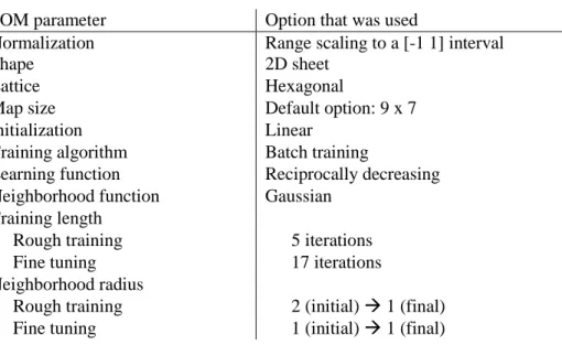
Table S1 shows the SOM parameters that were used in the main manuscript. These correspond to the

default set of options of the SOM Toolbox.

Table S1: Default SOM training parameters.

SOM parameter

Option that was used

Normalization

Range scaling to a [-1 1] interval

Shape

2D sheet

Lattice

Hexagonal

Map size

Default option: 9 x 7

Initialization

Linear

Training algorithm

Batch training

Learning function

Reciprocally decreasing

Neighborhood function

Gaussian

Training length

Rough training

5 iterations

Fine tuning

17 iterations

Neighborhood radius

Rough training

2 (initial)  1 (final)

Fine tuning

1 (initial)  1 (final)

The three measures of SOM quality for this default set of options are given below (definitions from

Kaski and Lagus 1996; Vesanto et al. 2000):

-

Quantization error (QE): average Euclidean distance between normalized input vectors and their

best-matching unit (after the training process): 0.651.

-

Topographical error (TE): percentage of input vectors for which the best-matching unit and

second best-matching units are not neighbours: 0.026 (i.e. 4 trials).

-

Combined error (CE): average Euclidean distance between an input vector and their second

best-matching unit, passing first through the best-matching unit and then through the shortest

path of neighbouring units towards the second best-matching unit: 0.917.

A quality and sensitivity analysis of the SOM methodology was done to assess the robustness of the

analysis performed in the main manuscript. We performed 1728 simulations on the dataset with different

choices for the main training parameters (normalization, shape, lattice, map size, initialization, training

length, training algorithm and neighborhood function). For each simulation, we extracted the SOM

quality measures and the results of the Stuart-Maxwell test of the pre-post contingency table of cluster

membership.

Results showed that the default set of options lay at the 2.34, 1.35

and 9.02

percentiles of QE, TE and

CE respectively. Figures S1-S3 show differences between the options of training parameters in the map

quality. However, the conclusions drawn from the hypothesis tests were not largely affected by the

choice of training parameters. All simulations showed a p < 0.05 for the Stuart-Maxwell test on the

slackline while only 4 simulations (0.23%) showed a p < 0.05 for the flamingo test. These results

demonstrate the strong robustness of the conclusions with respect to the choice of training parameters.

Fig S1: Topological error for all simulations, shown in boxplots per option of each training parameter.

Fig S2: Quantization error for all simulations, shown in boxplots per option of each training parameter.

References

Kaski S, Lagus K (1996) Comparing self-organizing maps. In: von der Malsburg W, von Seelen JC,

Sendhoff B (eds) Proceedings of ICANN96, International Conference in Artificial Neural

Networks, Lecture Notes in Computer Science. Springer, Berlin, pp 809–814

Supplemental file 2: Table showing the mean ± SD of all 45 variables per condition.

Variables Flamingo Slackline

Pre test Post test Pre test Post test

RANGE of MOTION

Ankle pro/supination (°) 17,12 ± 6,54 16,09 ± 4,67 12,77 ± 5,91 16,02 ± 5,75 Ankle plantar/dorsal flexion (°) 5,55 ± 2,17 6,28 ± 2,34 5,52 ± 2,81 6,50 ± 2,42 Knee flexion/extension (°) 11,10 ± 5,39 11,72 ± 5,55 12,46 ± 6,24 13,05 ± 5,48 Hip flexion/extension (°) 17,34 ± 11,43 21,09 ± 12,16 14,96 ± 10,37 20,84 ± 10,75 Hip ab/adduction (°) 24,25 ± 16,52 24,81 ± 12,01 24,43 ± 12,54 30,19 ± 15,15

Pelvis rotation (°) 18,01 ± 10,55 19,05 ± 9,60 16,31 ± 7,00 16,81 ± 7,01

Pelvis lateral tilt (°) 27,46 ± 17,22 28,64 ± 13,72 24,15 ± 10,58 31,57 ± 17,07 Pelvis sagital tilt (°) 9,75 ± 8,33 12,39 ± 7,64 9,74 ± 9,01 12,33 ± 7,43 Trunk rotation (°) 21,59 ± 10,78 25,54 ± 10,01 28,97 ± 12,99 31,69 ± 18,40 Trunk lateral tilt (°) 50,90 ± 25,32 52,93 ± 22,16 55,59 ± 16,54 60,39 ± 23,23 Trunk sagital tilt (°) 16,00 ± 11,70 21,85 ± 19,22 19,00 ± 17,71 23,69 ± 17,07

CoM ant-post (cm) 4,05 ± 1,98 3,78 ± 1,66 3,96 ± 2,12 4,95 ± 1,96

CoM left-right (cm) 4,84 ± 1,72 5,72 ± 2,86 5,96 ± 2,62 5,52 ± 2,42

CoM vertical (cm) 5,58 ± 3,59 7,24 ± 4,46 5,11 ± 3,26 7,25 ± 3,86

VELOCITIES and ACCELERATIONS

Ankle pro/supination (°/s) 11,40 ± 5,58 11,49 ± 4,41 11,06 ± 4,56 10,37 ± 3,93 Ankle plantar/dorsal flexion (°/s) 3,40 ± 1,17 3,78 ± 1,11 4,97 ± 1,66 4,05 ± 1,08 Knee flexion/extension (°/s) 7,98 ± 3,44 7,69 ± 2,80 11,01 ± 4,65 7,79 ± 2,77 Hip flexion/extension (°/s) 8,22 ± 3,33 8,05 ± 3,95 12,80 ± 5,48 7,96 ± 3,57 Hip ab/adduction (°/s) 416,73 ± 598,87 226,21 ± 335,19 463,27 ± 702,69 309,60 ± 45312,

Pelvis rotation (°/s) 8,48 ± 2,85 8,40 ± 3,56 15,78 ± 7,71 10,06 ± 7,26

Pelvis lateral tilt (°/s) 10,56 ± 6,22 10,15 ± 6,40 15,25 ± 5,11 10,49 ± 5,21 Pelvis sagital tilt (°/s) 4,25 ± 1,92 4,46 ± 2,19 6,97 ± 3,68 4,71 ± 2,23

Trunk rotation (°/s) 8,67 ± 4,12 9,93 ± 4,26 18,27 ± 9,13 10,28 ± 5,88

Trunk lateral tilt (°/s) 20,48 ± 9,56 18,18 ± 8,26 29,13 ± 8,06 18,86 ± 6,87 Trunk sagital tilt (°/s) 5,48 ± 3,27 4,83 ± 2,13 8,23 ± 6,33 5,03 ± 2,99

CoM ant-post (m/s) 1,39 ± 0,51 1,39 ± 0,57 2,07 ± 1,04 1,42 ± 0,49 CoM left-right (m/s) 1,65 ± 0,70 1,55 ± 0,57 3,15 ± 1,13 1,77 ± 0,72 CoM vertical (m/s) 2,16 ± 1,02 1,99 ± 0,93 3,52 ± 2,79 2,26 ± 0,89 Head ant-post (m/s²) 18,05 ± 6,80 17,03 ± 5,06 29,59 ± 11,40 18,27 ± 6,38 Head left-right (m/s²) 53,13 ± 23,26 48,87 ± 14,91 90,10 ± 37,09 53,04 ± 27,67 Head vertical (m/s²) 30,11 ± 15,16 28,65 ± 9,66 51,92 ± 22,21 31,85 ± 13,27 FREQUENCIES Ankle pro/supination (Hz) 1,18 ± 0,58 0,96 ± 0,65 1,55 ± 1,08 0,93 ± 0,90 Ankle plantar/dorsal flexion (Hz) 0,95 ± 0,44 0,91 ± 0,56 1,76 ± 1,31 0,99 ± 0,88 Knee flexion/extension (Hz) 1,03 ± 0,48 1,03 ± 0,61 1,91 ± 1,75 0,86 ± 0,69 Hip flexion/extension (Hz) 0,85 ± 0,42 0,69 ± 0,40 2,00 ± 1,88 0,65 ± 0,88

Hip ab/adduction (Hz) 0,63 ± 0,22 0,68 ± 0,50 1,77 ± 1,97 0,60 ± 0,89

Pelvis rotation (Hz) 0,90 ± 0,61 0,79 ± 0,43 1,71 ± 1,43 0,85 ± 0,88

Pelvis lateral tilt (Hz) 0,61 ± 0,21 0,64 ± 0,42 1,31 ± 1,13 0,62 ± 0,89 Pelvis sagital tilt (Hz) 0,78 ± 0,47 0,68 ± 0,42 1,90 ± 1,85 0,84 ± 1,34

Trunk rotation (Hz) 0,81 ± 0,41 0,68 ± 0,38 1,18 ± 0,84 0,64 ± 0,45

Trunk lateral tilt (Hz) 0,56 ± 0,18 0,60 ± 0,43 1,08 ± 0,82 0,46 ± 0,43

Trunk sagital tilt (Hz) 0,60 ± 0,23 0,68 ± 0,55 1,21 ± 0,80 0,67 ± 0,88

CoM ant-post (Hz) 0,62 ± 0,20 0,64 ± 0,45 1,25 ± 1,27 0,59 ± 0,90

CoM left-right (Hz) 0,47 ± 0,21 0,45 ± 0,42 1,11 ± 0,91 0,43 ± 0,91

Supplemental file 3: SOM visualization showing the labels of all trials

Labels: Subject initials – FL/SL – pre/post. Thick black lines show the cluster borders. Numbers

give the cluster number as refered to in the main manuscript.

Example illustrating the count data: subject SA. For the slackline task, she has three trials that

were mapped into cluster 3 at the pre-test, while on the post-test, she has two trials in cluster 4

and one trial in cluster 2. In the slackline contingency table, she thus contributed 3 counts to the

cell c

and 6 counts to the cell c

.

1

2

3