An analysis of sub-band coding techniques for speech communication

AN ANALYSIS OF SUB-BAND CODING TECHNIQUES FOR SPEECH COMMUNICATION

by

ARTHUR JAY BARABELL

SUBMITTED IN PARTIAL FULFILLMENT OF THE REQUIREMENTS FOR THE DEGREES OF

BACHELOR OF SCIENCE and

MASTER OF SCIENCE at the

MASSACHUSETTS INSTITUTE OF TECHNOLOGY October, 1981

) Bell Telephone Laboratories, Inc., 1981

Signature of Author:

Certified by:

Certified by:

..-...-.-. I ,, ....

DeYrtment of Electrical Engineering and Computer Science

"n,'h~ 5 , 1981

· * ' .' . . JA· ·- /6 -. .. . .. . . . .. .. . . . ..

Thesis Supervisor (Academic)

-...

e

I

ooe

*

...

a

*ema

-e

Company Supervisor (VI -A Cooperating Cpmpany)

A

ccepted

by: an..

..

..

er...

tm

en

a...o.

m t.. o-

n.Ga

du.a ude...

Chairman, Departmental-Committee on Graduate Students

An Analysis of Sub-band Coding Techniques for Speech Communication

by

Arthur Jay Barabell

Submitted to the Department of Electrical Engineering and Computer Science on October 5, 1981, in partial fulfillment of the requirements for the degrees of Bachelor of Science and Master of Science.

ABSTRACT

Sub-band coding has been proposed as an efficient means of

encoding signals for digital transmission. In this thesis, an analysis is presented of the various techniques used in the implementation of sub-band coders. An efficient scheme, due to Crochiere, for implementing pitch prediction in sub-band coders is presented, as well as a discussion on the design and analysis of such pitch prediction systems.

New designs for 9. 6 kb/s and 16 kb/s sub-band coders are presen-ted. These coders were simulated on a general purpose digital

computer. The objective and subjective performance of the simulated coders is discussed, and comparisons are made with the performance of previous designs. Since these new sub-band coders are the first to incorporate pitch prediction, particular attention is paid to the improve-ment in performance due to the use of pitch prediction. Suggestions are made for obtaining further improvements in sub-band coder performance.

Thesis Supervisor: James H. McClellan

Title: Associate Professor of Electrical Engineering Thesis Supervisor: Ronald E. Crochiere

Title: Member of Technical Staff, Bell Telephone Laboratories

-2-ACKNOWLEDGEMENT

Many people have helped to make this thesis a worthwhile experience, and I would like to acknowledge their contribution.

The bulk of the thesis research was done at the Acoustics Research Department of Bell Laboratories, under the auspices of the MIT cooperative program in Electrical Engineering and Computer Science.

I would like to express my deepest appreciation to Dr. Ronald E. Crochiere, my thesis supervisor at Bell Labs, for all the advice and encouragement that he provided throughout the course of this project. I would also like to thank Dr. James L. Flanagan for not only making the facilities of his department available to me, but also for-several suggestions which enhanced my understanding of speech processing. I would also like to acknowledge the contributions of James D. Johnston, who made numerous suggestions on the design of the systems simulated, and Carol A. McGonegal, who helped me cope with the computer system.

Several people at MIT also made valuable contributions to this thesis. Dr. Michael R. Portnoff read and commented on the thesis proposal, and his help was much appreciated. Professor James H. McClellan was kind enough to read the various drafts of this thesis

document. His comments and suggestions have greatly enhanced the clarity of the presentation.

Finally, I would like to thank Mrs. Delphine Radcliffe for the super job she did in typing the manuscript.

TABLE OF CONTENTS Page ABSTRACT .. . . . . . A CKNOWLEDGEME NTS TABLE OF CONTENTS LIST OF FIGURES . . . . .. CHAPTER 1 INTRODUCTION . 1. 1 Introduction

1.2 The Scope of This Thesis

. . 11

.... 11

. . . . 15

CHAPTER 2 BAND-SPLITTING AND FREQUENCY

TRANSLATION METHODS .

...

2. 1 Introduction

2. 2 Selection of Sub-band Widths

and Locations .

..

2.3 Integer Band Sampling . .1. . . 18

2.4 Integer Band Sampling Incorporating

Quadrature

Mirror Filters .

.

2.5 The Use of QMF's to Obtain Octavely

Spaced Sub-bands .

....

2.6 Efficient Implementation of QMF-Based Splitting-Decimation and Interpolation-Merging Networks 2.7 Relative Computational Costs of

Implementing Conventional vs QMF-Based Bandsplitting-Decimation and Interpolation-B andmerging Networks

CHAPTER 3 THE USE OF PITCH PREDICTION IN SUB-BAND CODING ...

3. 1 Introduction · · I I G · 0 0

3.2 Predictive Encoding .

.

.

3. 3 Pitch Prediction .

. .

.

3.4 The Use of Pitch Prediction in

Sub-band Coders . .. ..

3.5 Pitch Prediction of Band-pass Decimated

Speech . . . . .

-4-2 3 4 6 17 * . 17 17 23 43 48 51 56 56 56 64 67 70 r·r· c·c· * · · · r · * -. * * * *

TABLE OF CONTENTS (continued)

Page 3. 6 The Practical Use of Pitch Prediction

in Sub-band Coders .

.

.

3. 7 Considerations in the Design of Band-pass Filters for Use in Digital

Phase Shifters .

..

.

3. 8 Efficient Implementation of the Phase

Shifter . . . .

3. 9 Computational Costs of Implementing

Pitch Prediction .

.

76

83 106 109

CHAPTER 4 QUANTIZATION OF SUB-BAND SIGNALS .

4. 1 Introduction .

....

.

4.2 Adaptive Quantization

4.3 Modifications to the APCM Algorithm 4.4 Bit Allocation

CHAPTER 5 SIMULATION OF 9.6 kb/s AND 16 kb/s SUB-BAND CODERS INCORPORATING

PITCH PREDICTION .

..

· 122

127

5. 1 Introduction .

...

5.2 The Basic System

5. 3 Performance of the Sub-band Coder

Systems: Preliminary Results

-Objective Measurements

5.4 Performance of the Sub-band Coder Systems: Preliminary Results -Listening Comparisons

CHAPTER 6 SUMMARY AND SUGGESTIONS FOR IMPROVING SUB-BAND CODER

PERFORMANCE . . . .

6.1 Summary . . . . 6

6.2 Suggestions for Improving Sub-band

Coder Performance ..

.

REFERENCES 112 112 112 118 127 127 137 ·· . 141 143 143 143 147 * . * * * * * * · * * * · · n···

LIST OF FIGURES

CHAPTER 1

Fig. 1. 1(a) Fig. 1. 1 (b)

Transmitter section of a generic sub-band coder. Receiver section of a generic sub-band coder.

CHAPTER 2 Fig. 2. 1(a)

Fig.

Fig. Fig. Fig.

Fig.

Fig.

2. 1(b) 2. 1 (c) 2.2 2. 3 2.4(a) 2. 4(b) Fig. 2.5(a) Fig. 2.5(b) Fig. Fig. 2. 6 2. 7(a) Fig. 2. 7(b) Fig. 2. 8(a) Fig. 2.8(b)

Implementation of sub-band coder based on integer band sampling.

Decrease in sampling rate by a factor D..

1

Increase in sampling rate by a factor Di. A frequency domain interpretation of integer band sampling.

Parameters of the bandpass filters. A two-band sub-band coder.

Frequency response of typical quadrature

mirror filters.

Frequency response of a 16-tap low-pass Hanning filter designed for use in a two-band QMF-based sub-band coder.

Overall frequency response of the two-band QMF-based sub-band coder of Fig. 2.4(a) implemented with the filter of Fig. 2. 5(a).

(Note the difference in amplitude scale between Figs. 2.5(a) and 2. 5(b).)

Four-band sub-band coder incorporating QMF's. Transmitter section of five-band sub-band

coder incorporating QMF s.

Receiver section of five-band sub-band coder incorporating QMF's. Decimator-bandpass bandpass-decimator equivalence. Bandpass-interpolator - interpolator-bandpass equivalence. Page 14 14 19 19 19 20 22 25 25 32 32 36 37 38 40 40

LIST OF FIGURES (continued) Page Fig. 2.9 Fig. 2.10 Fig. 2.11(a) Fig. 2. 11(b) Fig. 2.12(a) Fig. 2. 12(b) Fig. 2.13(a) Fig. 2.13(b) Fig. 2. 13(c) Fig. 2. 14(a) Fig. 2.14(b) Fig. 2.14(c)

Equivalent parallel structure for coder

of Fig. 2.6.

Equivalent parallel structure for coder

of Fig. 2. 7.

Sub-band widths and locations for two 16 kb/s sub-band coders (i) old coder of Reference [3] (ii) new coder proposed in this thesis.

Sub-band widths and locations for two 9.6 kb/s sub-band coders (i) old coder of Reference [3] (ii) new coder proposed in this thesis.

Bandsplitting-decimation structure for genera-ting four octavely-spaced sub-bands.

Interpolation-merging structure for recon-structing the full band from four octavely-spaced sub-bands.

Two band bandsplitting-decimation network incorporating QMF' s.

Equivalent structure for Fig. 2. 13(a). Efficient implementation for Fig. 2, 13(c) (after Croisier et al. [12]).

Two-band interpolation-bandmerging net-work incorporating QMF's.

Equivalent structure for Fig. 2.14(a). Efficient implementation for Fig. 2.14(c)

(after Croisier et al. [123).

CHAPTER 3

Fig. 3.1 (a)

Fig. 3. 1(b)

Fig. 3.1(c) Fig. 3.2(a)

Predictive encoding system.

Predictive encoding system of Fig. 3. 1(a) incorporating quantization noise source model.

Equivalent for the system of Fig. 3. l(b). Predictive encoding system incorporating feedback around the quantizer.

41 42 44 45 46 47 49 49 49 50 50 50 57 59 59 61

LIST OF FIGURES (continued) Page Fig. 3.2(b) Fig. 3.2(c) Fig. 3.3(a) Fig. 3. 3(b) Fig. 3.4 Fig. 3.5

Fig.

Fig.

3. 6 3. 7 Fig. 3.8

Equivalent for system of Fig. 3.2(a), incorpor-ating quantization.noise source model.

Equivalent for system of Fig. 3.2(b).

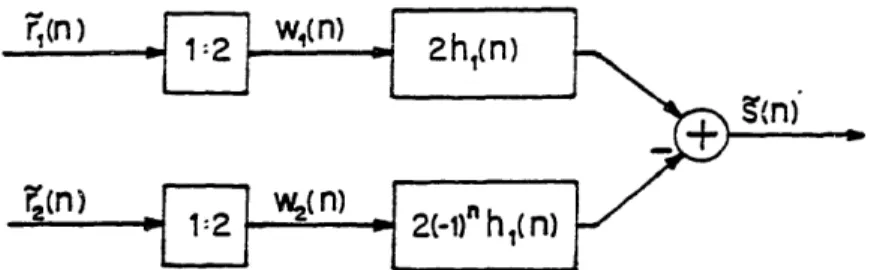
Pitch predictive coding system (after

Crochiere [71).

Pitch predictive coding system incorporating feedback around the quantizer (after

Crochiere [7]).

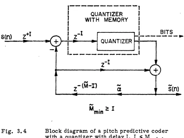
Block diagram of a pitch predictive coder with a quantizer with delay I, I Mmin*

(after Crochiere [7])

Sub-band coder with separate pitch prediction loop around each sub-band (after Crochiere

[7]).

Band i of the pitch predicting sub-band coder of Fig. 3. 5 (after Crochiere [7]).

Predictive encoding of downsampled sub-band signals.

One band of sub-band coder incorporating pitch prediction of downsampled sub-band signals (after Crochiere [7]).

Fig. 3. 9

Fig. 3.10

Fig. 3.11

Fig. 3. 12

Fig. 3.13(a)

Detailed view of digital phase shifter (after Crochiere [7]).

Equivalent for system of Fig. 3. 8 (after Crochiere [7]).

Terminal-analogue model of the vocal system (after Schafer and Rabiner [26]).

A series of amplitude spectra representing a vowel segment [ae]. Time runs from top to bottom (after Fujimura [27]).

Relationship of the linear phase shift at the high sampling rate to the phase shift at the sub-band sampling rate for the r = 1 sub-band. Fig. 3.13(b) Relationship of the linear phase shift at the

high sampling rate to the phase shift at the sub-band sampling rate for the r = 2 sub-band.

-8-62 62 65 65 68 69 71 73 74 75 77 78 80 87 88

LIST OF FIGURES (continued) Page Fig. 3. 14(a) Fig. 3.14(b) Fig. 3. 15 Fig. 3.16 Fig. 3.17 Fig. 3.18(a) Fig. 3.18(b) Fig. 3.18(c) Fig. 3.19

Bandpass filter response for r = 2, D = 4 sub-band system.

Resulting terms of sum in Equation (3.13) using filter of Fig. 3. 14(a) (see text). Model for determining the effect of filter passband ripple on the pitch prediction

system performance.

Effect of passband ripple on pitch prediction performance when ripple structure is

aligned with pitch harmonic structure. Magnitude response of a bandpass filter designed to isolate the r = 1 sub-band in a

D = 8 bandpass interpolator.

Phase shifter response for D = 8, r = 1, M = 40, using the bandpass filter of Fig. 3.17.

Phase shifter response for D = 8, r = 1, M = 43, using the bandpass filter of Fig. 3.17.

Phase shifter response for D = 8, r = 1, M = 46, using the bandpass filter of

Fig. 3.17. I00

Magnitude response of the bandpass filters used to implement the pitch predicting

phase shifters in the proposed 9.6 kb/s and

16 kb/s sub-band coders. 105

107 Fig. 3.20(a) Detailed view of digital phase shifter

(after Crochiere [7]). Fig. 3.20(b)

Fig. 3.20(c)

Equivalent for system of Fig. 3.20(a). Equivalent for system of Fig. 3. 20(b).

CHAPTER 4 Fig. 4. 1 Fig. 4. 2

Block companded PCM (BCPCM) principle (after Esteban and Galand [4]).

Step-size adaptation algorithm and quantizer characteristics of the APCM coders (after Crochiere [3]).

90 91 93 94 97 98 99 107 107 114 115

LIST OF FIGURES (continued)

Page General shape of optimal multiplier function

for APCM coders in speech quantization;

B > 2 (after Jayant [9]).

Two common uniform quantizer

character-istics; (a) mid-tread (b) mid-rise (after

Rabiner and Schafer [18]).

The modified mid-tread quantizer character-istic obtained when the lowest magnitude output levels of the characteristic of Fig. 4.4(b) are switched to zero.

Comparison of bit allocations and resulting sub-band SNR's for new sub-band coders and old sub-band coders of Reference [3].

123 125 CHAPTER 5 Fig. 5. 1(a) Fig. 5.1 (b) Fig. 5.2(a) Fig. 5.2(b)

Transmitter section of the new sub-band coders which were simulated.

Receiver section of the new sub-band coders which were simulated.

Comparison of frequency response for new 16 kb/s sub-band coder and old 16 kb/s coder of Reference [3].

Comparison of frequency response for new

9. 6 kb/s sub-band coder and old 9. 6 kb/s

sub-band coder of Reference [3].

-10-Fig. 4.3

Fig. 4.4

Fig. 4.5 Fig. 4.6 117 121 128 129 135 135

CHAPTER 1

INTRODUCTION 1. 1 Introduction

The advantages of digital coding of signals are well known and widely discussed in the literature. Some of these advantages include robustness, efficient signal regeneration, the possibility of combining transmission and switching functions, and easy encryption. However, in achieving these benefits, one must pay a price - digital signals, such

as PCM signals, have greater transmission bandwidth and storage requirements than their analog counterparts. Thus, there has been a great amount of research interest in the efficient coding of digital

signals. A substantial portion of this continuing effort is devoted to the coding of digital speech signals [1].

The speech coding systems which have been devised fall into several categories. At one end of the spectrum [sic] are waveform coders. Waveform coders attempt to reproduce the signal waveform, traditionally taking advantage of only a few properties of the signal being encoded (i. e. finite bandwidth, finite dynamic range, some correlation between successive samples, etc.). Thus, these schemes may be used for a large variety of signals - speech, music, and video - to cite a few examples. These algorithms are capable of yielding coded signals which are robust with respect to transmission and storage errors.

Furthermore, the original signal may be reproduced with virtually any fidelity required by increasing the number of bits used to encode each

sample. However, these algorithms are not very efficient - they require rather high bit rates (e. g. 56 kb/s for log PCM) to reproduce toll quality speech [1].

At the opposite end of the speech coder spectrum [sic] are vocoders, which attempt to analyze the original speech signal, and transmit the parameters of a speech production model for future regeneration. The fidelity of the reproduced signal to the original is very much dependent upon the accuracy of the model. In addition, vocoded speech signals are very error sensitive, due to their low

redundancy. Even under error-free conditions, vocoded speech sounds rather unnatural, due to the failure of even current state-of-the-art

models to fully characterize the human speech mechanism. However, vocoders are capable of yielding intelligible speech at bit rates as low as

500 b/s (for formant vocoders).

From the brief discussion above, one can see that neither wave-form coders nor vocoders would entirely satisfy the requirements of a digital speech transmission sstem for use over stadard telephone lines; fairly high quality speech at 4. 8 kb/s to 16 kb/s in a transmission environment which is not error-free. Thus, much recent research has been focussed on coding schemes which exploit speech and hearing

models, without making the algorithm totally dependent on these models. The redundancy in speech due to the vocal tract filtering action can be removed in the time domain by exploiting the resulting correlations between successive speech samples. Alternatively, this redundancy can be removed in the frequency domain by exploiting the quasi-stationary, nonuniform nature of the short-time spectral envelope of speech signals.

The redundancy in speech due to the quasi-periodic nature of voiced speech can be removed in the time domain by exploiting the

correlation between speech segments one or more pitch periods apart. Alternatively, this redundancy can be removed in the frequency domain

-12-by exploiting the spectral fine structure associated with the harmonics of the pitch frequency.

Sub-band coding [2-5] efficiently exploits the redundancies in speech due to the vocal tract filtering process. In addition, sub-band coding exploits models for auditory perception.

A generic sub-band coder is shown in Fig. 1. 1. In this figure, s(n) is the discrete time representation of a bandlimited signal which has been sampled at the Nyquist rate. This discrete time signal is split into a number of sub-band signals, typically four to eight, by the bank of band-pass filters. Each sub-band signal is translated down to dc and then re-sampled at the Nyquist rate for that sub-band. It is these base-band signals which are separately encoded, multiplexed, and then trans-mitted. At the receiver, the bit stream is demultiplexed and decoded. The sub-band signals are reconstructed at the original, higher sampling rate, band-pass translated to the proper frequency, and then added, to produce a facsimile of the original speech signal.

By allowing the quantizers' step-sizes to adapt independently according to the signal level in each sub-band, the coder takes advantage of the quasi-stationarity and nonuniformity of the short-time spectral envelope of speech. Since quantizing noise produced in each sub-band is localized to that sub-band, signals in one sub-band will not be masked by the quantizing noise produced by another sub-band. The total number of bits available may be allocated to each band according to perceptual

criteria. Dynamic bit allocation schemes have been proposed [5] which

Although it is useful to think of these seps as being physically separate, in practice one combines their implementation to achieve the same results with fewer operations.

Fig. 1. l(a) Transmitter section of a generic sub-band coder.

periodically update the bit allocation according to the spectral content of the signal being coded.

1. 2 The Scope of this Thesis

The sub-band coders proposed by Crochiere et al. [2, 3] and Esteban and Galand [4, 51 have demonstrated the ability to produce toll quality speech using 24 kb/s systems and communications quality speech using 9.6 kb/s systems [1,6]. The new 9.6 kb/s and 16 kb/s sub-band coders designed and simulated on a general purpose digital computer as part of this thesis project make use of a combination of techniques

previously demonstrated by the researchers cited above. In addition, the proposed coders exploit the quasi-periodic nature of voiced speech using an efficient pitch prediction technique proposed by Crochiere [7]. An important goal of this thesis is to evaluate the improvement in

performance due to the use of pitch prediction, since these are the first sub-band coders to make use of such systems. The thesis is organized as follows:

Chapter 2 is concerned with methods for the division of the

original, full band speech signal into several baseband sub-band signals. The discussion includes considerations on the choice of sub-band loca-tions and widths, a presentation of efficient systems for the conversion of the full band signal into several sub-bands, a treatment of the design of filters for use by these systems, and a comparison of the computa-tional costs of implementing these techniques.

Chapter 3 is concerned with the use of pitch prediction in sub-band coding. The chapter begins with a brief discussion of time domain methods for predictive coding, and then focusses on the specific example of pitch predictive coding. This discussion is followed by a presentation

of an efficient technique (due to Crochiere [7]) for the implementation of pitch prediction in sub-band coders. The description of this technique

is followed by a discussion on the practical design of such systems, and some constraints on their performance. Some of these constraints are due to the particular prediction and sub-band coding systems imple-mented, while other constraints are due to the properties of voiced

speech signals. The chapter concludes with a consideration of the com-putational costs of adding pitch prediction to a given sub-band coding system.

Chapter 4 presents a discussion on quantization techniques and bit allocation issues in sub-band coders. Since the quantization techniques are widely discussed in the literature [1, 8-11], this discussion is

relatively brief.

The first part of Chapter 5 is devoted to a presentation of the final design configurations for the 9. 6 kb/s and 16 kb/s sub-band coders which were simulated. The second part is devoted to the consideration

of the simulation results. This consideration focusses on two topics: the improvement in coder performance due to the utilization of pitch predictive encoding, and comparisons on the subjective performance of the proposed coders and the earlier coders of Crochiere [3].

Chapter 6 concludes the thesis with a summary of the major results and some suggestions for the improvement of the proposed sub-band coders.

-16-CHAPTER 2

BAND-SPLITTING AND FREQUENCY TRANSLATION METHODS 2. 1 Introduction

This chapter begins with a brief discussion on the selection of sub-band widths and locations. Following this discussion is a presenta-tion of a general method of bandsplitting and frequency translapresenta-tion,

commonly referred to as integer-band sampling [2, 3]. Also presented in this chapter is an important sub-class of this method, which incorpor-ates the so-called "Quadrature Mirror Filters" (QMF's) [4, 5, 12].

Filter design considerations for these methods are presented. The chapter concludes with a comparison of the computational costs of implementing integer-band sampling with either conventional filters or QMF's.

2. . Selection of Sub-band Widths and Locations

In choosing the locations and widths of the sub-bands, one may be guided by the concept of an articulation index (AI) [13, 14]. The Al

specifies the division of the frequency scale into twenty nonuniform con-tiguous bands, where each "articulation band" contributes equally to the average total intelligibility of speech. Thus, the sub-bands of the system are allocated so that each sub-band contains an equal number of "articulation bands", then each sub-band will make an equal contribution to the intelligibility of the system. As will soon be demonstrated, the method chosen for band -splitting may restrict the ability of the designer to meet this requirement. Fortunately, however, little loss in perform-ance is perceived if this equal contribution to intelligibility constraint is

2. 3 Integer Band Sampling

There are various techniques available for the translation and re-sampling of the sub-band signals. Several of these schemes are discussed in Reference [2]. Figures 2. 1 and 2. 2 illustrate the imple-mentation of a sub-band coder based on integer band sampling. The speech band is partitioned into N sub-bands by band-pass filters BP1 to

BPN . The speech signal s(n) is assumed to be a discrete-time signal

m. (m.+ 1) The pass-band of BP. has lower and upper limits of j7r and

i i

respectively, where mi and D. are integers, and m. + 1 D.. Thus,

when filter output si(n) is down-sampled by the factor Di, practically no

information is lost due to aliasing (assuming, of course, that the band-pass filter is good enough, as will be discussed later in this section). This process of band-pass filtering followed by a sampling rate reduction

is commonly referred to in the literature as band-pass decimation [15]. The sub-band signals r (n) through rN(n) are encoded and then multiplexed for transmission over a single channel. At the receiver, the channel signal is demultiplexed and decoded. The sampling rate of each sub-band signal riW(n) is increased back to the original rate by inserting zeros and the resulting signal wi(n) is interpolated by filtering with another band-pass filter, identical to BP.. This filter needs to have a gain of Di to compensate for the signal energy which was lost in

the decimation process. The process of increasing a signal's sampling rate, followed by band-pass filtering is known as band-pass interpolation [15]. The filter outputs sl(n) to sN(n) are then summed together to form a facsimile of the original speech signal.

Integer band sampling is preferable over other techniques for frequency translation and resampling because it eliminates the need for modulators. This technique can be made to be even more efficient if the

-18--4 CJ 0 +1 +1 C) Ii I

E

'f "' Om C 02 C C a * el _C1C Q.0 . I C* a ._, oC e _s~~~~~r.~~~ ~._

XY

a

*_5-ut I 11 -1

Ll WI-JIO Z cJ z (D n J

z

CD Z) C H I-:) 2

0

C.) 13: .4 C 0 o C_C r= a) S-4 c:CV ._I '0

3

_{_21}

3

_a .4 .-+

0

4-<I) cn 0

z

m Af w

it

:

3

-j

CD V5

4

_z

(D C) CO C,I

0

2

co a. ci) C z -m C -C

?g

r- u

0

w Z

0

z

-C

-a

,03 _ a -cn rN I w

a

2

0

2

C 4: +

EI

L

O

i

F1f

-I 3 Cn

-20-t

It 'V I

band-pass filters are implemented using nonrecursive (i. e. Finite Impulse Response (FIR)) designs. When using a nonrecursive filter in the band-pass decimator, only one out of every Di filter output samples

need be computed; these are the only samples that will remain after the

decrease in sampling rate. In contrast, when recursive filters are

employed in band-pass decimators, every filter output point must be computed, since the desired filter output points depend on all the past filter outputs. At the band-pass interpolator, D. - 1 out of every Di₁

!

input samples to the filter is zero; hence these samples do not affect the computation [15] when nonrecursive filters are used.

When using integer-band sampling, it will not be possible to select the sub-band widths and locations to exactly satisfy the equal AI contribu-tion criterion. This restriction is due to the requirement that sub-bands

m. f m.+ lf

lie between

4

T and

-2

,

where f is the original full-band

1 1

sampling rate, mi and D. are integers, and m. < D.. In practice, the slight relaxation of the equal AI contribution criterion has only a slight degrading effect on the sub-band coder performance [3].

In designing the band-pass filters BP1 through BPN, one must

take into account several considerations. As shown in Fig. 2. 3, during the decimation process in the transmitter, signal frequencies outside the sub-band are aliased into the sub-band. For this aliasing effect to go unperceived, the stop band attenuation of the band-pass filters must be considerable; in practice, on the order of 45 dB [3]. Due to the filter's finite transition region, the filter pass-band must have a slightly

narrower frequency range than the sub-band width, in order to minimize aliasing effects at the edges of the sub-band. Filter attenuations of 12 dB at the sub-band edges will leave the aliasing effects unperceived,

0

0

0

c's o O I o o LO u 0 (D o i I I i (SP) 3anGlIdV

-22-U; *-4 cn a "O e a,

,:

U CU Cl)

z

5

_x

0

z

Lzjb CY ui mt Lr, mu

as they are being confined to a very narrow frequency region [3]. When 175 - 200 tap FIR filters are used, it is possible to obtain the above

requirements with a pass-band ripple of t 0. 5 dB and a Aw of 0. 01 r radians, which corresponds to 50 - 60 Hz when sampling rates of 9. 6 to 10. 67 kHz are used, as in Reference [3]. If the different sub-bands are contiguous, the resultant gaps in the overall system frequency response will cause the coder to have a reverberant quality. To minimize this reverberance, it is possible to overlap the sub-bands slightly, and

obtain a smoother frequency response. However, this will increase the channel bandwidth requirement, which for a fixed bit-rate means reduc-ing the number of bits available for quantization, resultreduc-ing in an increase in quantization noise. For the five-band, 16 kb/s coder of Reference [3], the lower bands are overlapped slightly, while the upper sub-bands are contiguous. For the four-band, 9. 6 kb/s coders of Reference [3], the lower sub-bands are contiguous, while the upper sub-bands have gaps between them in order to conserve transmission bandwidth. The subjective quality of these systems will be discussed in Chapter 5. 2.4 Integer Band Sampling Incorporating

Quadrature Mirror Filters

As discussed in the previous section, the necessity of minimizing aliasing effects forces the designer to compromise between computation load (which depends on the band-pass filter order), reverberance, and noise level. In some cases, however, it is possible to utilize

"Quadrature Mirror Filters" (QMF's) [4, 5, 12], which provide for the cancellation of aliasing terms. Thus, sub-band edges need not be attenuated, and the sub-bands can be contiguous without creating gaps in the overall frequency response. In addition, the requirements on the

filter transition region are relaxed, permitting the use of lower order

filters.

To illustrate the use of QMF's, consider the system in Fig. 2. 4 in which the speech band is split into two equal-width sub-bands for coding purposes. If the frequency spectrum at each stage of the coder is expressed in terms of the original spectrum, one obtains the following:

S1 () = H ( W) (U ) (2. la)

S2 (w) = H2(w) S(w) (2. lb)

R(w) = I{S1 () + Sl ( +

_{2 2}

2) (2. 2a)

R (W) = {S ( ) + S2 (w- 2 (2. 2b)

To simplify the analysis, assume (for the moment) that the coder-decoder systems used in each band are identity systems, i. e.,

W1(W) = RW(w) (2. 3a)

2(C) = R2(o) (2. 3b)

W1() = (20)=R1(2w) = (2. 4a)

W2(X) = 2(2w) = R2(2w) (2. 4b)

Using this assumption, one obtains:

9((a) = K1(W)W (C) + K 2(W)W2 () (2. 5a)

-24-as Cd s4 00 o-4 Cd CZ .0 -c( la _0 c~ e-4 0

v

O. aT L

z

0 a,; Al~ C. ; _ o ._ b . -I -4

i

= K₁(X) {H₁(m)S() + K() 2 ( {H2 (X)S( C i s() {Hl (M) K l (X) + H I( + )S( + ')} ~) + H2( +

')S(0

+ IT)} + H2 ()K2(w) + iS(W++T) H1(w + )K1(W) + H2(w + )K2(&) (2. 5b) (2. 5c)

The first term in Equation (2. 5c) is the desired signal, while the second represents the unwanted,; aliased, image. To minimize the amount of work to be done in designing filters, it is reasonable to pick K1() and K2(w) so that:

K1(w) = 2 (w) I

and

= 2 H2(w) I

A specific choice is:

= 2 H1()

Thus, the expression for the system output becomes:

The gain of 2 is necessary to compensate for the energy lost in producing the aliased image.

Although the minus sign might seem a bit peculiar, it is nonetheless necessary. The same condition which provides for cancellation of the aliasing term would also cause the signal term to disappear as

well if one set K2(w) = 2 H2(X).

(2. 6a)-(2. 6b) and - 2 H2 () (2. 7a) (2. 7b) *

'() = S() {H(w) - H2()}

+ 3(w + i){H 1(W + i)H1W)- H2(w +f )H2(W)} (2.8)

The aliasing term will be eliminated if:

H1(w + )H ( ) = H2( +i)H 2(W) = 0 (2.9)

This condition is satisfied if:

H2(w) = H(w+ r) (2.10)

If hl(n) and H2(n) are the impulse responses associated with H1( w) and

H2(w), respectively, then this condition is equivalent to:

h2(n) = + (-1)n h1(n) (2 11)

Assuming the above condition is satisfied, then the system trans-fer function, G(U), is given by:

G(w

-

)

=

Hi()

- (

)

(2.

12)

For reasons which will become clear later in this chapter, H will be assumed to be implemented as a real valued symmetric FIR filter (i.e. hl(n) = h(N - - n), where N is the filter length). In this

case, it is well known that [16-18]:

H () _{Combining and (2. 13):Equations (2. 12)}

+ H

1

( )

jw(N 1)/2 (2. 13) Combining Equations (2.12) and (2.13):

If Hll and H2 were ideal filters, with perfect stop-band attenuation,

then Hl(O)H( + T) = 0 and H2(W)H2( + ) = 0, and the aliasing term

G(w) = e- j _(N-_{1) {1H}

1

(w)

e -

j1(N) IH

₁(., + )

12}

(2. 14)

Since h (n) is real valued,

IH(S) I = IH₁(-w) I (2.15)

So at w = r/2, the transfer function becomes

G~) = e -j(N-i)

_H

(I1 2

{le(N-1),r

4 (2.16) Clearly, if N is odd, the transfer function will equal zero at w =

r/2, regardless of the specific filter design. Thus, only even order filters will be considered, in which case the transfer function is cf the form:

G) = e jw(N1){IH(w) 12 +IH(w +

)1

2

}

(2. 17) For the most faithful reproduction of the signal, the expression in brackets should be as close to unity as possible. The linear phase term implies that the output is a delayed version of the input, a necessary consequence of the utilization of only causal systems.

At this point, it is useful to pause, remind oneself of the context in which this system is being used, and address some pertinent questions:

* To obtain the advantages of sub-band coding, it is necessary that the two sub-bands (of the system of Fig. 2.4) be well isolated, i. e. the "leakage" between bands, as indicated by the shaded region in Fig. 2. 4b, should be fairly small. Given this consideration, is it possible to design a useful H1 so that the magnitude of the system response is identically

equal to one? If not, how does one design H1 to obtain reasonable

sub-band isolation and fairly flat system response?

* In the above anaylsis, it was assumed that the coder/decoder

-28-systems used in each band are identity -28-systems. How do the results change when this assumption is altered? Specifically, what happens when the encoder-decoder systems are also sub-band coders? (If a sub-band coder system employing QMF's is to be implemented with more than two bands, it will be necessary to "nest" band-splitting

networks.) Also, what happens when one considers quantization effects? With these considerations in mind, the analysis can proceed in an orderly and useful fashion.

Fronmi Equation (2. 12):

G(w) = I2_{1(L) - H}2_{( + t)}

=fH( ) - H1( + 1T)} Hl(w) + H1(o + 1r)} (2.18)

In the time domain, this is equivalent to:

g(n) h(n) (n) [1 - (-l)n] * [h1(n) [1 + (-1)n1 ) (2.19)

where * denotes convolution.

In order that

I(w)

- 1, g(n) must consist of a single sample. Now define

hl (n) n odd

h0(n) = h l(n) [1 - (-l) ]

{

1 neven (2. 20a)

0 n o d3

hE(n) = ihl(n) [1 + (-1)] h1(n) n even (2.20b)

Since h1(n) is a symmetric filter of length N,

So: N-1 g(n) = 2hE(n) * 2h(n) = 4 kO hE(k) h(n-k) N-1 =4 kO hE(k) hE(N - 1 - (n-k)) (2.22) and N-1 g(N-1) = 4 k hE(k) (2. 23)

But hE(O) = h1(0) = h(N- l) d 0 (since h(n) is of length N), so g(N-1) #0,

thus implying:

g(n) = 0 for n N-1 (2.24)

Using Equations (2. 22) and (2. 24), one obtains: g(1) = hE() E(N- 2_{) = h}

1(0) h(l) = 0

= h1(1) 0

Repeated application of Equations (2. 22) and (2.24) yields:

,

n = O orN-1

h1(n) = (2. 25)

ln ,0 otherwise

and so:

H (w) = i(1+ e-jw(N 1)) = ejw(N1 ) / 2 cos (-i) (2.26) Clearly, such a filter is not suitable for the needs of a sub-band system, and so it will be necessary to formulate a compromise design.

Hanning filters [16, 17] have several properties that make them suitable for use in the sub-band system under consideration [19]. The stop-band attenuation of a Hanning filter increases with increasing distance from the cutoff frequency. Since the long-term average spectrum of speech drops off with increasing frequency, such filters

-30-would provide for better isolation of the low-energy, high frequency sub-bands from the high-energy, low frequency sub-bands than filters with equiripple stop-band regions. However, since the power spectral

density of speech signals does not e hibit a large change over small changes in frequency, the wide transition region of Hanning filters

(vis--vis other filter designs) is not a significant drawback. In

addition, Hanning filters have an extremely flat pass-band response, so when they are used in two-band QMF systems, the resulting overall frequency response, as given by Equation (2. 17), is quite flat, with the maximum amount of the ripple occurring in the crossover region between the low-pass and high-pass filters. As the filter order is increased, this crossover region becomes narrower, and the ripple is confined to a narrower region. Empirical results show that when properly-designed Hanning filters are used, the maximum ripple amplitude of the system response given by Equation (2. 17) is about

t

0. 2 dB, regardless of filter length. Figure 2. 5 illustrates a 16-tap low-pass Hanning filter, and the resulting two-band system response.

Let us now turn our attention to the effects of encoder-decoder systems shown in Fig. 2. 4. Suppose that in the analysis of the system of Fig. 2. 4 a more general expression for ~1(w) and IR2(w) was used, i. e.,

(w) = G1()R () (2. 27a)

1

and

2(X) = G2(o)R 2(W) (2. 27b)

Since the encoder-decoder systems could be nonlinear, G () and G2(w) may depend on R () and R2(w), respectively, as wll as the

0 7r ?r 37r ' r 4 2 4 FREQUENCY (RADIANS)

Fig. 2.5(a)

0.2 w W-_i

J

a. : 0 -0.2

Frequency response of a 16-tap low-pass Hanning filter designed for use in a two-band QMF-based sub-band coder.

FREQUENCY (RADIANS)

Fig. 2.5(b) Overall frequency response of the two-band QMF-based sub-band coder of Fig. 2. 4(a) implemented with the filter of Fig. 2. 5(a). (Note the difference in amplitude scale

between Figs. 2. 5(a) and 2. 5(b).)

-32-0 w !.J

a.

I-0. _1 ~L -20 -40 -60 -80

So now:

W( ) = R1(2) = G1(2) R1(2o) (2.28a)

W 2 ( ) = 2(2w) = G2(2w) R2(2w) (2.28b)

Assume that the same set of filters is being used as before, i. e.,

K2(w) = 2 H(w) K2( ) = 2 H2( ) H2(w) = H1( + ) So: '((0~) = 2 H (O)W (w) - 2 H2 (W)W 2() (2.29) = H 1()G 1(2w) H1()S(w) + H (W + V)S(W + f)] - H2(w)G2(2w) H2(w)S(w) + H2(c + r)S(w + ir)] = S() H1 (w)G₁(2) - H2(w)G₂(2w)1

+

S(w

+

ir)

H1

(w)H

l(w

+ 1r)G(2w) - H2(c)H2( + )G2(2w)]

= S(w) H2(w)G

1

(2) - H(w + v)G2(2 )

+ S(w + ir)H (w)H1(w + 7) G1(2w) - G2(2w)} (2. 30)

From Equation (2. 30), one can observe that the amount of aliasing cancellation will depend on how closely G1(2w) and G2(2w) are matched.

If the encoder/decoder systems are identical QMF sub-band systems (without quantization), then there will be no aliasing, and

where G(w) is given by Equation (2. 12).

Now suppose one is interested in obtaining a three-band sub-band system, by starting with the system of Fig. 2.4, and replacing the first encoder-decoder system with a two-band QMF system implemented with appropriately designed N tap Hanning filters, so that:

G (2w) e= -j 2w(N-1) G1(2) e-j2w(N-1)

For the aliasing term of Equation (2. 30) to be minimized, the second encoder-decoder system should be replaced by an all-pass net-work whose response, G2(w), closely matches G1(w). In fact, as shown

by Equations (2. 18) and (2. 19), G2(w) can be set identically equally to

G1(), thus guaranteeing complete aliasing cancellation, by picking:

g2(n) { h(n)[ + (1)n * h(n)[l - (-l)n]} (2. 32)

where h(n) is the prototype Hanning low-pass filter used to generate the two lower bands. The obvious drawback to this approach is that the highest frequency sub-band essentially requires as much computation to generate as the two lower frequency sub-bands. A far simpler alterna-tive is to use a delay of N - 1 samples. In this case, the magnitude of the aliased image will be given by:

jS(w + r) I IH1(w)H 1( + r) 11 - G2(2) I I

If H1 is a Hanning low-pass filter, then the factor H1(O)H(W +

) I

will be quite small, except for the region near = f/2. However, this is precisely the frequency region where G2(2w) I is closest to unity.

attenuated quite adequately.

Now suppose the encoder-decoder sub-systems are quantizers. In this case,

G1(2w) = 1 +AG (2w)

G₂(2w) = 1 + AG2(2w)

and the magnitude of the aliased image is given by:

S(w + )I IH₁(w)H₁( + ) I AG1(2w) - AG2(2w) I

' Is( + r)l IHl()H( + l {lAGl(2) I + AG2(2) } where the upper bound is obtained using the triangle inequality [20]. Once again, if H₁ is a Hanning low-pass filter, then the factor

1H_{1(w)H(w + fr)I will be quite small, except for the region near w = r/2} (at w = r/2, IH1(1/2)H1(3r/2)

|

1/2). In this region, the aliased

image will be produced at a level comparable to the quantizing noise level.

Thus far, it has been demonstrated that the use of QMF's in a two-band system provides for a significant reduction in aliasing terms, even when more complex schemes are used to code each sub-band

signal. Thus, to employ them in a multi-band configuration, two-band systems can be "nested" in a tree structure. This tree structure may be either symmetric or asymmetric, in order to obtain sub-bands with equal or unequal widths, respectively. Figures 2. 6 and 2. 7 show four-band and five-four-band systems, respectively, illustrating these methods.

If the prototype low-pass filter had been implemented using an IIR filter, then this simple alternative would not have been available. This illustrates one of the advantages of using symmetric FIR filters to implement the QMF's.

F7, bO c C4) .0 P. 0 0 Co r_ pd 10

36 -.Q ! i to lC: cd I0 v U; eJ-D0, . C UCd k O4 . U O EQ Cd Cd r-C4 ... 1 A4 -4

-i '0 0_o o c .0 .Q QC C.) .0 . 4 $~q A -38--I

As has just been discussed, when asymmetric trees are used, delay lines can be used as an efficient means of assuring that the desired

aliasing cancellation is essentially complete. If the encoder/decoder systems of each sub-band make use of the same side information, such as pitch information, then the delay lines should each be split into two nearly equal portions, one implemented in the transmitter, the other in ths receiver. This use of delay lines in sub-band coder systems is illustrated in Fig. 2. 7 for a five-band system.

By using the equivalence relations illustrated in Fig. 2. 8, one can obtain an equivalent parallel structure for any given tree structure, and thus obtain a structure identical in form to Fig. 2. 1. Figures 2. 9 and 2. 10 illustrate the equivalent parallel forms of the-systems of Figs. 2.6 and 2. 7, respectively.

At this point, it should be apparent that the use of the QMF tech-nique poses further restrictions on the location and bandwidth of the sub-bands. Each sub-band must have a bandwidth equal to a power of one-half times the total bandwidth. If one wishes to leave gaps between

bands to conserve bandwidth (or between dc and the lowest band), one can drop out (not encode) some of the sub-bands. If this is done, the

original signal must be pre-filtered to avoid the aliasing effects that would result due to the loss of cancellation effects that would have been provided by the missing sub-bands. In addition, the use of the QMF structure intrinsically assumes that the upper frequency limit of the coding system is equal to half the sampling rate of the input signal. For example, for the highest sub-band generated by the QMF structure to have an upper frequency limit of 3200 Hz, the input to the QMF network must be sampled at 6400 Hz. Often, as in the example just cited, the

-I-X(l(c( + 27rk)) X(w)

X)H(D4

Fig. 2. 8(a) Decimator-bandpass equivalence. X(w) X(DW)

- bandpass-decimator

X(Dw) H(DoJ) X(DW) im iim _H(DW)

_1X(D)H(DU)

m

Fig. 2. 8(b) Bandpass-interpolator

-

interpolator-bandpass

equivalence.

-40-X(W) l -k) )) H(w) -w 1: D --- o- 1: D

-s4 0 0 '4 a_o t4._o c)so ~4a z -0) 'e0f od G)_. -C,3td W oo m c C4 aY W 4 A4 41

-

-42-.4 0 0 TC_o I-0 to -W ;4 P To -u r-I ·. cs

r .

a) CS

r.-input sampling rate will be somewhat unconventional, and sampling rate conversion systems will be required to handle signals which are sampled at a conventional sampling rate. In the example just cited, the coding system could handle signals sampled at 8 kHz if a 4/5 sampling rate conversion system is used a thr input to the transmitter and a 5/4 sampling rate conversion system is used at the receiver output. 2. 5 The Use of QMF's to Obtain Octavely Spaced Sub-bands

As was stated in the beginning of this chapter, a desirable

manner in which to pick the widths and locations of the sub-bands is so that each sub-band makes an equal contribution to the articulation index

(AI). If a QMF network is used to accomplish the band-splitting and frequency translation of the sub-bcends, one way to approximately achieve this equal AI contribution with a reasonable number of bands (say four or five) is to use an octave band structure. Figure 2. 11 illustrates the bandwidths and locations of the sub-bands for the proposed 9. 6 kb/s and 16 kb/s systems. The figure also shows the sub-band widths and

locations for the 9. 6 kb/s and 16 kb/s systems proposed in Reference [3], which employed conventional integer-band sampling techniques. The frequency axis in this figure is warped to indicate each band's contribution to the AI. Figure 2. 12 illustrates the QMF bandsplitting -decimation and interpolation - merging tree structures used in the new

9. 6 kb/s sub-band coder to obtain four octavely spaced sub-bands. The networks for the new 16 kb/s sub-band coder are essentially the same, except that five octavely-spaced bands are used. The high-pass filters are used to prevent aliasing effects which would otherwise occur due to the elimination of the lowest sub-band.

2

-I0

a,

co~ C

4

_z

mo ji aa ZPL Inn ct:

a

co m

0

ZI-4

0

9>

0

o

cxi CZ) ICi oj N

0

NO

o

A -w

-j

U)

H

0

0

co

:

=

ot

it

o

_0

0

o

0

o

N C\i a z _C4

t

co_{ct H} m

a

4

c

..4 O 0 0~ s o 0 J: -- 009L L ooz

L

-F o -44-A AA -VVGIL ^Yr r-WA m aJ I -- 0 8oi II m-I , , OdA I

0

Z 14 m I1

Z

m Z 4 in C

z

Fost'

Z, 0 _CO ND N~

0

I

w

o

H

.-0 0

O-

o (

o

z

to

.-O

>-O log- .

O tL oo

O z

_LLJ 0O

0

0 CQj 0 cO L 009 _ . Utt

-- 09£

- AML

r_

_ L90 0m Z H

W

CD ,, _ 0 O h . CO_{0° U} O 0 0 . C,, .4

bB0

.,*o -45-A -45-A -45-Arm

-- -z 813

1 :D O D, - -{ _ ^fte

,_

i

-- VP

-

--

OZI. -- _vW iOZ6 I I -oir

C 0 o 0 . OjQ Ca'" .1.,1 .4 _-

C)

C)_I ' In> . 4 CUC 4 .w ._r .4

z

.,

a-3

II

a

*1 I CI 0 S40 C -4 _O c Cu -. r C Z ci_C-: r4 X eu AD( *_s -4 -47--1

2. 6 Efficient Implementation of QMF-Based Splitting-Decimation and Interpolation-Merging Networks

Croisier et al. [12] have proposed special structures for the efficient implementation of bandsplitting and bandmerging that exploit the special relationship among the QMF's.

Figure 2. 13a illustrates the components of the bandsplitting-decimation network for the QMF-based two-band system of Fig. 2. 4. From the figure

sl(n)= h(n)* s(n) = hE(n) + ho(n) * s(n) (2. 32a)

s2(n) = f(-l)nhl(n) * s(n) = hE(n) - h(n)} * s(n) (2. 32b)

where hE(n) and ho(n) were defined in Equations (2. 20a) and (2. 20b), respectively.

From Equations (2. 32a) and (2. 32b), an equivalent structure,

shown in Fig. 2. 13b, is obtained for the bandsplitting network. To save memory, the filters hE(n) and ho(n) can share delay lines, as shown in Fig. 2. 13c (after Croisier et al., [12]). Since s(n) and s2(n) will be

decimated by a factor of two, only the points which are retained after decimation need be computed. Thus, if hl(n) is N taps long, the

net-work will require N/2 multiplies per input point to generate both r1(n)

and r2(n).

Similarly, one can obtain an efficient structure to implement the interpolation-bandmerging network for the two-band system of Fig. 2. 4. From Fig. 2.14a:

Fig. 2.13(a)

Fig. 2. 13(b)

Fig.

2. 13(c)

Two band bandsplitting-decimation network

incorporating QMF's.

Equivalent structure for Fig. 2. 13(a).

h

Efficient implementation for Fig. 2. 13(c)

(after Croisier et al. [12]).

hn) s,(n) s21 r,(n)W

s ~ k(n)2:

scn)~~~~s(n

2-Fi(n)

-J'[

w ,(n 2h,(n)

9(n)' =

Fig. 2. 14(a) Two-band interpolation-bandmerging net-work incorporating QMFIs.

Fig. 2. 14(b) Equivalent structure for Fig. 2. 14(a).

Fig. 2.14(c) Efficient implementation for Fig. 2. 14(c) (after Croisier et al. [1Zi).

= w(n) 2hE(n)+

h(n)} - w

2

(n) * 2hE(n) - h(n)

= w(n) - w2(n)) * 2hE(n) + w1(n) + w2(n)} * 2 h(n)

From Equation (2. 35), an equivalent structure, shown in Fig. 2. 14b, is obtained for the bandmerging network. For any given output point '(n), only one of the two outputs of the filters h(n) and hE(n) will be nonzero, and thus the adder used to generate (n) can be replaced by a switch, as shown in Fig. 2.14c (after Croisier et al. [121). This property arises from the fact that the inputs to the filters ho(n) and hE(n) are interlaced with zeros, and that the impulse responses ho(n) and hE(n) are also interlaced with zeros. As a result, it only takes N/2 multiplies to generate each output point Z(n).

2. 7 Relative Computational Costs of Implementing Conventional vs QMF-Based Bandsplitting-Decimation and Interpolation-Bandmerging Networks

To close this chapter, a comparison is made between the number of multiplies per second required to implement the

bandsplitting-decimation and interpolation-bandmerging networks for the 16 kb/s sub-band coder of Reference [3] and the new 16 kb/s sub-sub-band coder that was simulated as part of this thesis project. The old coder of Reference [3] used conventional filters to implement a set of integer-band sampling networks, whereas the new coder used the techniques of the previous section to implement the octave band tree structure of Fig. 2. 12.

Included in the multiply count for the new coder is the computation assoc-iated with the implementation of the high-pass filters and the sampling rate conversion systems discussed earlier. The actual design of these systems will be discussed in Chapter 5.

Table 2. 1 details the number of multiplies needed to accomplish

the integer band sampling operations in the old coder, while Table 2. 2 lists the number of multiplies needed to implement the sampling rate conversion systems, high-pass filters and the octave band structures of the new coder. As indicated by the tables, the total multiply count for the new coder is about half that of the old coder. It is also interesting to note that a substantial portion of the multiply count for the new coder is due to the high-pass filters and the sampling rate conversion systems.

Table 2. 1 ·

Number of Multiplies to Accomplish Bandsplitting-Decimation and Interpolation-Merging in Old 16 kb/s Coder

Sampling Rate: 10. 67 kHz

Data Frame Length: 90 samples

Band No. Filter Decimation Multiplies /Frame Length Rate Transmitter Receiver

1 200 30 300 600 2 200 18 500 1000 3 200 10 900 1800 4 200 5 1800 3600 5 200 5 1800 3600 5300 10600 ~~~~~, m. 1! ,, i , _ Total multiplies/sec: 1.88 x 106

Table 2.2(a)

Number of Multiplies to Accomplish Bandsplitting-Decimation and Interpolation-Merging in New 16 kb/s Coder

Sampling Rate: 6.4 kHz

Data Frame Length: 160 samples

Split Noter Total Equivalent Multipie s/Frame Split No. Length Decimation Rate Transmitter Receiver

1 32 2 2560 2560 2 16 4 640 640 3 16 8 320 320 4 16 16 160 160 5 8 32 40 40 3720 3720

Octave Networks Sub-total multiplies/sec: 2. 98 x 105

-54-Table 2. 2(b)

Number of Multiplies to Accomplish Highpass Filtering and Sampling Rate Conversion in New 16 kb/s Coder

Highpass Filter Order (IIR Design) ... Multiplies/Frame (Transmitter and Receiver)

Highpass Filter Sub-total, multiplies / second

5

3520

1.41 x 105

Sampling Rate Conversion Filter Length ... Sampling Rate Conversion Ratio ...

Multiplies/Frame (Transmitter and Receiver) ...

Sampling Rate Conversion Sub-total, multiplies/second ..

150

4/5

12000 4.8 x 105

Total multiplies/second (Octave Network + Highpass

Filter + Sampling Rate Conversion) ... 9.18 x 105

. . . .

CHAPTER 3

THE USE OF PITCH PREDICTION IN SUB-BAND CODING 3. 1 Introduction

Many speech coding systems have been proposed which take

advantage of the long-time correlations, i. e. pitch structure, associated with voice speech [11, yielding improved performance over their non-pitch-predicting counterparts. _{Time domain coders use an adaptive} predictive filter to exploit these long-time correlations [1,21], whereas frequency domain coders explicitly make use of the fine harmonic

structure associated with pitch [1, 22].

This chapter begins with a brief discussion of time domain methods for predictive coding, and then focuses on the specific example of pitch predictive coding. This discussion is followed by a presentation of an efficient technique (due to Crochiere [7]) for the implementation of pitch prediction in sub-band coders. This presentation is followed by a discussion of limits on the effectiveness of pitch prediction in sub-band coders due to the nature of the sub-band signals. Taking this discussion into account, the focus of the chapter then turns to the design of the pitch prediction systems. _{The chapter closes with presentations of an efficient} implementation scheme for the pitch prediction systems, and the compu-tational costs of adding such systems to a sub-band coder.

3. 2 Predictive Encoding

The principle of predictive encoding is illustrated in Fig. 3. la. The discrete time signal s(n) is periodically analyzed, and the resulting analysis parameters are quantized for use by both the transmitter and the receiver, in order to assure that the two sub-systems match each other. _{These quantized analysis parameters are used to control the}

-56-m 4C-a -.m '0 4) .-4 ce $o P-4 -57-a I--I. LiJ

z

a

prediction system. Typically, the prediction system is linear and uses only past values of s(n) (i. e. s(n-1), s(n-2), · ) to generate the estimate A

s(n). All prediction systems discussed in this thesis will have this property.

The difference between the actual signal s(n) and the estimate A

s(n), the prediction error e(n) is encoded and transmitted, along with the quantized analysis parameters, for use by the receiver. At the receiver, the prediction error signal is decoded, yielding e(n). This signal is passed through an inverse prediction filter system, yielding the signal s(n), a facsimile of the original signal s(n).

If the prediction estimate s(n) is highly correlated with the original signal s(n), then the prediction error variance a2 _{will be much lower}

e

than the original signal variance a2* Assuming that no quantizer

over-s

load has taken place, the noise energy associated with adaptive quantiza-tion is proporquantiza-tional to the input signal variance [1,8-11]. Thus, the noise associated with the quantization of the error signal e(n) will be lower in energy than the noise associated with the direct quantization of s(n). Unfortunately, though, this quantization noise will be filtered by the inverse filter, resulting in an increase in the noise energy level. In addition, this filtering action will result in the overall system noise

possessing spectral characteristics similar to the inverse prediction filter frequency response. Figures 3. lb and 3. c provide an illustration of this noise filtering process. In Fig. 3. lb, the quantizer has been replaced by an adder which injects the quantization noise signal q(n) into

-58-In this figure, and many of those which will follow, the analysis and parameter encoding system is not shown, and is assumed to be used in the same manner as in Fig. 3. la.

q(n

In)

S(I

Predictive encoding system of Fig. 3. l(a)

incorporating quantization noise source

model.

s(n)

Fig. 3. (c) Equivalent for the system of Fig. 3. 1(b).

-59-3. 1(b)

Fig.

q(n)

the system, where q(n) implicitly depends on e(n) and the particular quantizer which was used. Simple interchanges of the linear systems in Fig. 3. lb yield Fig. 3. c. By inspection of Fig. 3. Ic, one can see that the system noise is a spectrally shaped version of the quantizer

noise, and that the inverse prediction filter is the cause of this noise shaping. Depending on the particular prediction filter used, such noise shaping could improve or degrade the subjective performance of the

coding system. It is important to reiterate, however, that the reduction in noise energy obtained due to prediction is somewhat lost when the signal is inverse filtered. To prevent these noise accumulation effects, the prediction loop is usually enclosed in a feedback loop at the trans-mitter, as shown in Fig. 3.2a.

The absence of noise filtering effects for the system of Fig. 3. 2a is demonstrated in Figs. 3. 2b and 3. 2c. In Fig. 3. 2b, the quantizer

has been replaced by an adder which injects the quantization noise signal q(n) into the system, where, once again, q(n) implicitly depends on e(n) and the particular quantizer. Equivalently, the quantization noise signal q(n) could be injected at the input to the system, as shown in Fig. 3. 2c. From this figure, it is clear that the total system noise is identically equal to the quantization noise.

For the system of Fig. 3.2a, the prediction error variance a2_e will be much lower than the original signal variance o2 if the estimate

A s

s(n) is highly correlated with the original signal s(n). Since this system does not have the noise shaping properties of the system of Fig. 3. la,

Note that for this system, the receiver is identical to the portion of the transmitter enclosed in dotted lines. For this reason, future figures will often show only the transmitter portion of the coding system.

-60-bO C 0 04_C'). 0 0 r-C 4., u Cd cne4 >. z co cr .- 4. 0 o a

I

j _Q(cd -I .0 I I 24 I" I

q(n) e(n) s(n) Fig. 3.2(b) e(n) ;(n)

Equivalent for system of Fig. 3.2(a),

incorpor-ating quantization noise source model.

Fig. 3. 2(c)

_{Equivalent for system of Fig. 3.2(b).}

the ratio of original signal variance a2_{s to prediction error variance a2} e

, known as the prediction gain, provides an indication of the increase in signal-to-noise ratio (SNR) obtainable when predictive encoding is used in conjunction with a given quantizer. Unfortunately, the ratio a2/2_s e_e is

impossible to calculate without making further assumptions about the quantizer, due to the interdependence of s(n), e(n) and the nonlinear quantizer system. As shown in Reference [18], if the quantization is fine enough to guarantee that the quantization noise will be relatively uncorrelated with the signal s(n) and will have a much lower variance than that of s(n), then the prediction error variance associated with the system of Fig. 3. 2a will be approximately the same as the prediction error variance associated with the system of Fig. 3. la when the two systems have identical input. Using this approximation, the calculation of a2 a becomes tractable. _e When coarser quantizers are used, so that the previously stated assumptions break down, the prediction

perform-ance will degrade. Fortunately, though, even when rather coarse quantizers are used, experimental results have shown that significant SNR gains are still obtainable when prediction is used [1, 21]. For

example, the system of Reference [21] made use of short-time prediction to exploit the formant structure in speech and long-time prediction to take advantage of the pitch structure in voiced speech. This system yielded speech quality comparable to that of a 5 bit/sample log-PCM system, yet it used only 1 bit/sample to encode the prediction error. (The step size for this quantizer was computed every 5 ms and trans-mitted as side information. )

Before closing this section on the general use of prediction, it is worthwhile to consider a few computational issues. Of particular