Laboratory investigation of the fracture behavior of polycrystalline ice, phase II

(1)

Publisher’s version / Version de l'éditeur:

L’accès à ce site Web et l’utilisation de son contenu sont assujettis aux conditions présentées dans le site Technical Report (National Research Council of Canada. Institute for Ocean Technology); no. TR-2008-08, 2008

READ THESE TERMS AND CONDITIONS CAREFULLY BEFORE USING THIS WEBSITE. https://nrc-publications.canada.ca/eng/copyright

NRC Publications Archive Record / Notice des Archives des publications du CNRC :

https://nrc-publications.canada.ca/eng/view/object/?id=356f1651-f2e5-4780-ab70-9b64f4b2b6c8 https://publications-cnrc.canada.ca/fra/voir/objet/?id=356f1651-f2e5-4780-ab70-9b64f4b2b6c8

For the publisher’s version, please access the DOI link below./ Pour consulter la version de l’éditeur, utilisez le lien DOI ci-dessous.

https://doi.org/10.4224/8895686

(2)

Ocean Technology technologies oc ´eaniques

Technical Report

TR-2008-08

Laboratory Investigation of the Fracture Behavior of

Polycrystalline Ice, Phase II

J. Wells, A. Derradji-Aouat, I. Jordaan and A. Bugden

June 2008

(3)

J. Wells2, A. Derradji-Aouat1, I. Jordaan2 and A. Bugden1

CORPORATE AUTHOR(S)/PERFORMING AGENCY(S)

1

Institute for Ocean Technology, National Research Council Canada

2

Memorial University of Newfoundland

PUBLICATION

N/A

SPONSORING AGENCY(S)

Institute for Ocean Technology

IOT PROJECT NUMBER NRC FILE NUMBER

KEY WORDS

fracture, grain boundaries, indentation tests, pressure

PAGES xiv, 7, Apps. 1-8 FIGS. 256 TABLES 2 SUMMARY

The tests described in this data report have been designed primarily to test the repeatability of results from Phase I of testing. In Phase I, indentation tests were performed as a joint collaboration between Memorial University of Newfoundland and the Institute for Ocean Technology (NRC-IOT). The test specimens were made of polycrystalline ice with a grain size of ~4 mm. Two cm cubed monocrystals were placed at specific locations within the specimen with the c-axis of the monocrystal placed either parallel or perpendicular to the axis of indentation. Four groups of tests were completed as part of Phase II. Group 1 tested specimens that did not include an embedded monocrystal. This will allow for a more thorough investigation of the influence of the presence of an embedded crystal. Group 2 consisted of a number of repeats of experiments from Phase I. This group will be used to investigate the influence of the orientation of the c-axis of the embedded monocrystal. Group 3 used ice

specimens with no embedded crystal and were performed at a velocity expected to produce cyclic loading. This will allow the link between cyclic loading and ice crushing to be studied in greater

(4)

TABLE OF CONTENTS List of Tables...iv List of Figures ...v 1.0 INTRODUCTION... 1 2.0 SPECIMEN PREPARATION ... 2 ENTATION ... 3 ... 5 ... 7 ... 15 ... 91 ... 139 ... 179 ... 179 ... 179

3.0 TEST PARAMETERS / TEST MATRIX ... 3

4.0 EXPERIMENTAL SETUP AND INSTRUM 5.0 POST-TEST THIN SECTIONS ... 5

6.0 EXPERIMENTAL RESULTS... 7.0 RECOMMENDATIONS FOR ANALYSIS ... 6

8.0 REFERENCES... APPENDIX 1: TEST PARAMETERS AND SAMPLE PREPARATION... 9

APPENDIX 2: INDENTER DISPLACEMENT... APPENDIX 3: HIGH-SPEED VIDEO STILLS AND POST-TEST PHOTOGRAPHS... 35

APPENDIX 4. THIN-SECTIONS... APPENDIX 5: LOAD TRACES... 119

APPENDIX 6: MEAN NOMINAL STRESS... APPENDIX 7: PRESSURE SENSOR DATA... 159

APPENDIX 8: CALIBRATIONS... Pressure Sensor ... 179

Conditioning ... Equilibrating ... 179 Calibration...

(5)

(6)

LIST OF FIGURES

Figure 1. (a) MTS located at the NRC-IOT (b) Tekscan I-Scan pressure sensor system that was used to provide the pressure distributions for each test. The system consists of a thin, flexible pressure sensing film that is connected to a computer outside of

the testing area via a data handle with a USB connection. ... 11

Figure 2. Photograph of the setup used in the experiments. ... 11

6_V2P0_I_025 that shows the green laser he ... 12

Figu n as a void in the light, directly underneath the tion of time for I07_V2P0_C_039 ... 15

tion of time for I07_V10P0_C_041 ... 16

ction of time for I07_V2P0_I_043 ... 17

ction of time for 07_V10P0_I_045... 18

ction of time for I07_EMC_V10P0_C_047 ... 19

ction of time for I07_EMB_V10P0_C_049 .. 20

ction of time for I07_EMB_V10P0_C_051 ... 21

ction of time for I07_EMC_V2P0_I_053... 22

ction of time for I07_V10P0_C_055 ... 23

Figure 3. (a) microtome used in the production of the post-test thin sections. (b) Light table used in the photography of the thin sections. In order to view the sections under cross polarized light, the sections are placed between two filters which are located on the top two levels of the light table. Reflected light photos are taken by placing the section on the top of the light table and adding light from an additional light source... 12

Figure 4. Photograph taken prior to test I0 pointer being used to generate a vertical sheet of laser light, in the same plane as t embedded crystal. ... re 5. Photograph taken prior to test I06_V2P0_I_025 that shows how the vertical sheet of laser light can be used to illustrate the position of the embedded monocrystal. The crystal can be see indenter. ... 13

Figure 6. Indenter displacement as a func Figure 7. Indenter displacement as a function of time for I07_V2P0_C_040 ... 15

Figure 8. Indenter displacement as a func Figure 9. Indenter displacement as a function of time for I07_V10P0_C_042 ... 16

Figure 10. Indenter displacement as a fun Figure 11. Indenter displacement as a function of time for I07_V2P0_I_044 ... 17

Figure 12. Indenter displacement as a fun Figure 13. Indenter displacement as a function of time for I07_V10P0_I_046 ... 18

Figure 14. Indenter displacement as a fun Figure 15. Indenter displacement as a function of time for I07_EMB_V2P0_I_048... 19

Figure 16 . Indenter displacement as a fun Figure 17. Indenter displacement as a function of time for I07_EMC_V10P0_C_050 ... 20

Figure 18. Indenter displacement as a fun Figure 19. Indenter displacement as a function of time for I07_EMC_V0P2_I_052... 21

Figure 20. Indenter displacement as a fun Figure 21. Indenter displacement as a function of time for I07_EMB_V0P2_I_054... 22

Figure 22. Indenter displacement as a fun Figure 23. Indenter displacement as a function of time for I07_V4P0_C_056 ... 23

(7)

the high-speed video of I07_V2P0_C_039 (a) t

Figu

d) t = 2.73 s ... 36

the high-speed video of I07_V10P0_C_042 (a)

Figu

d) t = 1.71 s ... 39 07_V2P0_I_044 (a) t

the high-speed video of I07_V10P0_I_045 (a) ... 41 Figu

... 42

the high-speed video of

s (d) t = 0.93 s ... 44 Figu

9 s (b) t = 0.17 s (c) t = 0.29 s (d) t = 0.40 s... 45

the high-speed video of

Figu

s (b) t = 3.73 s (c) t = 3.98 s (d) t = 4.02 s ... 48 Figure 43. Sequence of frames taken from

= 0.40 s (b) t = 1.68 s (c) t = 2.05 s (d) t = 2.73 s ... 35 re 44. Sequence of frames taken from the high-speed video of I07_V2P0_C_040 (a) t

= 0.93 s (b) t = 1.64 s (c) t = 2.27 s (

Figure 45. Sequence of frames taken from the high-speed video of I07_V10P0_C_041 (a) t = 0.15 s (b) t = 0.45 s (c) t = 0.69 s (d) t = 0.87 s ... 37 Figure 46. Sequence of frames taken from

t = 0.15 s (b) t = 0.26 s (c) t = 0.40 s (d) t = 0.50 s ... 38 re 47. Sequence of frames taken from the high-speed video of I07_V2P0_I_043 (a) t

= 0.26 s (b) t = 0.90 s (c) t = 1.29 s (

Figure 48. Sequence of frames taken from the high-speed video of I

= 0.72 s (b) t = 1.44 s (c) t = 1.61 s (d) t = 2.18 s ... 40 Figure 49. Sequence of frames taken from

t = 0.13 s (b) t = 0.23 s (c) t = 0.32 s (d) t = 0.66 s ...

re 50. Sequence of frames taken from the high-speed video of I07_V10P0_I_046 (a) t = 0.11 s (b) t = 0.24 s (c) t = 0.27 s

Figure 51. Sequence of frames taken from the high-speed video of

I07_EMC_V10P0_C_047 (a) t = 0.12 s (b) t = 0.34 s (c) t = 0.42 s (d) t = 0.66 s... 43 Figure 52. Sequence of frames taken from

I07_EMB_V2P0_I_048 (a) t = 0.14 s (b) t = 0.42 s (c) t = 0.76 re 53. Sequence of frames taken from the high-speed video of

I07_EMB_V10P0_C_049 (a) t = 0.0

Figure 54. Sequence of frames taken from the high-speed video of

I07_EMC_V10P0_C_050 (a) t = 0.18 s (b) t = 0.35 s (c) t = 0.58 s (d) t = 0.87 s... 46 Figure 55. Sequence of frames taken from

I07_EMB_V10P0_C_051 (a) t = 0.17 s (b) t = 0.21 s (c) t = 0.36 s (d) t = 0.40 s... 47 re 56. Sequence of frames taken from the high-speed video of

I07_EMC_V0P2_I_052 (a) t = 2.53

(8)

Figure 60. Sequence of frames taken from the high-speed video of I07_V4P0_C_056 (a) t

= 0.35 s (b) t = 0.44 s (c) t = 0.82 s (d) t = 1.29 s ... 52

Figure 61. Sequence of frames taken from the high-speed video of I07_V4P0_C_057 (a) t Figu d) t = 1.30 s ... 54

the high-speed video of I07_V4P0_C_060 (a) t Figu d) t = 0.68 s ... 57

the high-speed video of I07_V3P0_C_063 (a) t Figu d) t = 1.04 s ... 60

the high-speed video of I07_V8P0_C_066 .. 62

(d) t = 1.38 s ... 63

d) t = 1.60 s ... 64

d) t = 4.43 s ... 65

d) t = 2.13 s ... 66

t the high-speed video of I07_V2P0_C_073 (a) t ... 68

Figu d) t = 2.73 s ... 69

) the high-speed video of I07_V10P0_C_076 (a) = 0.41 s (b) t = 0.77 s (c) t = 1.22 s (d) t = 1.38 s ... 53

re 62. Sequence of frames taken from the high-speed video of I07_V4P0_C_058 (a) t = 0.33 s (b) t = 0.82 s (c) t = 0.93 s ( Figure 63. Sequence of frames taken from the high-speed video of I07_V4P0_C_059 (a) t = 0.17 s (b) t = 0.42 s (c) t = 0.69 s (d) t = 0.98 s ... 55

Figure 64. Sequence of frames taken from = 0.43 s (b) t = 0.72 s (c) t = 1.01 s (d) t = 1.13 s ... 56

Figure 67. Sequence of frames taken from = 0.42 s (b) t = 0.49 s (c) t = 0.83 s (d) t = 1.10 s ... 59

Figure 70. Sequence of frames taken from Figure 71. Sequence of frames taken from the high-speed video of I07_V10P0_C_068 (a) t = 0.43 s (b) t = 0.67 s (c) t = 1.20 s Figure 72. Sequence of frames taken from the high-speed video of I07_V2P0_C_069 (a) t = 0.30 s (b) t = 0.62 s (c) t = 0.93 s ( Figure 73. Sequence of frames taken from the high-speed video of I07_V0P2_C_070 (a) t = 0.86 s (b) t = 2.64 s (c) t = 3.57 s ( Figure 74. Sequence of frames taken from the high-speed video of I07_V2P0_C_071 (a) t = 0.55 s (b) t = 1.19 s (c) t = 1.78 s ( Figure 75. Sequence of frames taken from the high-speed video of I07_V2P0_C_072 (a) = 0.77 s (b) t = 1.02 s (c) t = 1.55 s (d) t = 1.73 s ... 67

Figure 76. Sequence of frames taken from = 0.18 s (b) t = 0.53 s (c) t = 1.00 s (d) t = 1.64 s ... re 77. Sequence of frames taken from the high-speed video of I07_V2P0_C_074 (a) t = 0.59 s (b) t = 1.13 s (c) t = 1.63 s ( Figure 78. Sequence of frames taken from the high-speed video of I07_V10P0_C_075 (a t = 0.24 s (b) t = 0.28 s (c) t = 0.50 s (d) t = 0.77 s ... 70 Figure 79. Sequence of frames taken from

(9)

... 78

... 79

ediately after testing of I07_V10P0_C_055.... 80

Figu ... 81

Figu

ediately after testing of I07_V4P0_C_059.... 82 82

Figu 83

Figu

Figu .. 85

Figu

ediately after testing of I07_V2P0_C_067.... 86 86 Figu

Figu 88

Figu

ediately after testing of I07_V10P0_C_075.. 89 90

Figu g;

Figure 93. Experimental stills taken immediately after testing of I07_EMC_V0P2_I_052 ...

Figure 94. Experimental stills taken immediately after testing of I07_EMC_V2P0_I_053 ...

Figure 95. Experimental stills taken immediately after testing of I07_EMB_V0P2_I_054 ... 79 Figure 96. Experimental stills taken imm

Figure 97. Experimental stills taken immediately after testing of I07_V4P0_C_056... 80 re 98. Experimental stills taken immediately after testing of I07_V4P0_C_057... re 99. Experimental stills taken immediately after testing of I07_V4P0_C_058... 81 Figure 100. Experimental stills taken imm

Figure 101. Experimental stills taken immediately after testing of I07_V4P0_C_060.... re 102. Experimental stills taken immediately after testing of I07_V5P0_C_061.... re 103. Experimental stills taken immediately after testing of I07_V5P0_C_062.... 83 Figure 104. Experimental stills taken imm

Figure 105. Experimental stills taken immediately after testing of I07_V3P0_C_064.... 84 re 106. Experimental stills taken immediately after testing of I07_V10P0_C_065 re 107. Experimental stills taken immediately after testing of I07_V8P0_C_066.... 85 Figure 108. Experimental stills taken imm

Figure 109. Experimental stills taken immediately after testing of I07_V10P0_C_068.. re 110. Experimental stills taken immediately after testing of I07_V2P0_C_069

(Specimen is mislabeled in photograph)... 87 Figure 111. Experimental stills taken imm

Figure 112. Experimental stills taken immediately after testing of I07_V2P0_C_072.... 88 re 113. Experimental stills taken immediately after testing of I07_V2P0_C_073.... re 114. Experimental stills taken immediately after testing of I07_V2P0_C_074.... 89 Figure 115. Experimental stills taken imm

Figure 116. Experimental stills taken immediately after testing of I07_V10P0_C_076.. re 117. Thin-sections from I07_V10P0_C_041 shown under (a) polarized lightin

(10)

Figure 119. Thin-sections from I07_EMC_V10P0_C_047_B shown under (a) polarized lighting; (b) side-lighting; and (c) a combination of polarized and side-lighting conditions... 93

_V10P0_C_047_C shown under (a) polarized

_V2P0_I_048_A shown under (a) polarized

_V2P0_I_048_B shown under (a) polarized

_V10P0_C_049_A shown under (a) polarized

_V10P0_C_049_B shown under (a) polarized

_V10P0_C_050 shown under (a) polarized

... 99

combination of polarized and side-lighting

_V10P0_C_051_B shown under (a) polarized

... 101

_V0P2_I_052_A shown under (a) polarized

... 103

_V0P2_I_052_C shown under (a) polarized Figure 120. Thin-sections from I07_EMC

lighting; (b) side-lighting; and (c) a combination of polarized and side-lighting conditions... 94 Figure 121. Thin-sections from I07_EMB

lighting; (b) side-lighting; and (c) a combination of polarized and side-lighting conditions... 98 Figure 125. Thin-sections from I07_EMC

lighting; (b) side-lighting; and (c) a combination of polarized and side-lighting conditions...

Figure 126. Thin-sections from I07_EMB_V10P0_C_051_A shown under (a) polarized lighting; (b) side-lighting; and (c) a

conditions... 100 Figure 127. Thin-sections from I07_EMB

Figure 128. Thin-sections from I07_EMB_V10P0_C_051_C shown under (a) polarized lighting; (b) side-lighting; and (c) a

conditions... 102 Figure 129. Thin-sections from I07_EMC

Figure 130. Thin-sections from I07_EMC_V0P2_I_052_B shown under (a) polarized lighting; (b) side-lighting; and (c) a

conditions... 104 Figure 131. Thin-sections from I07_EMC

(11)

of polarized and side-lighting conditions. .... 113

ion of polarized and side-lighting conditions.114 ion of polarized and side-lighting conditions.115 of polarized and side-lighting conditions. .... 116

0_C_076 shown under (a) polarized lighting; Figu me for test I07_V2P0_C_040 #bca;... 119

Figu me for test I07_V2P0_I_043... 121

1 Figu me for test I07_V10P0_I_046... 122

me for test I07_EMB_V2P0_I_048... 123

me for test I07_EMC_V10P0_C_050... 124

me for test I07_EMC_V0P2_I_052... 125

me for test I07_EMB_V0P2_I_054... 126

Figure 139. Thin-sections from I07_V3P0_C_064 shown under (a) polarized lighting; (b) side-lighting; and (c) a combination Figure 140. Thin-sections from I07_V2P0_C_067_A shown under (a) polarized lighting; (b) side-lighting; and (c) a combinat Figure 141. Thin-sections from I07_V2P0_C_067_B shown under (a) polarized lighting; (b) side-lighting; and (c) a combinat Figure 142. Thin-sections from I07_V2P0_C_069 shown under (a) polarized lighting; (b) side-lighting; and (c) a combination Figure 143. Thin-sections from I07_V0P2_C_070_B shown under (a) polarized lighting; (b) side-lighting; and (c) a combination of polarized and side-lighting conditions.117 Figure 144. Thin-sections from I07_V10P (b) side-lighting; and (c) a combination of polarized and side-lighting conditions.118 re 145. Total force as a function of time for test I07_V2P0_C_039 ... 119

Figure 146. Total force as a function of ti Figure 147. Total force as a function of time for test I07_V10P0_C_041 ... 120

re 148. Total force as a function of time for test I07_V10P0_C_042 ... 120

Figure 149. Total force as a function of ti Figure 150. Total force as a function of time for test I07_V2P0_I_044... 12

re 151. Total force as a function of time for test I07_V10P0_I_045... 122

Figure 152. Total force as a function of ti Figure 153. Total force as a function of time for test I07_EMC_V10P0_C_047... 123

Figure 154. Total force as a function of ti Figure 155. Total force as a function of time for test I07_EMB_V10P0_C_049... 124

Figure 156. Total force as a function of ti Figure 157. Total force as a function of time for test I07_EMB_V10P0_C_051... 125

Figure 158. Total force as a function of ti Figure 159. Total force as a function of time for test I07_EMC_V2P0_I_053... 126

(12)

Figure 168. Total force as a function of time for test I07_V5P0_C_062 ... 130

me for test I07_V10P0_C_065 ... 131

me for test I07_V2P0_C_067 ... 132

me for test I07_V2P0_C_069 ... 133

... 134

Figu me for test I07_V2P0_C_072 ... 135

... 135

Figu me for test I07_V10P0_C_075 ... 136

... 137

Figu a represents the area of a circle that has a radius .... 139

Figu nction of time for test I07_V2P0_C_040 ... 140

141 Figu nction of time for test I07_V2P0_I_043... 142

... 142

Figu nction of time for test I07_V10P0_I_046... 143

_047 nction of time for test I07_EMB_V2P0_I_048 ... 144

Figu ... 145

_050 nction of time for test I07_EMB_V10P0_C_051 ... 146

Figu ... 146

53 Figure 169. Total force as a function of time for test I07_V3P0_C_063 ... 131

Figure 174. Total force as a function of ti Figure 175. Total force as a function of time for test I07_V0P2_C_070 ... re 176. Total force as a function of time for test I07_V2P0_C_071 ... 134

Figure 177. Total force as a function of ti Figure 178. Total force as a function of time for test I07_V2P0_C_073 ... re 179. Total force as a function of time for test I07_V2P0_C_074 ... 136

Figure 180. Total force as a function of ti Figure 181. Total force as a function of time for test I07_V10P0_C_076 ... re 182. Diagram showing the calculation of the nominal / projected area of the spherical indenter.. The nominal are that changes according to the depth of penetration of the indenter. ... re 183. Mean Nominal Stress as a function of time for test I07_V2P0_C_039 ... 140

Figure 184. Mean Nominal Stress as a fu Figure 185. Mean Nominal Stress as a function of time for test I07_V10P0_C_041 .... re 186. Mean Nominal Stress as a function of time for test I07_V10P0_C_042 .... 141

Figure 187. Mean Nominal Stress as a fu Figure 188. Mean Nominal Stress as a function of time for test I07_V2P0_I_044... re 189. Mean Nominal Stress as a function of time for test I07_V10P0_I_045... 143

Figure 190. Mean Nominal Stress as a fu Figure 191. Mean Nominal Stress as a function of time for test I07_EMC_V10P0_C ... 144

Figure 192. Mean Nominal Stress as a fu ... re 193. Mean Nominal Stress as a function of time for test I07_EMB_V10P0_C_049 ... Figure 194. Mean Nominal Stress as a function of time for test I07_EMC_V10P0_C ... 145 Figure 195. Mean Nominal Stress as a fu

... re 196. Mean Nominal Stress as a function of time for test I07_EMC_V0P2_I_052

...

(13)

nction of time for test I07_V2P0_C_072 ... 156 ... 156 Figu

nction of time for test I07_V10P0_C_075 .... 157 igure 219. Mean Nominal Stress as a function of time for test I07_V10P0_C_076 .... 158 Figure 220. Maximum pressure and average pressure as a function of time for test

I07_V2P0_C_039 ... 159 Figure 221. Maximum pressure and average pressure as a function of time for test

I07_V2P0_I_043... 161 Figure 225. Maximum pressure and average pressure as a function of time for test

I07_EMC_V10P0_C_047... 163 Figure 229. Maximum pressure and average pressure as a function of time for test

I07_EMB_V2P0_I_048 ... 163 Figure 230. Maximum pressure and average pressure as a function of time for test

I07_EMB_V10P0_C_049... 164 Figure 231. Maximum pressure and average pressure as a function of time for test

I07_EMC_V10P0_C_050... 164 Figure 215. Mean Nominal Stress as a fu

Figure 216. Mean Nominal Stress as a function of time for test I07_V2P0_C_073 ... re 217. Mean Nominal Stress as a function of time for test I07_V2P0_C_074 ... 157 Figure 218. Mean Nominal Stress as a fu

(14)

Figure 235. Maximum pressure and average pressure as a function of time for test

I07_EMB_V0P2_I_054 ... 166 Figure 236. Maximum pressure and average pressure as a function of time for test

(15)

(16)

LABORATORY INVESTIGATION OF THE FRACTURE BEHAVIOR OF POLYCRYSTALLINE ICE – PHASE II

1.0 INTRODUCTION

The tests described in this data report have been designed primarily to test the peatability of results from Phase I of testing. In Phase I, indentation tests were

emorial University of Newfoundland and e Institute for Ocean Technology (NRC-IOT). The tests were performed on ice

ice

xcepting

f stal. During the preliminary analysis, it was not possible to etermine the extent of this influence since the penetration depth used by Mackey did not

of a

of

both Phase I of these tests as well as in the tests by Mackey (2006), cyclic loading

tal. re

performed as a joint collaboration between M th

specimens with dimensions of 20 x 20 x 10 cm, which were made of polycrystalline with a grain size of ~4 mm. The test specimens included 2 cm cubed monocrystals placed at specific locations within the specimen with the c-axis of the monocrystal placed either parallel or perpendicular to the axis of indentation.

Upon preliminary analysis of Phase I, a number of interesting results were discovered. The current test series was designed to provide clarification and confirmation of these results. First, a comparison was made between the results of Phase I and results from a series of tests performed by Mackey (2006). The tests by Mackey were used as a baseline for comparison since they were performed with similar test parameters e

the exclusion of the embedded monocrystals in the test specimens. It was discovered that the test duration and maximum achievable load were highly influenced by the presence o the embedded monocry

d

always cause the specimen to fracture. Group 1 of the current test series consisted number of repeats of tests from Mackey et al, this time using a penetration depth that caused fracture. This will allow for a more thorough investigation of the dependence test duration and maximum load on the presence of the embedded crystal.

The preliminary investigation also implied that the test duration and maximum

achievable load is dependant on the orientation of the c-axis of the monocrystal. Group 2 consisted of a number of repeats of experiments from Phase I that can be used to

investigate this dependence.

In

behavior accompanied by crushing was noted at a range of indenter velocities. Group 3 consisted of experiments performed using ice specimens without an embedded crys These tests were performed at a velocity expected to produce this cyclic behavior. High speed video recordings of the tests as well as the use of a tactile pressure sensitive film

(17)

an

nd at because ntation.

w that ssed under a vacuum. The second type was identical to the specimens used in Groups 1 and 3 with the exception that the specimens used in this group

ontained a random distribution of air bubbles. The final type was sculptor’s ice that was hly irregular with rimarily large grains.

containing air ubbles that were used in Group 4. In this case, the mold was populated with ~4 mm

o

ure size of ~4 mm. In Group 2, the specimens consisted of ~4mm polycrystalline ice with embedded 2 cm cubed monocrystal included at specific locations within the specimen. The monocrystals were embedded at a vertical depth of 10 mm within the sample a three horizontal locations depending on the test. The depth of 10 mm was chosen it represents the approximate depth of maximum shearing stress during the inde Three additional specimen types were used in Group 4. The first consisted of sno had been compre

c

purchased to crush for seed ice. The grain structure of this ice was hig p

With the exception of those specimens composed of compressed snow and those consisting of sculptor’s ice, the specimens were prepared using a vacuum mold and ~4 mm seed ice. The procedure used to create the specimens is outlined in detail in Wells et al. (2007). A similar procedure was used to create the specimens

b

seed and a vacuum was applied. Then, immediately prior to flooding, a small amount of air was allowed to re-enter the mold providing air bubbles in the finished specimen. The specimens composed of compressed snow were created by adding snow to fill the vacuum mold and then adding a vacuum. The molds containing compressed snow were not flooded.

Three weeks prior to testing, a milling machine was used to machine the specimens t dimensions close to that of 20 x 20 x 10 cm. In the case of the samples containing crystals, observation of the position of the glass depth markers, made it possible to ens that the embedded crystal was located at the correct vertical and horizontal locations within the finished specimen. The specimens composed of compressed snow and blocks of sculptor’s ice were also machined at this time. Immediately prior to testing, the

(18)

3.0 TEST PARAMETERS / TEST MATRIX

A total of 38 tests were performed using a combination of differing indenter speeds, indentation locations and ice compositions. The test parameters were chosen to repeat the parameters used in Phase I. The tests were performed in four groups. The

parameters used for each of these tests are given in Table 1 (Appendix 1). The tests were completed using the same 20 mm rigid indenter with a radius of curvature of 25.6 mm that was used in Phase I.

Multiple indenter speeds were used varying from 0.2 mm/s to 10 mm/s depending on the st (Table 1). Plots of the indenter displacement as a function of time are given in

he tests were conducted using the same Materials Testing System (MTS) located at the

he

indenter

epending on the test conditions. For example, in roup 2 a penetration depth of 10 mm was used to ensure the occurrence of a fracture.

kaged separately in an airtight te

Figures 6–42, Appendix 2. These plots show that each test was performed using the correct predetermined velocity. The distance between the indentation location and the edge of the test specimen was varied. Two indentation locations were used having distances of 5 cm and 10 cm away from the edge of the specimen. For samples containing an embedded monocrystal, the horizontal placement of the crystals corresponded to these locations, with the crystal always being directly under the indentation site.

4.0 EXPERIMENTAL SETUP AND INSTRUMENTATION

T

NRC-IOT that was used in Phase I. The test setup is shown in Figure 2(a), Appendix 1. Recent calibrations for the MTS used in this study are given in Wells et al. (2007). T room in which the tests were completed was held at approximately -10ºC. The air temperatures at the time of each test are listed in Table 2, Appendix 1.

The test setup involved placing an ice specimen on the test platform so that the indenter would make contact at the desired distance from the edge of the specimen. The

was than manually lowered such that it made contact with the sample, while applying negligible load to the sample. The samples were under no confinement during the test. Multiple penetration depths were used d

G

The penetration depth used in each test is listed in Table 1, Appendix 1. The tested specimens were photographed immediately after each indentation. These photographs are included in Appendix 3. Immediately after the specimen was photographed, each piece of the fractured specimen was labelled and pac

(19)

were as also n ces e s

g the tests. The laser’s beam was irected through a glass cylinder producing a vertical sheet of laser light in the plane of

t.

an the surrounding grain oundaries at the moment of fracture.

y the MTS load cell and the high-speed ideo was achieved using a one shot synchronizing electrical pulse that was generated at The tests were videotaped using 3 video cameras. Two regular speed video cameras used - a black and white camera that recorded at 30 frames per second (fps) and a color camera that recorded at 30 fps. Also, a high-speed black and white camera that recorded at 6000, 3000, 1800 and 500 fps depending on the length of the test in question w

used. This camera was used to help establish the location where fracture propagatio begins. It was also used to help find a correlation between fluctuations in the load tra and visual events such as crushing, spalling and fracture. The videos recorded by all thre cameras are available through the Canadian Institute for Scientific and Technical

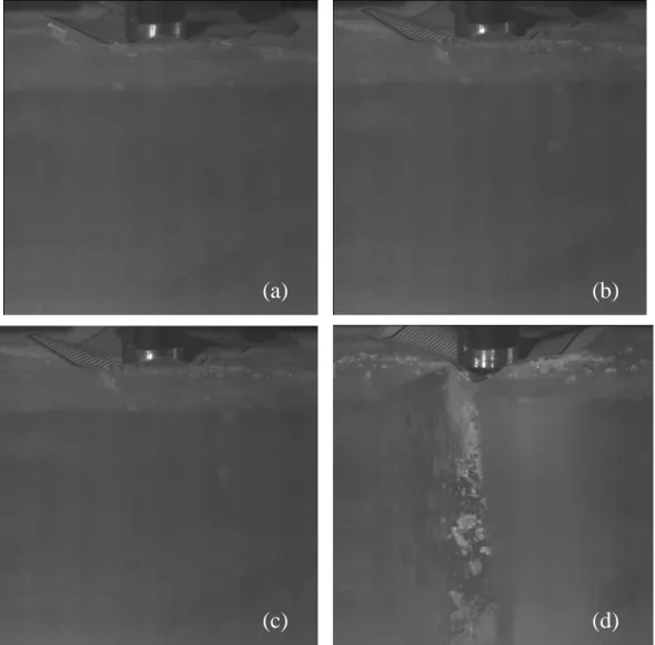
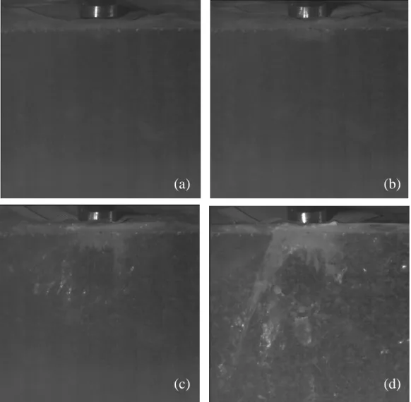
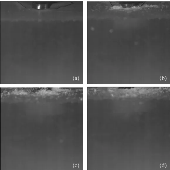
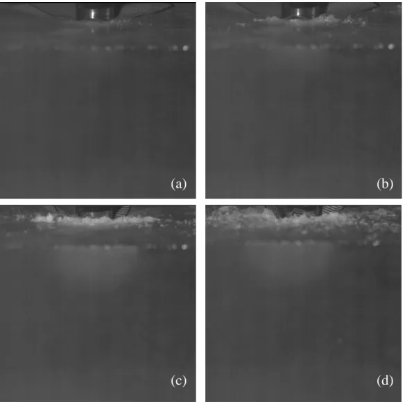
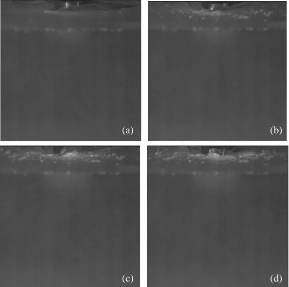
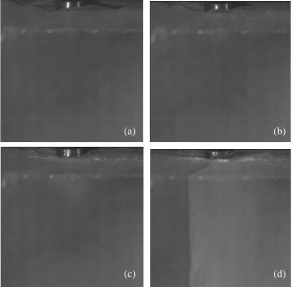
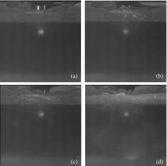
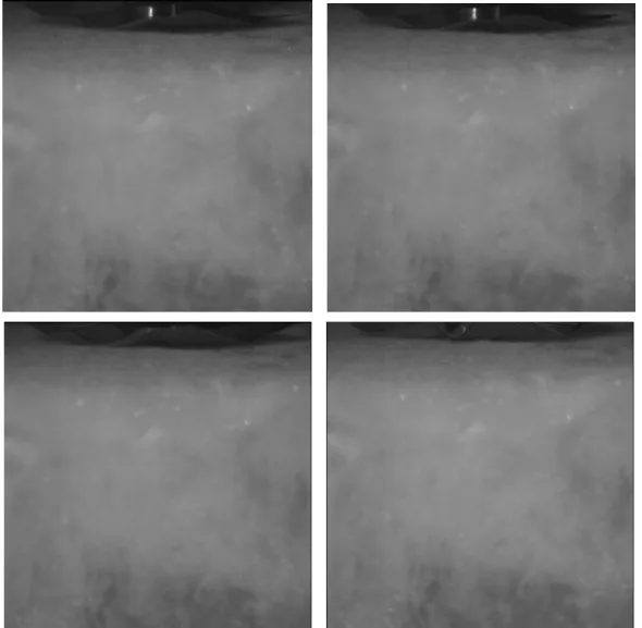
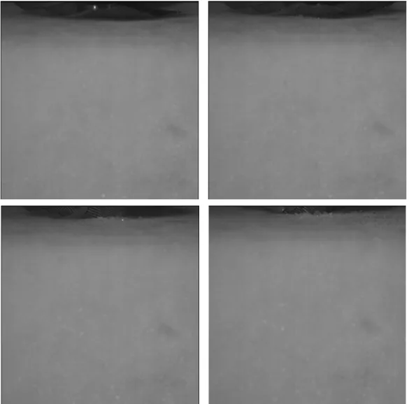
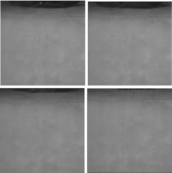
Information (CISTI). Appendix 3 includes a series of frames from each of the high-speed videos of the experiments. The figures show the formation and propagation of cracks a well as crushing and spalling behavior in the area of the indenter.

Similar to the test setup used in Phase I, an extremely bright, 532 nm, green laser pointer was used to provide additional illumination durin

d

the embedded crystal (Figures 4 and 5, Appendix 1). This light was then reflected by the many grain boundaries in the polycrystalline ice. The location of the monocrystal is visible since the lack of grain boundaries in this area produce a void in the sheet of ligh The intention of this sheet of light is to provide evidence for the fracture being

precipitated by the large grain boundary. Any fractures that begin inside the sample in the area of the crystal should reflect this light more strongly th

b

Synchronization between the data collected b v

the beginning of each test. This pulse simultaneously triggered both the initiation of the indenter and the initiation of the high-speed video.

(20)

is no ink. Measurements were taken by recording the changes in current flow at each sensel giving the applied force distribution. Using the I-Scan system, it is possible to record the force distribution at a rate of up to 100 frames per second. The pressure distribution is then calculated using the applied force and total contact area for e The pressure sensitive film used in these tests had a pressure rating of 25,000 PSI. During these tests, the pressure sensor was placed between the indenter and the surface the ice. The calibration of the sensor is described in Appendix 8.

ach time.

of

.0 POST-TEST THIN SECTIONS

hin-sectioning of the indentation site of selected tested specimens was performed

ture

elded to e free surface and the first slide was removed using a small blade. The new free surface

s,

inally, the thin sections were photographed under cross-polarized light to facilitate easy

e

ppendix 5, Figures 145–181 shows time histories of the total force that were recorded d by the load cell is

5

T

approximately one week after testing. Thin sections were taken parallel to the axis of indentation. When fracture occurred, the sections were taken perpendicular to the frac plane. The thin-sectioning was done using the “Double Microtome” technique introduced by Sinha (1977). First, a section of ice approximately 5–6 cm thick was welded onto a clean glass slide using a bead of water along three sides, avoiding the indentation area. A microtome blade was used to “shave” samples of ice from the free surface until a desired thickness was reached. A second glass slide was then w

th

was again microtomed, this time to 0.5–1.0 mm in thickness, thus allowing the crystal structure of the ice to be examined (Figure 3(a), Appendix 1). It should be noted that typically a thin section would be welded to the glass slide by a bead of water around the full perimeter of the sample. In our case however, the sample was only welded on 3 side leaving the side that was indented untouched.

F

viewing of the various crystals. The thin sections were also photographed under plain transmitted light with a side light oriented at approx 45 degrees to the sample (Figur 3 (b), Appendix 1). This side lighting was reflected by the crack surfaces highlighting any micro cracking that was present in the thin section. Photographs of the thin-sections, under both lighting conditions are included in Appendix 4.

6.0 EXPERIMENTAL RESULTS

A

(21)

analysi

include anual calibration of the pressure sensor. At the present time, a two-point calibration has been applied to the data given in this report (see appendix 8 for a detailed description of the two-point calibration). While this method is adequate for our application and is the one recommended by Tekscan, reduced uncertainty may be possible through the use of a manual calibration.

A closer look at the high-speed video should also give valuable information. First, it will be useful to determine whether the crack propagation begins in the area of the embedded monocrystal. Then, a comparison must be made between fluctuations in the load traces and visual events such as crushing, spalling and fracture. It would be helpful to write a program to manually synchronize the HSV, load cell data and pressure sensor to aid in this process.

Additionally, it will be of benefit to make a further comparison between these results and the results found in previous studies that do not include an embedded crystal. This comparison should focus not only on the effects of including the embedded crystal as a flaw, but also on the effects of including other flaws such as bubble density and varying ice composition. An effort should also be made to study how the cyclic loading behavior observed in some tests relates to failure processes and rate of indentation.

Finally, it will be necessary to address the sources of error that were present in the current test series. These sources of error include:

• Variation in average grain size of polycrystalline ice. • Variation in dimensions and placement of monocrystal. • Physical dimensions and surface finishing of ice specimen.

A great deal of work still remains in the analysis of the experimental data and as such, the s will be reported elsewhere. However, recommendations for analysis will be

(22)

8.0 REFERENCES

Barrette, P., J. Pond, C. Li and I. Jordaan. 2003. Laboratory-scale indentation of ice. PERD/CHC Report 4-81.

Mackey, T.R. 2006. Laboratory indentation testing of polycrystalline ice: An

investigation of fracture. Master’s Thesis, Memorial University of

Newfoundland, Newfoundland, Canada.

Sinha, N.K. 1977. Technique for studying the structure of sea ice. Journal of

Glaciology, 18: 315-323.

Wells, J., I. Jordaan, A. Derradji-Aouat, and A. Bugden. 2007. Laboratory investigation of the fracture behavior of polycrystalline ice with embedded monocrystals – Phase I. NRC Technical Report, January 2007.

(23)

(24)

APPENDIX 1: TEST PARAMETERS AND SAMPLE PREPARATION Table 1. Labels and information for each test.

Group Label Test Te Penetration

# Ice Type Test # ) 1 39 center 2 40 center 17 55 center 4 42 center 5 43 intermediate 6 44 intermediate 7 45 intermediate 8 46 intermediate 9 47 center vertical 10 48 intermediate vertical 11 49 center vertical 12 50 center vertical 13 51 center vertical 14 52 intermediate vertical 15 53 intermediate vertical 16 54 intermediate vertical 3 41 center 10 18 56 center 6 19 57 center 20 58 center 5 21 59 center 5 22 60 center 5 23 61 center 4 24 62 center 3 25 63 center 3 26 64 center 3 27 65 center 6 28 66 center 3 29 67 center 30 68 center 31 69 center 32 70 center 33 71 center ystalline m with ystalline mm talline m edded crystal lpter N/A N/A N/A 10 20 20 10 10 # Speed (mm/s) Loc st ation Crystal orientation Depth (in mm 2 2 10 10 2 2 10 10 10 c-axis 2 basal 10 basal 10 c-axis 10 basal 0.2 c-axis 2 c-axis 0.2 basal 10 4 4 6 4 4 4 5 5 3 3 10 8 2 10 2 0.2 2 Polycr ~ 4 m 4 3 Polycr 1 ~ 4 m 2 mono ~ 4 Polycrys Emb scu

(25)

5 43 -10.103 -4.41 - 6 44 -9.846 -4.27 - 7 45 -9.775 -3.39 - 8 46 -10.0 0 8 -3.65 - 9 47 -10.074 -3.50 - 10 48 -9.818 -3.80 - 11 49 -10.117 -4.96 - 12 50 -10.178 -4.58 - 13 51 -10.063 -4.09 - 14 52 -10.255 -4.06 - 15 53 -10.310 -3.97 - 16 54 -10.055 -2.99 - 3 41 -9.972 -4.34 - 18 56 -10.176 -4.10 - 19 57 -9.957 -4.08 914 20 58 -9.548 -2.70 - 21 59 -10.131 -3.40 - 22 60 -10.121 -3.73 - 23 61 -10.263 -3.86 - 24 62 -10.300 -3.91 - 25 63 -10.015 -4.10 - 26 64 -10.055 -4.13 - 27 65 -10.183 -4.02 - 28 66 -10.138 -3.87 - 29 67 -10.158 -5.28 907 30 68 -10.010 - 913 31 69 -9.870 -4.56 - 32 70 -9.885 -4.04 - 33 71 -9.566 -3.52 - 34 72 -9.321 -3.30 -

(26)

tem Figure 1. (a) MTS located at the NRC-IOT (b) Tekscan I-Scan pressure sensor system that was used to provide the pressure distributions for each test. The sys consists of a thin, flexible pressure sensing film that is connected to a computer outside of the testing area via a data handle with a USB connection.

(27)

Figure 3. (a) microtome used in the production of the post-test thin sections. (b) Light table used in the photography of the thin sections. In order to view he

e light source.

t sections under cross polarized light, the sections are placed between two filters which are located on the top two levels of the light table. Reflected light photos ar taken by placing the section on the top of the light table and adding light from an additional

(28)

Figure 5. Photograph taken prior to test I06_V2P0_I_025 that shows how the vertical sheet of laser light can be used to illustrate the position of the embedded monocrystal. The crystal can be seen as a void in the light, directly underneath the indenter.

(29)

(30)

APPENDIX 2: INDENTER DISPLACEMENT

(31)

(32)

(33)

(34)

(35)

(36)

(37)

(38)

(39)

(40)

(41)

(42)

(43)

(44)

(45)

(46)

(47)

(48)

(49)

(50)

APPENDIX 3: HIGH-SPEED VIDEO STILLS AND POST-TEST PHOTOGRAPHS

Figure 43. Sequence of frames taken from the high-speed video of I07_V2P0_C_039 a) t = 0.40 s (b) t = 1.68 s (c) t = 2.05 s (d) t = 2.73 s

(a)

(b)

(d)

(c)

(51)

Figure 44. Sequence of frames taken from the high-speed video of I (a) t = 0.93 s (b) t = 1.64 s (c) t = 2.27 s (d) t = 2.73 s

07_V2P0_C_040

(b

(a)

)

(52)

(a)

(b)

(c)

(d)

Figure 45. Sequence of frames taken from the high-speed video of I07_V10P0_C_041 (a) t = 0.15 s (b) t = 0.45 s (c) t = 0.69 s (d) t = 0.87 s

(53)

(a)

(b)

(54)

Figure 47. Sequence of frames taken from the high-speed video of I07_V2P0_I_043 (a) t = 0.26 s (b) t = 0.90 s (c) t = 1.29 s (d) t = 1.71 s

(55)

(a

(b

(c

(d

)

(56)

(a)

(b)

(57)

Figure 50. Sequence of frames taken from the high-speed video of I (a) t = 0.11 s (b) t = 0.24 s (c) t = 0.27 s

07_V10P0_I_046

(c)

(58)

(a)

(d

(65)

(a)

(b)

the high-speed video of I07_V3P0_C_064 Figure 68. Sequence of frames taken from

(a) t = 0.29 s (b) t = 0.45 s (c) t = 0.77 s (d) t = 1.04 s

(a)

(b)

(76)

igure 69. Sequence of frames taken from the high-speed video of ) t = 0.26 s (c) t = 0.35 s (d) t = 0.50 s

)

(b)

(80)

(a)

(c)

(d)

(81)

(a)

(b)

(c)

(d)

(82)

(83)

(84)

(85)

(86)

(87)

(88)

(89)

(90)

(91)

Figure 88. Experimental stills taken immediately after testing of I07_EMC_V10P0_C_047

(92)

Figure 90. Experimental stills taken immediately after testing of I07_EMB_V10P0_C_049

(93)

Figure 92. Experimental stills taken immediately after testing of I07_EMB_V10P0_C_051

(94)

Figure 94. Experimental stills taken immediately after testing of I07_EMC_V2P0_I_053

(95)

(96)

(97)

taken immediately after testing of I07_V4P0_C_059 Figure 100. Experimental stills

(98)

(99)

(100)

(101)

(102)

Figure 110. Experimental stills taken immediately after testing of I07_V2P0_C_069 (Specimen is mislabeled in photograph).

(103)

(104)

(105)

(106)

(107)

7_EMC_V10P0_C_047_A show

d lighting; (b) lighting; and (c) a combination of polarized and

side-Figure 118. Thin-sections from I0 n under (a)

polarize

(108)

(109)

(110)

(111)

(112)

(113)

(114)

(115)

igure 126. Thin-sections from I07_EMB_V10P0_C_051_A shown under (a) olarized lighting; (b) lighting; and (c) a combination of polarized and side-ghting conditions.

F p li

(116)

Figure 127. Thin-sections from I07_ n under (a)

polarize

lighting conditions.

EMB_V10P0_C_051_B show

(117)

(118)

(119)

(120)

(121)

igure 132. Thin-sections from I07_EMC_V2P0_I_053_A shown under (a)

ed lighting; (b) side-lighting. The indentation area was accidentally flooded with water prior to taking these photos.

F polariz

(122)

Figure 133. Thin-sections from I07_EMC_ n under (a) polarized lighting; (b) side-light

were taken and a thin-s

V2P0_I_053_B show

ing. The section was broken immediately after these photos ection was not obtained.

(123)

Figure 134. Thin-sections from I07_EMC_V2P0_I_053_C shown under (a) polarized lighting; (b) lighting; and (c) a combination of polarized and side-lighting conditions.

(124)

(125)

(126)

(127)

(128)

Figure 139. Thin-sections from I07_V3P0_C_064 shown under (a) polarized lighting; (b) side-lighting; and (c) a combination of polarized and side-lighting conditions.

(129)

Figure 140. Thin-sections from I07_V2 n under (a) polarized lighting; (b) side-light

conditions.

P0_C_067_A show

(130)

(131)

(132)

ig gh on

F ure 143. Thin-sections from I07_V0P2_C_070_B shown under (a) polarized ting; (b) side-lighting; and (c) a combination of polarized and side-lighting ditions.

li c

(133)

(134)

APPENDIX 5: LOAD TRACES

(135)

(136)

(137)

(138)

(139)

(140)

(141)

(142)

(143)

(144)

(145)

(146)

(147)

(148)

(149)

(150)

(151)

(152)

(153)

(154)

APPENDIX 6: MEAN NOMINAL STRESS

Figure 182. Diagram showing the calculation of the nominal / projected area of the spherical indenter.. The nominal area represents the area of a circle that has a radius that changes according to the depth of penetration of the indenter.

(155)

(156)

(157)

(158)

(159)

Figure 191. Mean Nominal Stress as a function of time for test I07_EMC_V10P0_C_047

(160)

Figure 193. Mean Nominal Stress as a function of time for test I07_EMB_V10P0_C_049

(161)

Figure 195. Mean Nominal Stress as a function of time for test I07_EMB_V10P0_C_051

(162)

Figure 197. Mean Nominal Stress as a function of time for test I07_EMC_V2P0_I_053

(163)

(164)

(165)

(166)

(167)

(168)

(169)

(170)

(171)

(172)

(173)

(174)

APPENDIX 7: PRESSURE SENSOR DATA

Figure 220. Maximum pressure and average pressure as a function of time for test I07_V2P0_C_039

(175)

(176)

Figure 224. Maximum pressure and average pressure as a function of time for test I07_V2P0_I_043

(177)

Figure 226. Maximum pressure and average pressure as a function of time for test I07_V10P0_I_045

(178)

Figure 228. Maximum pressure and average pressure as a function of time for test I07_EMC_V10P0_C_047

(179)

Figure 230. Maximum pressure and average pressure as a function of time for test I07_EMB_V10P0_C_049

(180)

Figure 232. Maximum pressure and average pressure as a function of time for test I07_EMB_V10P0_C_051

(181)

Figure 234. Maximum pressure and average pressure as a function of time for test I07_EMC_V2P0_I_053

(182)

(183)

(184)

(185)

(186)

(187)

(188)

(189)

(190)

(191)

(192)

(193)