Artificial Intelligence-Assisted Data Analysis with
BayesDB
by
Christina M. Curlette
Submitted to the Department of Electrical Engineering and Computer
Science
in partial fulfillment of the requirements for the degree of
Master of Engineering in Electrical Engineering and Computer Science
at the
MASSACHUSETTS INSTITUTE OF TECHNOLOGY
September 2017
c
○ Massachusetts Institute of Technology 2017. All rights reserved.
Author . . . .
Department of Electrical Engineering and Computer Science
September 5, 2017
Certified by . . . .
Vikash K. Mansinghka
Research Scientist
Thesis Supervisor
Accepted by . . . .
Christopher Terman
Chairman, Department Committee on Graduate Theses
Artificial Intelligence-Assisted Data Analysis with BayesDB
by
Christina M. Curlette
Submitted to the Department of Electrical Engineering and Computer Science on September 5, 2017, in partial fulfillment of the
requirements for the degree of
Master of Engineering in Electrical Engineering and Computer Science
Abstract
When applying machine learning and statistics techniques to real-world datasets, problems often arise due to missing data or errors from black-box predictive models that are difficult to understand or explain in terms of the model’s inputs. This thesis explores the applicability of BayesDB, a probabilistic programming platform for data analysis, to three common problems in data analysis: (i) modeling patterns of missing data, (ii) imputing missing values in datasets, and (iii) characterizing the error behavior of predictive models. Experiments show that CrossCat, the default model discovery mechanism used by BayesDB, can address all three problems effectively. Examples are drawn from the American National Election Studies and the Gapminder database of global macroeconomic and public health indicators.
Thesis Supervisor: Vikash K. Mansinghka Title: Research Scientist
Acknowledgments
First, I would like to thank my advisor, Vikash Mansinghka, for his excellent guidance, feedback, and mentorship throughout the M.Eng. program. I am especially grateful to my parents, Bill and Cathy Curlette, for their support and encouragement. I would like to thank Feras Saad for his helpful guidance and feedback on much of the work that has gone into this thesis as well as the thesis itself, and I would like to thank Ulrich Schaechtle for his help with the section on modeling errors of predictors. I would also like to thank Marco Cusumano-Towner, Taylor Campbell, Alexey Radul, Amanda Brower, and Veronica Weiner. Finally, I am grateful to DARPA for funding this research and my appointment as a research assistant through the Probabilistic Programming for Advancing Machine Learning program.
Contents
1 Introduction 13
1.1 Background: BayesDB . . . 14
1.2 Notation and definitions . . . 15
2 Modeling patterns of missing data 17 2.1 Missing data mechanisms . . . 18
2.2 Motivation for modeling patterns of missing data . . . 18
2.3 Modeling missing data with BayesDB . . . 20
2.4 Discussion and future work . . . 21
3 Imputing missing values 29 3.1 Motivation for imputation . . . 29
3.2 CrossCat imputation algorithm for nominal data . . . 30
3.3 Nominal imputation using BayesDB . . . 31
3.3.1 Subsampling the data . . . 32
3.3.2 Imputation methods and results . . . 32
3.4 Discussion and future work . . . 33
4 Modeling errors of predictors 39 4.1 Motivation for error monitoring . . . 40
4.2 Generative monitoring model framework . . . 40
4.3 Generative monitoring models using BayesDB . . . 42
4.3.2 Monitoring a nominal prediction . . . 52 4.4 Discussion and future work . . . 57
List of Figures
2-1 SQL and BQL code for adding missingness indicators. . . 24
2-2 Probable dependencies among missingness indicators and inputs. . . . 25
3-1 BQL and MML code for ANES imputations. . . 35
3-2 ANES imputation calibration lines. . . 36
3-3 ANES imputation accuracy. . . 37
4-1 Reliability analysis with probabilistic programming. . . 41
4-2 Predictive model and monitoring model with MML and BQL (Gapminder). 46 4-3 BQL for Gapminder monitor dependence probability heatmap. . . 47
4-4 Dependence of error pattern on input features (Gapminder). . . 48
4-5 Simulating error pattern. . . 49
4-6 Comparing similarity in the context of error pattern. . . 50
4-7 Simulating error pattern conditioned on other variables (Gapminder). 51 4-8 Predictive model and monitoring model with MML and BQL (ANES). 55 4-9 Dependence of error pattern on input features (ANES). . . 59
4-10 Mutual information of error pattern with an input variable. . . 60
4-11 Simulating error pattern conditioned on other inputs (ANES). . . 61
4-12 Simulating inputs conditioned on error pattern. . . 62 4-13 Simulating inputs conditioned on error pattern and additional inputs. 63
List of Tables
2.1 Sample of Gapminder data. . . 23
2.2 Values of probably dependent missingness indicators. . . 26
2.3 Prediction accuracy with and without missingness model. . . 27
3.1 ANES imputation calibration statistics. . . 37
4.1 Variables and statistical types of variables in the Gapminder population. 44 4.2 Variables and statistical types of variables in the Gapminder population (cont’d). . . 45
4.3 Variables and statistical types of variables in the ANES 2016 population. 53 4.4 Variables and statistical types of variables in the ANES 2016 population (cont’d). . . 54
Chapter 1
Introduction
When applying machine learning and statistics techniques to real-world datasets, problems often arise due to missing data or errors from black-box predictive models that are difficult to understand or explain in terms of the model’s inputs. This thesis shows how to use BayesDB, a probabilistic programming platform for data analysis, backed by CrossCat, a domain-general, nonparametric Bayesian modeling method, to (i) model patterns of missing data, (ii) impute missing values, and (iii) model errors of predictors, using examples from real-world datasets. This thesis illustrates how to formulate these problems in BayesDB using its built-in Bayesian Query Language (BQL) and Meta-Modeling Language (MML), thus demonstrating BayesDB’s flexibility as a tool for addressing common problems in data science. Advantages of using probabilistic methods to address handling missing data and modeling errors of black-box predictors are discussed, and empirical results are provided that support BayesDB’s effectiveness and accuracy at these tasks. Underlying all of these BayesDB workflows is CrossCat’s automatic data modeling capability, which infers models of full joint distributions of multivariate data without requiring users to hand-tune parameters. Automatic modeling serves as a form of artificial intelligence for data science and machine learning tasks, including the ones that this thesis focuses on. The approaches introduced in this thesis integrate seamlessly with established exploratory data analysis workflows using BayesDB. A more detailed description of BayesDB can be found in Section 1.1 and in Mansinghka et al. (2015). A full description of CrossCat can be found in
Mansinghka et al. (2016).
1.1
Background: BayesDB
BayesDB is a probabilistic programming platform for data science that enables rapid data modeling and analysis with few lines of code (Mansinghka et al., 2015). BayesDB’s core functionalities often make it possible for domain experts to answer questions in seconds or minutes that would otherwise require hours or days of work by someone with good statistical judgment (MIT Probabilistic Computing Project, b). BayesDB has two built-in languages: Bayesian Query Language (BQL) and Meta-Modeling Language (MML). The versions of BQL and MML referenced in this paper were written as extensions to SQLite.
MML is used to build populations from data tables by mapping columns in the tables to statistical types, such as numerical or nominal. A variable’s statistical type specifies its model type, e.g. normal, multinomial, etc. MML is also used to build analyses for populations via analysis schemas, which specify modeling strategies for the variables in the population. The default modeling strategy in BayesDB is CrossCat, described in Mansinghka et al. (2016). CrossCat can be overridden for any subset of the variables by built-in models, such as linear regression models or random forests, as well as custom models written in the VentureScript probabilistic programming language (Saad and Mansinghka, 2016).
BQL is used to create tables from files of comma-separated values (csv) and to query existing populations and analyses created using MML. BQL supports model estimation queries, such as estimating probability of dependence, mutual information, and correlation between variables, estimating predictive probability of observed or hypothetical values, and estimating predictive relevance between observed rows and observed or hypothetical rows. BQL also supports queries for simulating hypothetical data (including conditional simulation) and queries for inferring missing values. Full documentation of BQL and MML can be found online (MIT Probabilistic Computing Project, a).
Existing work on BayesDB has shown that it can successfully detect anomalous values and simulate plausible database records (Saad and Mansinghka, 2016). BayesDB has also been shown to be able to detect true predictive relationships that other methods often miss, while also suppressing false positives (Saad and Mansinghka, 2017). When applied to real-world datasets, BayesDB has been shown to find common sense dependencies among variables that match the ground truth in domains ranging from healthcare to politics (Mansinghka et al., 2016).
1.2
Notation and definitions
Throughout this paper, numerical is used as a descriptor for continuous-valued data. Nominal and categorical are used interchangeably as descriptors for discrete-valued data with finite, small numbers of distinct values.
MML refers to BayesDB’s Meta-Modeling Language. BQL refers to BayesDB’s Bayesian Query Language.
View refers to a group of columns clustered together by CrossCat. In the context of CrossCat, cluster refers to the “inner cluster” of rows within a particular view (Mansinghka et al., 2016).
Chapter 2
Modeling patterns of missing data
Real-world datasets often suffer from the problem of missing data due to causes ranging from faulty data entry to machine failures to subjects electing not to respond to survey questions. For example, a researcher may mistype a value, a sensor may break during an experiment, or a person may not respond to a question on a sensitive topic, such as mental health. When values are missing, they are frequently assumed to be missing at random and ignored in common data analysis methods. If they are not in fact missing at random, this assumption can lead to biased conclusions being drawn from analyses. In reality, data are commonly not missing completely at random. For example, extreme (but valid) temperature readings may be more likely to be missing than less extreme ones, or older people may be more likely to skip a particular survey question than younger people. Being able to identify whether data are not missing completely at random and, if so, being able to model the missingness mechanism, are important to building robust and accurate machine learning and statistical models. This chapter shows how BayesDB can be used to model patterns of missing data and detect whether data are likely to be missing at random using a dataset of global macroeconomic and public health indicators.
2.1
Missing data mechanisms
There are three main types of missingness data mechanisms in the literature: Miss-ing Completely at Random (MCAR), MissMiss-ing at Random (MAR), and MissMiss-ing Not at Random (MNAR) (Little and Rubin, 2014). In this chapter, missingness indi-cator is used to describe an indiindi-cator variable that is equal to 1 if a value of the corresponding variable is missing and 0 if it is present. Given a dataset with ob-served variables 𝑋, missingness indicators 𝑀 , and latent variables 𝑍, its full joint distribution can be defined as 𝑃 (𝑀 |𝑋, 𝑍, 𝜃1)𝑃 (𝑋, 𝑍|𝜃2), where 𝜃1 and 𝜃2 are
distri-butional parameters (Marlin, 2008). 𝑃 (𝑀 |𝑋, 𝑍, 𝜃1) is the missing data model, and
𝑃 (𝑋, 𝑍|𝜃2) is the non-missing data model. A variable 𝑥 is MCAR if its missingness
indicator, 𝑀𝑥, is independent of the values of 𝑥 itself, other variables, and latent
variables, i.e. 𝑃 (𝑀𝑥|𝑋, 𝑍, 𝜃1) = 𝑃 (𝑀𝑥|𝜃1) (Marlin, 2008). A variable 𝑥 is MAR if
its missingness indicator, 𝑀𝑥, depends only on observed values of other variables,
i.e. 𝑃 (𝑀𝑥|𝑋, 𝑍, 𝜃1) = 𝑃 (𝑀𝑥|𝑋𝑜𝑏𝑠, 𝜃1) where 𝑋𝑜𝑏𝑠 are variables’ observed values
(Marlin, 2008). MAR can be somewhat of a misleading term, because the data are systematically, rather than fully randomly, missing. A variable 𝑥 is MNAR if its missingness indicator, 𝑀𝑥, depends on the unobserved values of 𝑥 or unobserved values
of the latent variables. It may also depend on observed values of other variables, 𝑋𝑜𝑏𝑠 (Marlin, 2008). Intuitively, a variable is MNAR if the probability of observing its value depends on its own value or the value of an unmeasured latent variable. A couple of common causes of MNAR data are survey nonresponse and subjects dropping out of longitudinal studies (Marlin et al., 2005). Determining whether data are truly MNAR is very difficult — usually, it requires collecting more data about the missing values, e.g. through survey follow-up questions.
2.2
Motivation for modeling patterns of missing data
With the increasing prevalence of artificial intelligence systems, real-world data are playing an important role in decision-making technologies, from clinical decision
support to autonomous driving to personal assistants. However, the data sources used to train such systems likely have some missing values. Knowing the data missingness mechanism(s) can be used to improve the data collection process, determine which statistical tests and imputation methods are valid for a dataset, and improve prediction accuracy. In some cases, modifying the data collection process may elimininate or reduce the occurrence of missing values, and a model of the missingness patterns can help to inform how one might approach the problem. For example, if two quantities are being measured by the same sensor, and the quantities have interrelated patterns of missingness, one may want to use a separate sensor to measure each quantity in order to decouple them. Finding missingness indicators that are dependent on other recorded variables could also alert researchers to potential systematic flaws in collecting or recording data.
A typical workflow for handling missing data includes imputing the missing values. Unless a variable is MCAR, any imputation method that makes use of only information about that variable (e.g. mean imputation) is subject to bias. Little (1988) describes a general test for determining whether a dataset is MCAR. If there is evidence that a variable is MAR, then any other variable that its missingness is dependent on should be included in the imputation model. Logistic regression for modeling missingness indicators given the other variables in the dataset is one way to determine whether there is evidence that the data are MAR (Gelman). When it comes to imputation methods, regression models, random forest models, likelihood-based methods, and multiple imputation methods are valid whether the data are MCAR or MAR (Scheffer, 2002). On the other hand, MNAR data can lead to biased results in all of the aforementioned imputation schemes. However, some work has been done toward building unsupervised learning models that can handle MNAR data (Marlin, 2008; Marlin et al., 2005). Notably, incorporating explicit missingness models into machine learning models can also improve prediction accuracy (Marlin, 2008).
2.3
Modeling missing data with BayesDB
This section provides an example of using BayesDB to model patterns of missing data using a subset of data from the Gapminder Foundation containing social, political, economic, and geographic data for several countries in 2010 (Dietterich et al., 2017). The variables in the dataset are described in Table 3.2 (only a subset are used in this section). Table 2.1 shows a few representative entries in the dataset, all of which have several missing values. For each variable in the dataset, a missingness indicator was added. Figure 2-1 shows the SQL and BQL code for augmenting the dataset with missingness indicators.
Because CrossCat learns a full joint distribution over all the variables and missing-ness indicators, it models the missingmissing-ness mechanisms along with the data generating process. This section focuses on using BayesDB to distinguish MCAR and MAR pat-terns of missingness (ignoring MNAR, as it is impossible to directly detect). BayesDB can detect probable dependencies between data variables and missingness indicators, which provide information about whether variables are MCAR. If a variable is MCAR, its missingness indicator should fall into a view with at most its corresponding variable and possibly also other missingness indicators, thus indicating zero dependence proba-bility with any other variables. If a variable is MAR, its missingness indicator should fall into a view with variables other than the corresponding one and possibly also other missingness indicators. Figure 2-2 shows the probable dependencies between missingness indicators and variables for the Gapminder dataset. From the cluster structure in the heatmap, it is clear that some variables are likely to be MCAR, while others are more likely to be MAR. Table 2.2 provides a snapshot of some of the values of two missingness indicators that are found to be likely interdependent, which suggests that the corresponding variables are probably not MCAR.
In addition to detecting whether data are missing at random, BayesDB also provides at least a partial model of the underlying missing data mechanisms. This can be used to produce more accurate, less biased predictions. If a variable is MAR, the corresponding missingness indicator, other variables, and/or other missingness indicators may be
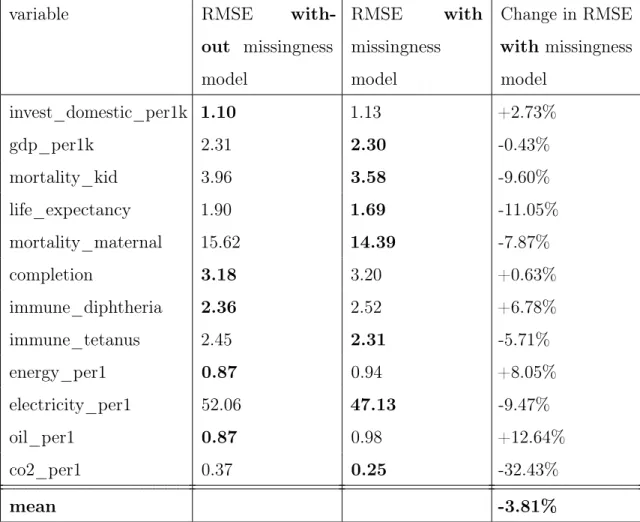
informative of it. Table 2.3 shows the root mean squared error (RMSE) of imputations of 30 randomly chosen censored values for each of several variables in the Gapminder data, both with and without including missingness indicators in the model. The variables were selected such that they had at least 50 percent probability of dependence on at least one other variable’s missingness indicator, so that the presence or absence of missingness indicators should affect accuracy. In both cases, 25 CrossCat models were trained with 1,000 iterations of analysis on all data excluding the censored values. Imputations were taken as the mean of 30 samples from the CrossCat models. In the majority of cases evaluated, including the missingness indicators improved the prediction accuracy. On average, adding missingness indicators reduced the RMSE by approximately 4 percent from the models without missingness indicators, also shown in Table 2.3. These results suggest that, in the case of MAR patterns, jointly modeling dummy variables for missingness with the rest of the variables can improve prediction accuracy.
2.4
Discussion and future work
In sum, categorizing and modeling patterns of missingness in datasets can aid in gaining a better qualitative understanding of the data, selecting appropriate statistical methods, and building more accurate predictors. This chapter has shown how to add missingness indicators to a real-world dataset with numerous missing values and model the missingness indicators alongside the input covariates using BayesDB. It has also shown how dependence probability estimates from CrossCat models can serve as indicators of systematic relationships between missingness indicators and other variables or other missingness indicators. Unlike regression models used to discover these relationships, BayesDB is well-suited to capture causal patterns, only requires one model for the whole dataset rather than a single model per variable, and is robust to missing values in the input data. Future work includes using BayesDB to model patterns of missingness in more datasets and comparing prediction accuracy with and without missingness indicators to other baselines. Another avenue for future work is
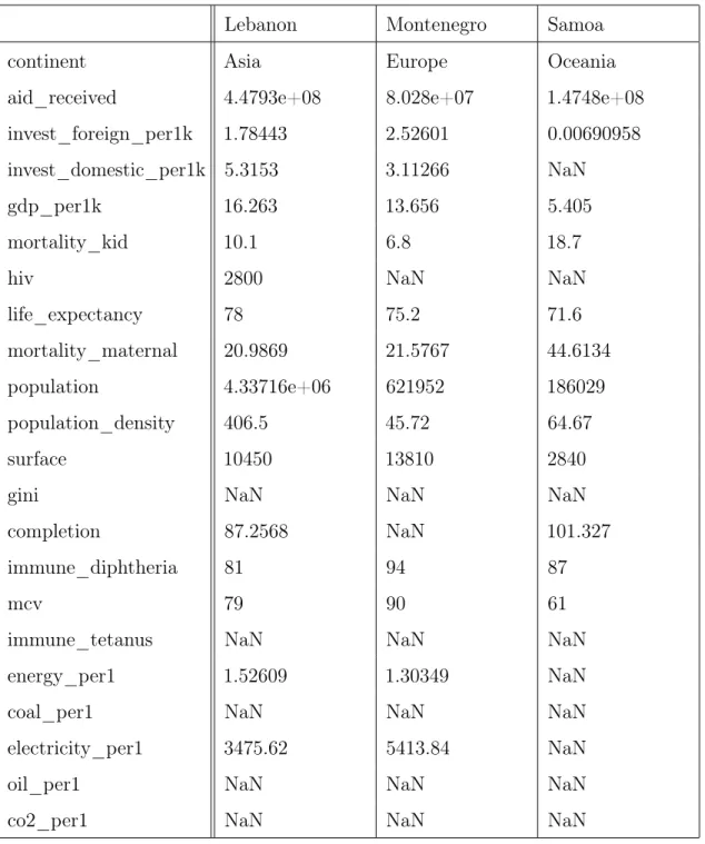
Table 2.1: Sample of Gapminder data. Data, including missing values, for three countries in the Gapminder dataset.
Lebanon Montenegro Samoa
continent Asia Europe Oceania
aid_received 4.4793e+08 8.028e+07 1.4748e+08
invest_foreign_per1k 1.78443 2.52601 0.00690958
invest_domestic_per1k 5.3153 3.11266 NaN
gdp_per1k 16.263 13.656 5.405
mortality_kid 10.1 6.8 18.7
hiv 2800 NaN NaN
life_expectancy 78 75.2 71.6
mortality_maternal 20.9869 21.5767 44.6134
population 4.33716e+06 621952 186029
population_density 406.5 45.72 64.67
surface 10450 13810 2840
gini NaN NaN NaN
completion 87.2568 NaN 101.327
immune_diphtheria 81 94 87
mcv 79 90 61
immune_tetanus NaN NaN NaN
energy_per1 1.52609 1.30349 NaN
coal_per1 NaN NaN NaN
electricity_per1 3475.62 5413.84 NaN
oil_per1 NaN NaN NaN
%%sql
CREATE TABLE missingness_indicators AS SELECT
CASE WHEN "country_id" IS NULL THEN 1 ELSE 0 END AS "missing_country_id", CASE WHEN "country" IS NULL THEN 1 ELSE 0 END AS "missing_country", CASE WHEN "continent" IS NULL THEN 1 ELSE 0 END AS "missing_continent", CASE WHEN "year" IS NULL THEN 1 ELSE 0 END AS "missing_year", CASE WHEN "aid_received" IS NULL THEN 1 ELSE 0 END AS "missing_aid_received", CASE WHEN "mortality_kid" IS NULL THEN 1 ELSE 0 END AS "missing_mortality_kid", CASE WHEN "life_expectancy" IS NULL THEN 1 ELSE 0 END AS "missing_life_expectancy", CASE WHEN "population" IS NULL THEN 1 ELSE 0 END AS "missing_population", CASE WHEN "population_density" IS NULL THEN 1 ELSE 0 END AS "missing_population_density", CASE WHEN "surface" IS NULL THEN 1 ELSE 0 END AS "missing_surface",
CASE WHEN "gini" IS NULL THEN 1 ELSE 0 END AS "missing_gini", CASE WHEN "hiv" IS NULL THEN 1 ELSE 0 END AS "missing_hiv",
CASE WHEN "professional_birth" IS NULL THEN 1 ELSE 0 END AS "missing_professional_birth", CASE WHEN "coal_per1" IS NULL THEN 1 ELSE 0 END AS "missing_coal_per1",
CASE WHEN "co2_per1" IS NULL THEN 1 ELSE 0 END AS "missing_co2_per1", CASE WHEN "oil_per1" IS NULL THEN 1 ELSE 0 END AS "missing_oil_per1", CASE WHEN "energy_per1" IS NULL THEN 1 ELSE 0 END AS "missing_energy_per1", CASE WHEN "electrictiy_per1" IS NULL THEN 1 ELSE 0 END AS "missing_electrictiy_per1", CASE WHEN "immune_diphtheria" IS NULL THEN 1 ELSE 0 END AS "missing_immune_diphtheria", CASE WHEN "mcv" IS NULL THEN 1 ELSE 0 END AS "missing_mcv",
CASE WHEN "immune_tetanus" IS NULL THEN 1 ELSE 0 END AS "missing_immune_tetanus" FROM gapminder_2010_t;
%%bql
CREATE TABLE gapminder_2010_with_missing_indicators_t AS SELECT * FROM missingness_indicators, gapminder_2010_t WHERE missingness_indicators.rowid = gapminder_2010_t.rowid;
Figure 2-1: SQL and BQL code for adding missingness
indica-tors. SQL code for creating a table of missingness indicators, called
missingness_indicators, and BQL code for combining it with the table of
raw data values, gapminder_2010_t. The result is an augmented table called
(a)
%%bql
.heatmap ESTIMATE DEPENDENCE PROBABILITY FROM PAIRWISE VARIABLES OF
gapminder_missingness; missing_oil_per1 missing_co2_per1 missing_coal_per1 electricity_per1 oil_per1 co2_per1 energy_per1 missing_immune_tetanus missing_aid_received gdp_per1k invest_domestic_per1k missing_mortality_kid mortality_kid life_expectancy completion continent immune_tetanus immune_diphtheria mcv mortality_maternal missing_invest_domestic_per1k missing_electricity_per1 missing_energy_per1 missing_hiv missing_invest_foreign_per1k missing_life_expectancy missing_surface missing_population_density missing_immune_diphtheria missing_mcv missing_gini missing_mortality_maternal invest_foreign_per1k population_density missing_completion population surface aid_received hiv coal_per1 gini missing_gdp_per1k missing_continent missing_population missing_oil_per1 missing_co2_per1 missing_coal_per1 electricity_per1 oil_per1 co2_per1 energy_per1 missing_immune_tetanus missing_aid_received gdp_per1k invest_domestic_per1k missing_mortality_kid mortality_kid life_expectancy completion continent immune_tetanus immune_diphtheria mcv mortality_maternal missing_invest_domestic_per1k missing_electricity_per1 missing_energy_per1 missing_hiv missing_invest_foreign_per1k missing_life_expectancy missing_surface missing_population_density missing_immune_diphtheria missing_mcv missing_gini missing_mortality_maternal
invest_foreign_per1k population_density missing_completion
population surface aid_received hiv coal_per1 gini
missing_gdp_per1k missing_continent missing_population
(b)
Figure 2-2: Probable dependencies among missingness indicators and inputs. (a) shows the BQL code for computing the probabilities of dependence between
variables and missingness indicators in the Gapminder data. (b) depicts the resulting heatmap. Variable names in red are missingness indicators. The clusters in the heatmap containing multiple missingness indicators and variables likely indicate MAR patterns of missingness. The clusters containing only individual missingness indicators suggest likely MCAR patterns of missingness.
Table 2.2: Values of probably dependent missingness indicators. A sam-ple of rows from the Gapminder dataset for two missingness indicator variables, missing_co2_per1 and missing_coal_per1, which have high probability of
de-pendence. Boldface font indicates that the values of missing_co2_per1 and
missing_coal_per1 are the same in that row. Coal_per1 and co2_per1 are of-ten either both missing or both not missing, suggesting a systematic pattern of missingness of two variables that may relate to their underlying values.
country missing_co2_per1 missing_coal_per1
Sudan 1.0 1.0 Cote d’Ivoire 1.0 1.0 Syria 1.0 1.0 Nepal 1.0 1.0 Benin 1.0 1.0 Togo 1.0 1.0 Iran 0.0 0.0 Mauritius 1.0 1.0 Turkmenistan 1.0 0.0 Kuwait 1.0 0.0 Jamaica 1.0 1.0 Argentina 0.0 0.0 Tajikistan 1.0 1.0
Trinidad and Tobago 1.0 0.0
United States 0.0 0.0
Table 2.3: Prediction accuracy with and without missingness model. Root mean squared error (RMSE) of CrossCat imputations of 30 held-out values per variable both with and without modeling missingness indicators. The variables were selected such that they were at least 50 percent likely to be dependent on at least one other variable’s missingness indicator. The values in bold indicate the lower RMSE for each variable. The model with missingness indicators had lower RMSE in most cases, and on average resulted in a decrease in RMSE from the model without missingness indicators.
variable RMSE
with-out missingness model RMSE with missingness model Change in RMSE with missingness model invest_domestic_per1k 1.10 1.13 +2.73% gdp_per1k 2.31 2.30 -0.43% mortality_kid 3.96 3.58 -9.60% life_expectancy 1.90 1.69 -11.05% mortality_maternal 15.62 14.39 -7.87% completion 3.18 3.20 +0.63% immune_diphtheria 2.36 2.52 +6.78% immune_tetanus 2.45 2.31 -5.71% energy_per1 0.87 0.94 +8.05% electricity_per1 52.06 47.13 -9.47% oil_per1 0.87 0.98 +12.64% co2_per1 0.37 0.25 -32.43% mean -3.81%
Chapter 3
Imputing missing values
Nowadays, large datasets are becoming increasingly important in solving problems across myriad domains, from economics to medicine to education. However, many real-world datasets are sparse, with missing values accounting for significant percentages of the data. Consequently, finding robust methods to impute missing values is critical. Some basic imputation techniques include imputing the mode, median, or mean value from the column or from a stratified sample of the population. Other more sophisticated techniques include using machine learning predictors, likelihood models, or multiple imputation methods to predict the missing values. This chapter describes a nonparametric Bayesian approach to imputation using CrossCat via the BayesDB interface. CrossCat provides a scalable sampling algorithm that can be used to impute missing values. This chapter presents empirical results showing that CrossCat is better calibrated and at least as accurate as other baselines for imputing nominal values in a dataset of individuals’ political views and engagement.
3.1
Motivation for imputation
In data analysis, missing data are commonplace and how they are handled can impact the conclusions drawn from analyses. One way to deal with missing data is complete case analysis, in which any row in the table with a missing value is simply deleted from the dataset. However, deleting rows from the data can reduce the power of
subsequent analyses by decreasing the sample size. Furthermore, unless the data are missing at random, removal of rows with missing values can also introduce bias, because the remaining rows may differ systematically from the original sample (Little and Rubin, 2014). Imputation methods address these problems by filling in missing values using information from the rest of the dataset, thus making all cases complete. Many types of imputation methods have been devised over the years, including regression-based methods, random forest-based models, multiple imputation schemes, and likelihood-based approaches (Little and Rubin, 2014; Stekhoven and Bühlmann, 2011). Imputation methods fall into two main categories: single imputation and multiple imputation. This chapter focuses on using CrossCat and other baselines for single imputation. Single imputation methods produce one complete dataset with a single prediction for each missing value. Ideally, each imputed value also has an associated confidence. In single imputation, the goal is to fill in missing values such that they match the true data as closely as possible. In general, when imputing missing values, it is important that the imputations are both accurate and well-calibrated, i.e., the average confidence of imputed values for a variable equals the average accuracy of the imputed values. In other words, the model assigns reasonable uncertainty to its imputations.
3.2
CrossCat imputation algorithm for nominal data
CrossCat simulations can be used to impute missing values of both nominal and numerical data. This chapter focuses on the case of nominal data. For nominal data, the imputed value from a set of 𝑛 simulated values 𝑠 = (𝑠1, . . . , 𝑠𝑛) is mode(𝑠). The
associated confidence of the imputation is 1𝑛∑︀𝑛
𝑖=1I[𝑠𝑖 = mode(𝑠)], where I is the
Algorithm 1 impute-nominal for CrossCat (Mansinghka et al., 2015).
function impute-nominal
𝑠(𝑟,𝑞)← ∅ ◁ initialize empty set of simulated values
𝑖 ← 0
while 𝑖 < 𝑛 do ◁ simulate 𝑛 values of 𝑞 for row 𝑟
𝑠 ← Simulate(𝑞) Given {𝑑𝑖 = 𝑥(𝑟,𝑑𝑖)} for 𝑑𝑖 ̸= 𝑞 ◁ simulate the value of 𝑞 given all
other values in row 𝑟
𝑠.append(𝑠) ◁ append 𝑠 to the set of simulated values
end while modeFreq ← 0
for 𝑠 ∈ 𝑠(𝑟,𝑞) do ◁ for each value 𝑠 in 𝑠(𝑟,𝑞)
if 𝑠 = mode(𝑠(𝑟,𝑞)) then ◁ if 𝑠 is equal to the mode of 𝑠(𝑟,𝑞)
modeFreq ← modeFreq + 1 ◁ increment modeFreq by 1
end if end for
conf ← modeFreq/𝑛 ◁ set conf to the proportion of values equal to the mode
return mode(𝑠(𝑟,𝑞)), conf ◁ imputed value and confidence
end function
Details of the Simulate algorithm can be found in Saad and Mansinghka (2016).
3.3
Nominal imputation using BayesDB
This experiment used a subset of data from the American National Election Study (ANES) 2012. The ANES dataset contains information about people’s voting patterns, opinions on issues, and political participation (American National Election Studies). The imputation task here is framed as a supervised prediction task, in which values are imputed for a set of held-out test cells whose true values are known.
3.3.1
Subsampling the data
The ANES dataset contains responses from nearly 6,000 people and more than 2,200 variables (mostly responses to survey questions). First, the variables were downsampled to a subset of 105 nominal variables relating to campaign interest and engagement; media exposure and attention; registration, turnout, and vote choice; likes and dislikes for major party presidential candidates; congressional approval; and presidential and status quo approval. Of the 105 variables, the 30 with the fewest missing values were selected for the prediction task. These variables had between 2 and 8 categories, with an average of 3.27.
700 rows were selected at random. This ensured there would be a sufficient number of rows with known values for training and test data. The final number of rows used for training and test data was chosen such that each of the 30 variables had at least that many known values. Each predictive model was trained on 340 rows and tested on 60 rows. The 400 total training and testing rows for each variable were randomly selected from the rows with known values for that variable in the 700-row subsample. Then for each variable, 60 of the 400 rows were randomly selected to use as test data.
3.3.2
Imputation methods and results
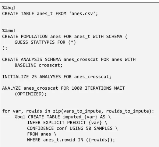
For each of the 30 variables, 25 CrossCat models were analyzed for 1,000 iterations. Values were then imputed for the 60 held-out test rows using the mode of 50 simulations from the CrossCat models. The associated confidence for each imputation was the percentage of simulated values equal to the mode simulated value. Figure 3-1 displays the BQL and MML code for performing these imputations.
For comparison, out-of-the-box random forest and logistic regression models were also applied to the same set of imputation tasks. The default Python scikit-learn implementations of random forest and logistic regression classifiers were used (Pe-dregosa et al., 2011). A separate classifier was trained for each variable to be imputed. For these models, the imputed value was the predicted class, and the associated confidence was the probability the model assigned to the predicted class. Missing
values (for variables other than the one to be imputed) were filled with the column median for numerical variables and the column mode for nominal variables. Imputing using the column mode for each variable was also included as a baseline; the associated confidence was how many values in the column were equal to the mode.
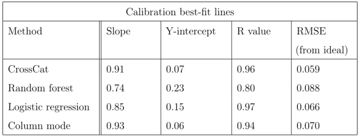
Figure 3-2 shows the calibration of imputations for CrossCat and other baselines, and Figure 3-3 compares their accuracy. Of the four methods, CrossCat was the most well-calibrated, with the lowest root mean squared error from the ideal calibration line. It was also on par with the accuracy of the logistic regression and random forest models and much more accurate than the column mode baseline, with an overall accuracy rate of 73 percent. These results suggest that CrossCat is better calibrated than other single imputation baseline methods without sacrificing accuracy.
3.4
Discussion and future work
Missing values, especially in real-world datasets, are commonplace. Thus, it is
important to have robust imputation strategies for practical data analysis tasks. This chapter has shown how to model sparse datasets and impute missing values using BayesDB. Empirical results on a dataset from the American National Election Studies provide preliminary evidence that CrossCat may be better calibrated and just as accurate as other methods for single imputation. It is worth noting that CrossCat is also more well-suited to handling missing data (for variables other than the one being imputed) when predicting missing values than baselines such as regression and random forest models. For example, while regression and random forests require missing data to be filled in in order to make a prediction, CrossCat does not. On the other hand, CrossCat is typically more computationally expensive than regression and random forest models, so there is a tradeoff between calibration and speed. Future work includes running nominal imputation experiments on additional datasets as well as comparing CrossCat to other single imputation baselines for numerical imputation. Another important area for future work is to use CrossCat as a multiple imputation scheme and compare it to methods such as Multiple Imputation by Chained Equations
%%bql
CREATE TABLE anes_t FROM ‘anes.csv’;
%%mml
CREATE POPULATION anes FOR anes_t WITH SCHEMA ( GUESS STATTYPES FOR (*)
);
CREATE ANALYSIS SCHEMA anes_crosscat FOR anes WITH BASELINE crosscat;
INITIALIZE 25 ANALYSES FOR anes_crosscat; ANALYZE anes_crosscat FOR 1000 ITERATIONS WAIT
(OPTIMIZED);
for var, rowids in zip(vars_to_impute, rowids_to_impute): %bql CREATE TABLE imputed_{var} AS \
INFER EXPLICIT PREDICT {var} \ CONFIDENCE conf USING 50 SAMPLES \ FROM anes \
WHERE anes_t.rowid IN ({rowids});
Figure 3-1: BQL and MML code for ANES imputations. The first %%bql block of code creates a table of the ANES data from a csv file. The %%mml code block creates a population for the table by mapping variables to heuristically guessed statistical types, and creates and analyzes CrossCat models for that population. The for-loop shows an example of code for imputing values using multiple samples from the CrossCat models.
0.0 0.2 0.4 0.6 0.8 1.0 Accuracy 0.0 0.2 0.4 0.6 0.8 1.0 Average confidence CrossCat calibration CrossCat Ideal (a) 0.0 0.2 0.4 0.6 0.8 1.0 Accuracy 0.0 0.2 0.4 0.6 0.8 1.0 Average confidence
Random forest calibration
Random forest Ideal (b) 0.0 0.2 0.4 0.6 0.8 1.0 Accuracy 0.0 0.2 0.4 0.6 0.8 1.0 Average confidence
Logistic regression calibration
Logistic regression Ideal (c) 0.0 0.2 0.4 0.6 0.8 1.0 Accuracy 0.0 0.2 0.4 0.6 0.8 1.0 Average confidence
Column mode calibration
Column mode Ideal
(d)
Figure 3-2: ANES imputation calibration lines. Calibration of CrossCat, random forest, logistic regression, and column mode imputations on ANES data. Each point represents one of the variables whose values were imputed. Each solid colored line is a regression line representing the model’s calibration, and each dotted black line represents ideal calibration. From the figure it is evident that CrossCat is better calibrated and about as accurate as the random forest and logistic regression models. It is also clear from the concentration of points around 0.9 accuracy for CrossCat and 0.6 for the column mode baseline that CrossCat is much more accurate than the column mode baseline.
Calibration best-fit lines
Method Slope Y-intercept R value RMSE
(from ideal)
CrossCat 0.91 0.07 0.96 0.059
Random forest 0.74 0.23 0.80 0.088
Logistic regression 0.85 0.15 0.97 0.066
Column mode 0.93 0.06 0.94 0.070
Table 3.1: ANES imputation calibration statistics. Slope, y-intercept, and r value of the calibration OLS regression line for four imputation methods applied to ANES data. The “RMSE (from ideal)” column displays the root mean squared error of the points from the ideal calibration line. CrossCat had the lowest RMSE of all methods.
CrossCat Random
forest regressionLogistic Column mode
Method 0.3 0.4 0.5 0.6 0.7 0.8 Accuracy
Average imputation accuracy
Figure 3-3: ANES imputation accuracy. Average accuracy of predictions made by CrossCat, a random forest, logistic regression, and the column mode on the same subset of data. CrossCat had similar accuracy as the logistic regression and random forest models, while also being better calibrated.
Chapter 4
Modeling errors of predictors
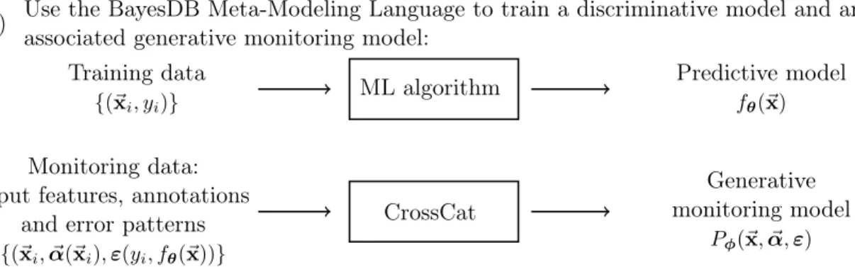
Machine learning algorithms produce predictive models whose patterns of error can be difficult to summarize and predict. Specific types of error may be non-uniformly distributed over the space of input features, and this space itself may be only sparsely and non-uniformly represented in the training data. This chapter shows how to use BayesDB to simultaneously (i) learn a discriminative model for a specific prediction of interest, and (ii) build a non-parametric Bayesian generative “monitoring model” that jointly models the input features and the probable errors of the discriminative model. Because it is hosted in a probabilistic programming system, the generative model can be interactively queried to (i) predict the pattern of error for held-out inputs, (ii) describe probable dependencies between the error pattern and the input features, and (iii) generate synthetic inputs that will probably cause the discriminative model to make specific errors. Unlike approaches based purely on optimizing error likelihood — including recently proposed approaches for finding “optical illusions” for neural nets (Nguyen et al., 2015)— the generative monitor also accounts for the typicality of the input under a generative model for the training data. This biases synthetic results towards plausible feature vectors. Figure 1 shows a schematic of the overall approach. This chapter illustrates these capabilities using the problems of predicting countries’ GDP and predicting U.S. citizens’ presidential votes.
4.1
Motivation for error monitoring
An autonomous system that makes predictions for self-driving cars or makes decisions in a medical context cannot function as a black box; rather, it needs to be explainable and reliable (e.g. Holdren and Smith, 2016; DARPA, 2016). Many recent research efforts aim to understand what impairs the reliability of machine learning systems and how they can be improved. Hand (2006) pointed out that some common assumptions made when using discriminative, predictive models render them unreliable. For example, training data is often not uniformly drawn from the distribution of the data that the predictive model will be applied to. Additionally, false certainty about the correctness of the training data’s labels can further lead to suboptimal performance. Sculley et al. (2014) explain such suboptimal performance as a kind of technical debt caused by a machine learning system’s dependence on training and test data. The authors describe the ability to monitor a machine learning system as “critical.” Some recent work has focused on building monitoring models for machine learning systems; for example, Ribeiro et al. (2016) introduced a monitoring system that infers explanations by observing and analyzing the input-output behavior of an arbitrary opaque predictive model.
4.2
Generative monitoring model framework
The approach in this chapter, outlined in Figure 4-1, makes use of probabilistic programming to jointly model input features and the types of errors made by discrim-inative black box machine learning models, which we call error pattern. We define error pattern as the output of a function of the true target value of an input and the predicted target value of an input. For numerical targets, error pattern could be, e.g., the residual or squared residual, and for nominal targets, error pattern could be a tuple of true class and predicted class or a Boolean value representing whether the predicted class is correct.
Training data
{(⃗x𝑖, 𝑦𝑖)}
ML algorithm Predictive model
𝑓𝜃(⃗x)
Use the BayesDB Meta-Modeling Language to train a discriminative model and an associated generative monitoring model:
(a)
CrossCat Monitoring data:
input features, annotations and error patterns
{(⃗x𝑖, ⃗𝛼(⃗x𝑖), 𝜀(𝑦𝑖, 𝑓𝜃(⃗x))}
Generative monitoring model
𝑃𝜑(⃗x, ⃗𝛼, 𝜀)
Query the generative monitoring model via the BayesDB Bayesian Query Language to summarize and predict error patterns of the discriminative model. Examples: (b)
Error pattern of interest𝜀*
Probable feature vectors and annotations
{︁⃗^x𝑗, ⃗^𝛼(︁⃗^x𝑗
)︁}︁
∼ 𝑃𝜑(⃗^x𝑗, ⃗^𝛼 | 𝜀 = 𝜀*)
Input features⃗x Probable error pattern
𝑃𝜑(𝜀 | ⃗x)
Query feature or annotation
x𝑑 or 𝛼𝑑
Probability of dependence with error pattern
𝑃𝜑[︀I (︀x𝑑; 𝜀)︀ > 𝛿]︀ or 𝑃𝜑[︀I (︀𝛼𝑑; 𝜀)︀ > 𝛿]︀ Generative monitoring model 𝑃𝜑(⃗x, ⃗𝛼, 𝜀) + BayesDB BQL implementation
Figure 4-1: Reliability analysis with probabilistic programming. (a) MML can be used to train a generative monitoring model. A generative monitoring model is a model for the joint distribution over input features, annotations, and error patterns. A black box machine learning (ML) algorithm is trained using a set of training data {(𝑥𝑖, 𝑦𝑖)}, resulting in a predictive model 𝑓𝜃(⃗x) where 𝜃 is a set of parameters for the
predictive model. Monitoring data consist of input features ⃗x, a potentially sparse auxiliary signal ⃗𝛼, and error pattern 𝜀 as a function of the model’s prediction and the true target. We model the generative monitor 𝑃𝜑(⃗x, ⃗𝛼, 𝜀) using CrossCat, where 𝜑
denotes the structure and parameters for CrossCat. (b) BQL can be used to query the generative monitoring model in order to explain error patterns, predict likely failures, and predict the likelihood that error pattern depends on other variables using mutual information; which above is written as I(x𝑑; 𝜀).
4.3
Generative monitoring models using BayesDB
This section demonstrates two examples of creating generative monitoring models for real-world datasets using BayesDB.
4.3.1
Monitoring a numerical prediction
This section makes use of data from the Gapminder Foundation. The Gapminder Foundation’s data comprise macroeconomic and public health indicators for countries around the world spanning the past few centuries. This example uses a subset of Gapminder data from 2010 containing 30 variables for 170 countries. A codebook for the subset of variables used in this example can be found in Tables 4.1 and 4.2, and a full codebook can be found online (Dietterich et al., 2017).
The variable gdp_per1k, a numerical variable, was modeled using ordinary least squares linear regression given the inputs continent, mortality_maternal,
population_density, aid_received, life_expectancy, and spending_health_per1. 100 rows of input data were used to fit the linear regression model, which was used to predict gdp_per1k for 70 held-out test rows. The error pattern in this case was residual, which was computed as (predicted gdp_per1k − true gdp_per1k) for the test rows. A monitoring model was then trained on the input covariates, predicted gdp_per1k, and residual. The monitoring model consisted of 25 CrossCat models analyzed for 1,000 iterations. Figure 4-2 displays the MML and BQL code used to construct and train the predictive and monitoring models. While linear regression is a relatively simple model, the approaches outlined in this section could be repeated using a more complex model, such as a deep neural network, to generate the predictions from which error pattern is derived.
Once the monitoring model has been trained, it can be queried for likely dependen-cies between error pattern and input covariates. Likelihood of dependence is defined as the probability that there exists nonzero mutual information between an input variable and the error pattern, in this case residual. Figure 4-3 shows the BQL code to obtain these dependence probabilities, and Figure 4-4 illustrates these dependency
relations in the Gapminder monitoring model.
One way to confirm that the monitoring model has indeed learned a satisfactory approximation of the distribution of error pattern is to compare the true distribution to a distribution of error patterns simulated from the monitoring model. Such a comparison can serve as a rough check of the quality of CrossCat’s model inference; substantial differences between the distributions can indicate that more iterations of analysis are needed. Figure 4-5 shows a comparison distributions of true GDP prediction residuals from the Gapminder monitoring data with residual values simulated from the monitoring model. The distributions appear quite similar, indicating that the generative monitoring model has learned an accurate model for the marginal distribution of GDP residuals.
The generative monitoring model can also be used to compute similarity of rows in the context of error pattern. Similarity is the probability over all CrossCat models that, within the view containing the error pattern variable, two rows are in the same cluster. Examining similarity of rows in the context of error pattern can reveal systemic differences in typical error for different types of inputs. Additionally, the clustering of rows based on similarity may expose a latent variable that is intuitive in light of domain knowledge. Such a variable may be further modeled by introducing it as a new column in the underlying table. For the Gapminder data, Figure 4-6 depicts the similarity between countries in the context of residual. In this case, CrossCat found systemic differences in residual across five main groups of countries. The clusters constitute intuitive groups with shared geographic and economic characteristics (e.g. New Zealand, US, Western Europe). These results were used to add a new country_cluster variable into the dataset and model it along with the original covariates. Results of GDP residual simulations conditional on different values of country_cluster are depicted in Figure 4-7. The distributions of residual simulations are noticeably different for the Africa country cluster compared to the US_West_Europe country cluster, indicating distinctive patterns of error for different types of countries.
Table 4.1: Variables and statistical types of variables in the Gapminder population.
Variable Description Statistical type
gdp_per1k GDP per 1000 people numerical
continent Continent where country is located nominal
gini GINI index numerical
professional_birth Births attended by trained staff numerical
electricity_per1 Electrical energy use per capita numerical
aid_received Total foreign aid received ($) numerical
surface Land area in square km numerical
invest_domestic_per1k Domestic investment per 1000 people numerical
population_density Population per square km numerical
immune_hepatitis HepB3 immunized (% of one-year-olds) numerical
spending_health_per1 Health spending per person ($) numerical
invest_foreign_per1k Foreign investment per 1000 people numerical
life_expectancy Life expectancy at birth numerical
water_source Proportion of population using
im-proved drinking water
numerical
hiv People living with HIV numerical
broadband Broadband subscribers per 100 people numerical
internet Internet users per 100 people numerical
mortality_maternal Maternal deaths per 100,000 live births numerical
coal_per1 Coal energy use per capita numerical
completion Primary school completion rate numerical
oil_per1 Oil consumption per capita numerical
co2_per1 CO2 emissions per capita numerical
mcv MCV immunized (% of one-year-olds) numerical
mortality_kid Child deaths before age 5 per 1,000 live
births
numerical
Table 4.2: Variables and statistical types of variables in the Gapminder population (cont’d).
Variable Description Statistical type
immune_tetanus PAB immunized (% of newborns) numerical
sanitation Proportion of population using
im-proved sanitation
numerical
immune_hib Hib3 immunized (% of one-year-olds) numerical
immune_diphtheria DTP3 immunized (% of one-year-olds) numerical
energy_per1 Energy consumption per capita numerical
(a) %%mml
CREATE POPULATION gapminder FOR gapminder_t WITH SCHEMA (
GUESS STATTYPES FOR (*)
);
CREATE ANALYSIS SCHEMA ols FOR gapminder WITH BASELINE crosscat (
OVERRIDE GENERATIVE MODEL FOR gdp_per1k
GIVEN continent, mortality_maternal, population_density, aid_received, life_expectancy, spending_health_per1 USING ordinary_least_squares );
INITIALIZE 1 ANALYSIS FOR ols;
ANALYZE ols FOR 1 ITERATION WAIT (VARIABLE gdp_per1k);
(b)
%%bql
CREATE TABLE gapminder_predictions AS INFER EXPLICIT country_id,
PREDICT gdp_per1k USING 1 SAMPLE
FROM gapminder WHERE gapminder_t._rowid_ > 100;
(c) %%bql
CREATE TABLE gapminder_monitor_t AS SELECT gapminder_t.*,
gapminder_predictions.gdp_per1k AS predicted_gdp, gapminder_predictions.gdp_per1k
-gapminder_t.gdp_per1k AS gdp_residual FROM gapminder_t, gapminder_predictions WHERE gapminder_t._rowid_ > 100;
(d)
%%mml
CREATE POPULATION gapminder_monitor FOR gapminder_monitor_t WITH SCHEMA (
GUESS STATTYPES FOR (*);
MODEL gdp_residual AS NUMERICAL );
CREATE ANALYSIS SCHEMA gapminder_monitor_crosscat FOR gapminder_monitor WITH BASELINE crosscat; INITIALIZE 25 MODELS FOR gapminder_monitor_crosscat;
ANALYZE gapminder_monitor_crosscat FOR 1000 ITERATIONS WAIT (OPTIMIZED);
Figure 4-2: Predictive model and monitoring model with MML and BQL (Gapminder).
(a) shows the MML code used to create and train the linear regression model. (b) shows the BQL code for predicting gdp_per1k for the test rows. (c) displays the code for augmenting the test rows with the residual. (d) shows the MML code used to create and train the monitoring model.
%%bql
.heatmap ESTIMATE DEPENDENCE PROBABILITY
FROM PAIRWISE VARIABLES OF gapminder_monitor;
Figure 4-3: BQL for Gapminder monitor dependence probability heatmap. The results of the query are depicted in Figure 4-4 (a).
P[I(xd;ε)] > 0 coal_per1 population_density hiv surface aid_received population continent mortality_maternal cell_phone water_source sanitation mortality_kid completion life_expectancy gini immune_hib immune_tetanus mcv immune_diphtheria immune_hepatitis invest_foreign_per1k professional_birth spending_health_per1 gdp_residual predicted_gdp invest_domestic_per1k internet broadband gdp_per1k oil_per1 energy_per1 co2_per1 electricity_per1 coal_per1 population_density hiv surface aid_received population continent mortality_maternal cell_phone water_source sanitation mortality_kid completion life_expectancy gini immune_hib immune_tetanus mcv immune_diphtheria immune_hepatitis invest_foreign_per1k professional_birth spending_health_per1 gdp_residual predicted_gdp invest_domestic_per1k internet broadband gdp_per1k oil_per1 energy_per1 co2_per1 electricity_per1 (a) 1.0 0.8 0.6 0.4 0.2 0.0 P[ I( x d; ε ) > 0] invest_domestic_per1k spending_health_per1 gdp_per1k broadband internet predicted_gdp oil_per1 energy_per1 electricity_per1 co2_per1 continent professional_birth cell_phone mortality_kid life_expectancy (b)
Figure 4-4: Dependence of error pattern on input features (Gapminder).
The results of the BQL query in Figure 4-3 are displayed in (b). The heatmap (b) shows how CrossCat finds likely dependencies between the error pattern and other variables. The input variables’ probabilities of dependence on error pattern are displayed in histogram (c). Variables in blue boxes in both (b) and (c) have the highest likelihood of dependence on the
(a)
%%bql
SELECT gdp_residual FROM gapminder_monitor_t;
(b)
%%bql
SIMULATE gdp_residual FROM gapminder_monitor LIMIT 100;
(c)
Figure 4-5: Simulating error pattern. (a) displays the BQL code for selecting residuals from the Gapminder monitoring table. (b) shows the BQL code for simulating residual from the Gapminder monitoring population. (c) shows that simulated distri-bution of residuals very closely matches the true distridistri-bution of residuals, indicating that the CrossCat models can emulate the residual-generating process.
(a)
%%bql
.heatmap ESTIMATE SIMILARITY
IN THE CONTEXT OF gdp_residual FROM PAIRWISE gapminder_monitor;
Southeast Asia / South America Wealthy oil nations Eastern Europe / Russia Africa US / NZ / Western Europe similarity 0.0 0.5 1.0 (b)
Figure 4-6: Comparing similarity in the context of error pattern. (a) displays the BQL code for estimating the similarity of countries in the context of residual for predictions of gdp_per1k. The heatmap in (b) shows the results. Each colored box in the heatmap demarcates a cluster of similar countries. The countries cluster roughly into intuitive groups with shared economic, political, and geographical characteristics.
(a)
(b)
%%bql
SIMULATE gdp_residual FROM gapminder_monitor GIVEN country_cluster = ‘Africa’
LIMIT 100;
(c)
Figure 4-7: Simulating error pattern conditioned on other variables (Gap-minder). (a) displays the BQL code for simulating residual given country_cluster is ‘US_West_Europe’, and (b) displays the BQL code for simulating residual given country_cluster is ‘Africa’. (c) depicts the resulting distributions.
4.3.2
Monitoring a nominal prediction
This example uses data from the American National Election Study (ANES) 2016 Pilot Study. For the purposes of this example, the dataset was restricted to a subset of 30 variables relating to respondents’ demographics and political opinions. Tables 4.3 and 4.4 contain a codebook of the variables used in this example, and a full codebook for the data can be found online (American National Election Studies, 2016). The target variable in this example is vote16dt, indicating a respondent’s planned vote in the 2016 U.S. presidential election if the election were between Hillary Clinton and Donald Trump. The survey was given in January 2016, about 10 months before the election. For simplicity, the dataset was restricted to only those respondents who said they would vote for Hillary Clinton or Donald Trump (excluding “someone else” and “not sure”), resulting in a total of 388 rows.
A black box random forest model was used to predict a respondent’s intended vote given pid3, demcand, econ12mo, presjob, and lcself. The default Python scikit-learn implementation was used with an added uniform 1% noise model (Pedregosa et al., 2011). 194 rows were used for training the random forest model. For the remaining rows, the random forest’s predictions were generated by selecting the mode of 10 samples simulated from its probability distribution over the two possible classes (Trump, Clinton). The random forest’s predictions were used to create a vote16_error variable, a string concatenation of the true class and predicted class (e.g. true_Clinton_predicted_Trump). As in Section 4.3.1, a monitoring model consisting of 25 CrossCat models trained for 1,000 iterations was trained on the error pattern and the input features. (Here, the target variable vote16dt and predicted target predicted_vote16 were omitted from the monitoring population — in general, it is an arbitrary choice whether to include them.) Figure 4-8 shows how the random forest model and monitoring model were created and trained using BQL and MML.
Table 4.3: Variables and statistical types of variables in the ANES 2016 population.
Variable Description Statistical type
marstat Marital status nominal
newsint Political interest nominal
faminc Family income nominal
pew_churatd Church attendance (Pew version) nominal
pew_bornagain Born Again (Pew version) nominal
lcbo Liberal/conservative scale - Barack Obama nominal
lchc Liberal/conservative scale - Hillary Clinton nominal
vote16dt Vote 2016 - Hillary Clinton vs. Donald Trump nominal
econ12mo Economy 12 months from now compared to
now
nominal
lcself Liberal/conservative scale - You nominal
econnow Economy now compared to one year ago nominal
lcdt Liberal/conservative scale - Donald Trump nominal
presjob Whether the respondent approves or
disap-proves of Barack Obama’s job in office
nominal
speakspanish Whether the respondent speaks Spanish nominal
pid3 Party identification (3-point scale) nominal
educ Education level nominal
pid7 Party identification (7-point scale) nominal
ideo5 Political ideology nominal
pid1r Party ID - democrat listed first nominal
votereg Voter registration status nominal
gender Gender nominal
employ Employment status nominal
race Race nominal
pid1d Party ID - republican listed first nominal
Table 4.4: Variables and statistical types of variables in the ANES 2016 population (cont’d).
Variable Description Statistical type
os Operating system (of the device used to complete
the survey)
nominal
browser Web browser (used to complete the survey) nominal
demcand Democratic candidate the respondent prefers nominal
state State of residence nominal
birthyr Birth year nominal
(a)
%%mml
CREATE POPULATION anes FOR anes_t WITH SCHEMA (
GUESS STATTYPES FOR (*)
);
CREATE ANALYSIS SCHEMA random_forest FOR anes WITH BASELINE crosscat (
OVERRIDE GENERATIVE MODEL FOR vote16dt
GIVEN pid3, demcand, econ12mo, presjob, lcself USING random_forest (k=2) );
INITIALIZE 1 ANALYSIS FOR random_forest; ANALYZE random_forest FOR 3 ITERATIONS WAIT \
(VARIABLE vote16dt);
(b)
%%bql
CREATE TABLE anes_predictions AS INFER EXPLICIT caseid, PREDICT vote16dt USING 10 SAMPLES
FROM anes WHERE anes_t._rowid_ > 194;
(c)
%%bql
CREATE TABLE anes_monitor_t AS SELECT anes_t.*,
anes_predictions.vote16dt AS predicted_vote16, "true_" || anes_t.vote16dt || "_predicted_" \
|| anes_predictions.vote16dt
AS vote16_error FROM anes_t, anes_predictions WHERE anes_t._rowid_ > 194;
(d) %%mml
CREATE POPULATION anes_monitor FOR anes_monitor_t WITH SCHEMA (
GUESS STATTYPES FOR (*);
MODEL vote1 AS NOMINAL );
CREATE ANALYSIS SCHEMA anes_monitor_crosscat FOR anes_monitor WITH BASELINE crosscat; INITIALIZE 25 MODELS FOR anes_monitor_crosscat;
ANALYZE anes_monitor_crosscat FOR 1000 ITERATIONS WAIT \ (OPTIMIZED);
Figure 4-8: Predictive model and monitoring model with MML and BQL (ANES). (a)
shows the MML code used to create and train the random forest model. (b) shows the BQL code for predicting vote16dt for the test rows. (c) displays the code for augmenting the test rows with the error pattern. (d) shows the MML code used to create and train the monitoring model.
Figure 4-9 shows the monitoring model’s likelihoods of dependence between the error pattern and other inputs. Once a likely dependence has been identified, mutual information can be simulated from the monitoring model to obtain a more precise estimate of the strength of the relationship between error pattern and an input variable. Existing work in Saad and Mansinghka (2017) shows that CrossCat’s estimates of mutual information serve as a robust dependence detection metric. Figure 4-10 provides a finer grained view of the relationship between vote16_error and presjob using estimates of mutual information between the two variables from the monitoring model. Mutual information estimates can also be conditioned on constraints on other inputs; for example, in 4-10 (c)-(f) the mutual information estimates are computed given constraints on pid7. The results show a respondent’s opinion of how well former President Obama did in office (presjob) is more informative of his/her vote16_error if he/she is independent than if he/she is a strong democrat. Such a result matches expectation; an independent’s rating of a democratic former president would likely provide more information about his/her future voting patterns compared to a strong democrat’s rating.
One key feature of generative monitoring models is that they can be used to simulate error patterns conditioned on other input constraints. Error pattern can be simulated given constraints on any arbitrary subset of inputs. This capability allows one to obtain an approximate distribution of error pattern for areas of the input space that are only sparsely represented in the original data. It also allows one to simulate error patterns for hypothetical combinations of inputs that do not occur in the given data. Figure 4-11 depicts simulated error patterns given three values of respondents’ political affiliation: republican, democrat, and independent. The results reflect common sense intuitions, e.g. relatively more independents than republicans or democrats predicted to be misclassified.
Using a generative monitoring model to simulate probable error patterns has several advantages. Notably, the ML model being used to make predictions may not be able to handle missing data, making it difficult to obtain error pattern measures for partially specified held-out inputs. However, the generative monitoring model is robust
to missing data and can simulate error patterns for partially specified inputs as easily as for fully specified ones. Furthermore, consider the case in which the ML predictor is stochastic, but only produces a point prediction rather than a probability distribution over possible values. For a set of held-out inputs, the generative monitoring model could be used to augment the true error patterns with simulated distributions of error pattern for the same inputs. This would result in a more complete characterization of the predictor’s error behavior.
In addition to being used to predict likely error patterns, the generative monitoring model can be used to simulate values of input features given a particular error pattern. Figure 4-12 shows the results of using the monitoring model to simulate respondents’ political affiliations given both possible misclassifications under the random forest predictive model. Simulations from the monitoring model can also accept constraints on other input variables; e.g. in Figure 4-13, political affiliation is simulated both without any additional constraint and with an additional constraint on a respondent’s maximum education level. The same approaches can be used to simulate complete instances of input covariates under particular error patterns. By simulating full input vectors given error patterns that correspond to misclassifications, one can generate additional training data and use it to improve the original predictor. Simulated input vectors given a particular misclassification could also be used to train a new model aimed at successfully classifying inputs that were misclassified under the original model. In that way, an ensemble of models could be created for different classes of inputs.
4.4
Discussion and future work
Nowadays, deep learning is skyrocketing in popularity in artificial intelligence; however, deep neural networks are often criticized as being “black-box.” The rise of deep learning along with applications of artificial intelligence to areas such as medical diagnosis has brought to the forefront the importance of making black-box machine learning predictors more understandable. One important aspect of increasing the
interpretability of predictors is to be able to better understand what kinds of errors they make and why. This chapter has shown how to use BayesDB to jointly model error patterns of arbitrary machine learning models with the input covariates, creating queryable generative monitoring models. These generative monitoring models can help explain a model’s errors in terms of the model’s inputs for any part of the input space, including those only sparsely represented in the training data. Empirical results from examples of modeling countries’ GDP and individuals’ anticipated votes were used to illustrate capabilities of such a monitoring model, such as estimating the mutual information between inputs and error patterns and discovering clusters of inputs that are related with respect to their distributions of error patterns. Future work includes (i) empirically studying the behavior of this monitoring strategy on a broader problem class; (ii) developing analyses of the CrossCat monitoring model that enable qualitative and quantitative characterizations of ‘safety margins’ and overall reliability of the black-box predictor; and (iii) identifying use cases where interactive, ad-hoc querying of the monitoring model can yield meaningful insights as judged by domain experts. Other areas for future work include using BayesDB to model errors of neural networks and, more generally, using simulated data given particular error patterns as additional training data for model refinement.
(a)
%%bql
.heatmap ESTIMATE DEPENDENCE PROBABILITY FROM PAIRWISE VARIABLES OF anes_monitor;
presjob pid7 pid3 pid1r pid1d lcself vote16_error ideo5 econnow lcdt lcbo lchc marstat birthyr employ faminc browser os newsint percent16 votereg gender state religpew race speakspanish pew_bornagain pew_churatd econ12mo educ presjob
pid7 pid3 pid1r pid1d lcself
vote16_error
ideo5
econnow
lcdt lcbo lchc
marstat birthyr employ faminc
browser
os
newsint
percent16
votereg gender state
religpew race speakspanish pew_bornagain pew_churatd econ12mo educ P[I(xd;ε)] > 0 (b)
Figure 4-9: Dependence of error pattern on input features (ANES). (a) shows BQL code to create a heatmap of the pairwise probabilities of dependence between input features and the error pattern, the results of which are displayed in (b). The heatmap (b) shows how CrossCat finds likely dependencies between the error pattern and other variables.